Analyzing laser-plasma interferograms with a Continuous Wavelet Transform Ridge Extraction technique: the method

Abstract

Laser-plasma interferograms are currently analyzed by extracting the phase-shift map with FFT techniques (K.A.Nugent, Applied Optics 18, 3101 (1985)). This methodology works well when interferograms are only marginally affected by noise and reduction of fringe visibility, but it can fail in producing accurate phase-shifts maps when dealing with low-quality images.

In this paper we will present a novel procedure for the phase-shift map computation which makes an extensive use of the Ridge Extraction in the Continuous Wavelet Transform (CWT) framework. The CWT tool is flexible because of the wide adaptability of the analyzing basis and it can be very accurate because of the intrinsic noise reduction in the Ridge Extraction.

A comparative analysis of the accuracy performances of the new tool and the FFT-based one shows that the CWT-based tool phase maps are considerably less noisy and it can better resolve local inhomogeneties.

1 Introduction

Interferometric techniques are widely used to characterize the optical properties of a variety of media. An important class of applications concerns the investigation of the density distribution of plasmas produced by high intensity laser-matter interactions. In recent years various interferometer schemes have been developed and successfully applied to the characterization of the wide range of plasma condition which can be achieved in laser-plasma experiments, from the long-scalelength underdense plasma generated by laser explosion of a thin foil target to the steep, denser plasma generated by short pulse interaction with a solid target. All these schemes make use of a so-called probe beam which consists of a laser pulse which probes the plasma at a given time [1] [2]. The fringe pattern must be then analysed to obtain the two-dimensional phase-shift which contains the physical information on the plasma. Then, provided that appropriate symmetry conditions are satisfied, inversion techniques can be applied to the phase shift map to obtain the density profile [3].

The traditional way of reading a fringe pattern consisted in building a grid over the pattern and in measuring, for each position on the grid, the number of fringe jumps with respect to the unperturbed fringe structure. This procedure was very simple and was performed manually. However, the amount of information which could be extracted in this way was very limited due to the small number of grid points that can be employed.

In 1982 a novel fringe analysis technique was proposed [4] in which the phase extraction was carried out using a procedure based upon Fast Fourier transform (FFT). This technique allows the information carried by the fringe pattern to be decoupled by spatial variations of the background intensity as well as by variations in the fringe visibility, provided that the scalelength of such perturbations is large compared to the fringe separation. A few years later this FFT technique was applied for the first time to laser-produced plasmas [5]. More recently the technique was extensively applied by our group to the analysis of long-scalelength underdense laser-plasmas [6][7]. The use of ultra-short probe pulses has considerably reduced the fringe-smearing effect due to the motion of the plasma during the probe pulse. This fact allowed to investigate short-lived phenomena in the propagation of ultra-short laser pulses through plasmas [8].

The extensive use of the FFT based technique carried out by our group has shown its effectiveness. In some circumstances however, reduction of fringe visibility, non uniform illumination, noise and the presence of local image defects make the FFT based technique unstable and the results are not fully satisfactory because of the presence of unphysical phase jumps. In addition small scale non-uniformities with low departure from the density background are unlikely to be detected.

In this paper we show that Continuous Wavelet Transforms can also be applied to the analysis of interferograms resulting in a more flexible and reliable technique than the FFT based one. To our knowledge, this is the first time that such an approach is applied to fringe pattern analysis.

In section 2 we will shortly introduce the Continuous Wavelet Transform (CWT) and its remarkable properties of good space-scale analyzer.

In section 3 we introduce our IACRE, ”Interferogram Analysis by Continuous wavelet trasform Ridge Extraction” tool for interferograms analysis and we compare its sensitivity to the FFT-based method.

Section 4 is devoted to conclusions and comments.

2 The Continuous Wavelet Transform analysis tool

The Continuous Wavelet Transform is a tool to obtain a representation of signal $s$ which is intermediate between the ”real time” description $s=s(t)$ and the ”spectral” description $\hat{s}=\hat{s}(\omega)$, so that it is a very powerful tool to obtain a time-frequency description of a sequence of data. In this paper the words ”time” and ”space”, or ”frequency” and ”spatial-frequency” will be used indifferently.

The need of a time-frequency description of a sequence is much strong when the signal represents a sum of frequency-modulated components (as for each section of an interferogram image, as shown below). This is because in a purely spectral analysis the frequency content of a modulated sinusoid is generally spread in a large region and no identification of the signal from its spectral amplitude is allowable.

The obvious step that can be made to overcome the lack of time sensitivity is the introduction of a sequence of windows of a given width and centered at different times: for each window the FFT of the signal is computed and a partial time resolution is obtained. These techniques are called ”Short-Time Fourier Transform” or ”Gabor Transform” [9]. The Gabor Transform is currently used in many context but is not considered by the signal-processing community a ”full analysis tool”. This is because the number of oscillations of each sinus in the window depends on the frequency and consequently the spectral and spatial resolutions should be optimized (by tuning the window length) only in a narrow band.

From the early 80’s, with the introduction of the Wavelet Transform, a satisfying time-frequency analysis tool is available [10] [11] [12].

To introduce the Wavelet Transform, let us first define notations for the Fourier Transform. For a signal $s\,\,\epsilon\,L^{1}({\cal R}){\cap}L^{2}({\cal R})$ the Fourier coefficients, that is the scalar product between the signal and the infinitely oscillating terms $e_{\omega}=\exp({-i\,\omega t})$:

$$\hat{s}(\omega)\equiv<e_{\omega}|s>=\int_{-\infty}^{\infty}dt\exp({-i\,\omega t})s(t)$$ (1)

form a complete basis of the space to which $s$ belongs.

Let us introduce a function $\Psi(t)$ called Mother wavelet. Now, instead of decomposing the signal $s$ as a sum of the pure oscillating terms $e_{\omega}$ (Fourier Transform), we build a decomposition of $s$ in terms of the base of all the translated (by parameter b) and scaled (by parameter a) $\Psi$’s. The base of the Continuous Wavelet Transform (CWT) is then a two-parameter family of functions

$$\Psi_{a,b}(t)\equiv{1\over a}\,\Psi\left((t-b)\over a\right)\,.$$ (2)

The choice of the Mother Wavelet used to build the analyzing base is quite free and must be adapted to the actual information that should be extracted from the signal[11].

Once the base has been built, one can compute the CWT coefficients as the scalar product of the signal and $\Psi_{a,b}$:

$$W_{s}(a,b) \equiv <\Psi_{a,b}|s>$$

$$= \int_{-\infty}^{\infty}dt{1\over a}\,\overline{\Psi\left((t-b)\over a\right)}\,s(t),\,\,$$

A particular choice of Mother Wavelet is the Morlet wavelet, and is largely used in studying signals with strong components of pure sinus or modulated sinusoids. The Morlet base has the form

$$\Psi(t)=\exp({i\,\omega_{0}t})\,\,\exp({-(t/\tau)^{2}})\,,$$ (4)

where the parameters $\omega_{0}$ and $\tau$ control the peak frequency and the width of the wave respectively. The product $\omega_{0}\times\tau$ controls the time and spectral resolution of the Wavelet decomposition: a large $\tau$ corresponds to a long wave (high spectral resolution and low temporal resolution) while a small $\tau$ produces an ”event based” analysis (low spectral resolution and high temporal resolution).

We now face the problem of a numerical computation of the Wavelet coefficients map $W_{s}(a,b)$. For a sequence of $N$ samples $s_{i};\,i=1...N$ of $s$, the translation parameter $b$ (which controls the central position of the wave envelope) can be sampled in a straightforward way: $b\rightarrow b_{i};\,i=1...N$. The scaling parameter $a$ (which controls the characteristic scale of the wave) may be sampled as $\,\,\,\,a_{j}\,=\,2^{-j/N_{v}}\,\,j=1...M\,,$ (Natural or Log sampling), where $N_{v}$ is the ”number of voices per octave” parameter. Each $a_{j}$ is called ”voice” and, in the case $N_{v}=12$, Log sampling exactly corresponds to the spectral sampling of musical tones in the ”tempered scale” introduced by J.S. Bach.

The Log sampling of CWT coefficients in the Morlet basis is very useful when the spectral content of the signal is the main information to be extracted, because it provides a good compromise between spatial and spectral resolution. As the reader can easily check, the spectral resolution at each voice is proportional to the peak frequency of the voice $\left(\omega_{o}\over a\right)$ so that the relative spectral uncertainty $\Delta f\over f$ is constant along the $a$ axes.

The real part of CWT map shows an important feature of CWT with the Morlet base: ${\cal R}(W_{s})$ is almost constant, apart from the thin band centered at the local signal frequency. Futhermore, the sequence

$$R_{s}(b)\equiv{\cal R}(W_{s})(b,a_{R}(b))$$ (5)

where, for each $b^{*}$, $a_{R}(b^{*})$ is the voice corresponding to a local maximum of the the line-out of the absolute value CWT map taken at $b=b^{*}$, well reproduces the input signal itself. The sequence (ore more generally the sequences when more complex signals are analyzed) (5) is called the Ridge of CWT map and represents the subset of CWT map where most of the ”energy” is contained. Presently, the Ridge detection of the CWT map plays a rising role in signal processing [13][14], especially in the search of non-stationary signals with a very low signal-to-noise ratio (see [15] and references therein). This is because the Ridge sub-map well captures the ”true” input signal even in the presence of a quite strong noise. Futhermore, Ridge extraction in CWT maps of analytic signals represents a natural way to detect the local frequency evolution and, eventually, to easily recover phase information.

3 The new CWT-based method.

3.1 The FFT-based method for phase-shift estimation

The extraction of phase-shift map, that is the computation for each pixel of an interferogram image of the phase-shift with respect to a unperturbed wave profile, is usually performed with the help of Fast Fourier Transform (FFT-based method). Consider for example the interferogram of Fig. 1 of a laser-exploded foil target plasma [6]. Let its gray-level map be $I(z,x)$ and for each $Z$ build the sequence $s_{Z}\equiv I(z=Z,x)$ (that is a horizontal line-out of the figure). The background fringe pattern would give sequences $s_{Z}$ very similar to pure oscillating terms plus noise and (possibly) a slowly varying background. If the departure of such a behaviour is identified as a local frequency modulation of the oscillating term, then the phase-shift $\delta\phi(z,x)$ can be easily computed as the difference between the perturbed phase at each $x$ position and the corresponding phase of the background sequence. Figure 2 shows a sequence $s_{Z}$ for $Z=400$ (the middle of the frame). The behaviour of $s_{Z}$ can be identified as a frequency-modulated oscillation with local frequency $\Omega(x)$ increasing with $x$, plus noise and slowly rising background. In addition, the amplitude of oscillations sharply reduces for $x\approx 700$ (this phenomenon is known as ”reduction of fringe visibility”, see [6]).

The FFT-based phase-shift extraction uses FFT for both filtering the sequence from noise and background (with cuts in the spatial frequency domain) and extracting the phase by using straightforward FFT coefficients manipulations [6].

3.2 The IACRE phase-shift estimation: an introduction

To introduce the IACRE method (”Interferogram Analysis by Continuous Wavelet Transform Ridge Extraction”), let us observe that the sequence $s_{Z}$ (and generally each sequence $I(z=Z,x)$) has the structure of a frequency-modulated sinusoid plus some corrections (noise, slowly varying background). It is therefore natural to try to extract the $s_{Z}$ phase-shifts by using CWT techniques, with Ridge detection playing a relevant role.

Consider the CWT map of the sequence $s_{Z}\,@Z=400$ (see Fig. 3). We can then try to apply the Ridge-extraction technique to the CWT map of $s_{Z}$ to both denoise the sequence and extract the phase for each pixel position $x$. The Ridge sequence will be constituted by only the frequency-modulated components of $s_{Z}$, so that noise and background will be automatically discarded. This is the case for $s_{Z}\,@Z=400$, as it is clear in Fig. 4. The phase sequence $\phi_{Z}(x)$ for the analyzed array $s_{Z}$ is then simply computed as the phase of the complex sequence of CWT at the Ridge:

$$\phi_{s_{Z}}(x)\equiv phase\left((W_{s_{Z}})(x,a_{R}(x))\right)\,,$$ (6)

and the phase-shift $\Delta\phi_{s_{Z}}(x)$ is obtained as

$$\Delta\phi_{s_{Z}}(x)\equiv\phi_{s_{Z}}(x)-\phi_{0}(x)\,,$$ (7)

where $\phi_{0}(x)=k_{p}\,x$ and $k_{p}$ is the wavenumber of the not-perturbed fringes.

3.3 The IACRE method step-by-step

Let us now examine the recipe for the IACRE algorithm. Let $I(z,x)$ be the gray-level image matrix of dimension $M\times N$. The first steps are the estimation of the unperturbed fringe wavelength $k_{p}$ and (eventually) image filtering to slightly reduce noise. Next, for each $Z\in[1\,M]$ we consider the sequence

$$s_{Z}(x)\equiv I(z=Z,x)\,\,,x\in[1\,N]$$

and:

• Compute the (complex) CWT map $W_{Z}(a,b)$ with the Morlet base in the Log sampling. To do this one must choose the number of voices per octave $N_{v}$. A large $N_{v}$ ($N_{v}>12$) should be preferred if fast changes in the local frequency $\Omega(x)$ are expected. In addition, if we expect that in some regions the local frequency $\Omega_{Z}(x)$ could have abrupt changes (local irregularities, structures, edges …), a higher spatial resolution is preferred $(\omega_{0}=2\pi$, $\tau<1$), while for regular behaviour (like the one of interferogram Int 1) a medium space-frequency resolutions should be used ($\tau=1$).

• Detect the (complex) Ridge sequence $R_{Z}(x)\equiv W_{s_{Z}}(x,a_{R}(x))\,.$

• Compute the phase of $R_{Z}$:

  $$\phi_{Z}(x)=phase(R_{Z}(x))\,.$$

• Estimate the phase-shift at $z=Z$ as

  $$\delta\phi(Z,x)\equiv\phi_{Z}(x)-k_{p}\,.x$$

The result is a phase-shift matrix $\delta\phi(z,x)$ of dimension $M\times N$. Phase unwrapping algorithms are then applied to the phase-shift map to eliminate unphysical phase jumps (this is the case for FFT-based results too).

3.4 Comparison between the IACRE and FFT-based performances

We now apply the CWT-based and FFT-based methods to both real and simulated interferogram images. To start, we apply the IACRE method to the whole interferogram of Fig. 1, which is corrupted from noise and shows strong reduction of fringe visibility and the presence of small scale periodical structures not related to the plasma properties.

The IACRE output result is obtained with the image partially filtered from noise with a Median-Filter of mask size $3\times 3$ pixels followed by a Wiener-Filter $5\times 5$ and using $N_{v}=12$ voices per octave (low $N_{v}$). The phase shift map is shown in Fig. 5, which should be compared with the FFT-method phase-shift of Fig. 6 obtained with the same filtered image. As it is clear from figures Figg. 5 and 6, while the CWT output seems to be accurate, FFT output is noisy and not free from unphysical phase jumps near the target, where a strong reduction of fringe visibility is present.

The higher accuracy of the IACRE method with respect to the FFT-based one is a very important characteristics of our new procedure. It enables an accurate search of small non-uniformity of the phase-shift map which are important to detect the growth of plasma instabilities as filamentation and self-focusing.

To better check this point, we numerically build-up one interferogram in which we simulate the phase shift produced by a slowly-varying background plus some small scale filaments. Noise and reduction of fringe visibility are finally added to the interferometric image to better match the real interferograms characteristics.

The interferogram of Fig. 7 simulates a plasma with a background of maximum electronic density $(n_{e}/n_{c})_{Max}=0.1$ with a Gaussian profile in the radial direction (with radius $75\mu m$) which is exponentially decreasing in the $x$ direction. Three filaments are then added in different positions, each one with Gaussian density profile:

$${\delta n(x,y,z)\over n_{c}}=\alpha\exp(-(z^{2}+y^{2})/r^{2})$$

with maximum density perturbation and radius ($\alpha=0.005,r=10\mu m$), ($\alpha=0.005,r=8\mu m$) and ($\alpha=0.005,r=6\mu m$), respectively. Since the electronic density is everywhere much lower than the critical density, the linearity of the phase map with respect to the density is respected. We can then compute the perturbation of the phase-shift map in $2\pi$ units $(\phi_{2\pi}\equiv\phi/(2\pi)$) with respect to the background as

$$\delta(\Delta\phi_{2\pi})=-{1\over 2\lambda_{p}}\int{{\delta n\over n_{c}}dy}\,,$$

whose maximum value is

$$\delta(\Delta\phi_{2\pi})_{Max}={1\over 2}\sqrt{\pi}\alpha{r\over\lambda_{p}}\,,$$ (8)

that is $\delta(\Delta\phi_{2\pi})_{Max}=0.18$, $\delta(\Delta\phi_{2\pi})_{Max}=0.14$ and $\delta(\Delta\phi_{2\pi})_{Max}=0.11,$ respectively. To detect these structures, the noise level of the phase-shift map should be a fraction of $\delta(\Delta\phi_{2\pi})_{Max}$. If $\sigma(x)$ is the standard deviation of the noise of each sequence of $\Delta\phi_{2\pi}(z,x)$ at $x$ fixed, we could detect these structures if their amplitudes are for instance at ”two sigma” with respect to the noise, that is $\sigma(x)<0.09$, $\sigma(x)<0.07$ and $\sigma_{x}<0.05$, respectively. The standard deviation $\sigma(x)$ (or one fraction of $\sigma(x)$) could be then be considered as a rough estimation of the ”detectable threshold” in the phase-shift map”.

To estimate the accuracy of the phase-shift maps obtained with the IACRE and FFT-based methods, we compute the phase-shift maps with the two methods (see Figg. 8 and 9) and we compare them with the known ”true” phase map. We start the analysis by comparing some line-out of the two phase maps with the known simulate map. In Fig. 10 it is clear that the accuracy in the two phase methods is comparable in regions of the interferogram with low phase-shift, while for large phase-shifts the FFT-based output clearly fail in producing an accurate phase map.

Denoting with $\Delta\phi_{2\pi}^{CWT}$ and $\Delta\phi_{2\pi}^{FFT}$ the phase-shifts maps obtained with the two methods and with $\Delta\phi_{2\pi}^{Thrue}$ the simulated phase map, we estimate the error map as the differences:

$${\cal E}_{CWT}(z,x) \equiv \Delta\phi_{2\pi}^{CWT}(z,x)-\Delta\phi_{2\pi}^{Thrue}(z,x)\,,$$

$${\cal E}_{FFT}(z,x) \equiv \Delta\phi_{2\pi}^{FFT}(z,x)-\Delta\phi_{2\pi}^{Thrue}(z,x)\,,$$

so that the sequences of the standard deviations of the noise in the phase map can be estimated as

$$\sigma_{FFT}(x) = std({\cal E}_{FFT}(z,x))\,,$$

$$\sigma_{CWT}(x) = std({\cal E}_{CWT}(z,x))\,,$$ (9)

where $std(f(z))$ is the standard deviation of a sequence $f(z)$.

In Fig. 11 is shown the behaviour of the error in both the IACRE and FFT-based maps ((a)) while in b) the ratio $R(x)$ between $\sigma_{FFT}(x)$ and $\sigma_{CWT}(x)$ sequences is reported. The analysis of these figures confirms the claim that in small phase-shifts regions the IACRE method exhibits a slightly higher precision than the FFT-based one (the $\sigma_{FFT}/\sigma_{CWT}$ sequence is about $2$), while in large phase-shift regions the sensibility of the IACRE method is much higher than the one of the FFT-based one. For example, assuming the sequence $\sigma(x)$ as an estimation of the phase-shift sensibility, since for gaussian density profiles $\delta(\Delta\phi_{2\pi})_{Max}$ is proportional to the structure radius $r$ and the maximum density perturbation $\alpha$ (see 8), the sequence $R=\sigma_{FFT}/\sigma_{CWT}$ could be interpreted as a rough estimation of the ratio between the minimum product $\alpha\,r$ detectable with the FFT-based and IACRE techniques:

$$R\equiv{\sigma_{FFT}\over\sigma_{CWT}}\sim{(\alpha\,r))^{Min}_{FFT}\over(\alpha\,r))^{Min}_{CWT}}\,.$$

Futhermore, since for the IACRE method the $\sigma_{CWT}$ sequence is everywhere below the value $0.03$ (see the ”detection thresholds” reported above), we are confident that all the three filaments could be detected. This is not the case for the FFT-based method output because in the region $X\in[220,250]$ the $\sigma_{FFT}$ sequence is in the range $0.05-0.15$, which is over the minimum of the detection thresholds.

We conclude the analysis of the interferogram of Fig. 7 by checking the behaviour of the phase maps when an algorithm for the automatic extraction of small scale perturbations is applied to the phase-shift maps. The algorithm utilized is very simple and consists of two main steps:

• The decomposition of the map $\Delta\phi_{2\pi}$ in a ’Large scale’ component (the background) $\bar{\Delta\phi}_{2\pi}$ and a ’Small scale’ component $\delta(\Delta\phi_{2\pi})$ (the structures $+$ noise) by using a Smoothing B-spline fitting for each line-out of the phase map at $x$ fixed.

• The filtering of the small scale component $\delta(\Delta\phi_{2\pi})$ with a ”two sigma” cutoff. As explained before, provided that structures in the $\delta(\Delta\phi_{2\pi})$ give a negligible contribution in the Root-Mean-Square of the map, the standard deviations $\sigma_{FFT}(x)$ and $\sigma_{FFT}(x)$ can be computed as

  $$\sigma_{FFT}(x) = std(\delta(\Delta\phi^{FFT}_{2\pi})(z,x))\,,$$

  $$\sigma_{CWT}(x) = std(\delta(\Delta\phi^{CWT}_{2\pi})(z,x))\,,$$ (10)

In Fig. 12 the filtered at ”two sigma” ’Small scale’ phase maps obtained with the two methods are reported. As expected, the filtered map of the IACRE method clearly shows the presence of the three filaments, while in the FFT-based map some regions of the map with strong presence of noise could be interpreted as false small scale structures so no clear filaments detection is possible.

4 Conclusions

With the help of one real and one simulated interferograms we showed that the IACRE method is more accurate and robust than the FFT-based one. For the simulated interferogram the smallest detectable phase-shift perturbation (with respect to the background) obtained with the IACRE method is in the mean $0.5$ times the one obtained with the FFT-based one, with possible further decrease in higher density regions. In addition the outputs of IACRE are free from unphysical phase jumps both in the real and the simulated interferograms, while FFT-based map is in both cases affected by a large region near the target where phase jumps cannot be removed by conventional unwrapping procedures. The higher robustness and sensibility of the IACRE method can be addressed both to the wide adaptability of the CWT tool to the actual image and the intrinsic strong noise suppression in the Ridge Extraction procedure.

Figures Caption

Fig. $1$ A sample interferogram of a plasma produced by laser explosion of a $0.5\mu m$ thick, $400\mu m$ diameter Aluminium dot coated onto a $0.1\mu m$ plastic stripe support. The interferogram was taken, perpendicularly to the strip surface, $3.0ns$ after the peak of the plasma forming pulses using a modified Nomarski interferometer. The intensity on target was $8.5\times 10^{13}W/cm^{2}$. The probe pulse-length was $100ps$ and the probe wavelength was $0.53\mu m$. For details on the experimental set-up see [6].

Fig. $2$ Line-out of the fringe intensity (sequence $s_{Z}$) of the interferogram of Fig. 1 at $Z=400$.

Fig. $3$ The real part and absolute value of the CWT maps of the signal $s_{Z}\,@\,Z=400$ (interferogram of Fig. 1).

Fig. $4$ The sequence of real part of the Ridge sequence of signal $s_{Z}@Z=400$ (interferogram of Fig.1).

Fig. $5$ The phase-shift map (in $2\pi$ units) obtained from the interferogram of Fig. 1 after suitable filtering. IACRE method.

Fig. $6$ The phase-shift map (in $2\pi$ units) obtained from the interferogram of Fig. 1 after suitable filtering. FFT-based method.

Fig. $7$ A simulated interferogram of a plasma containing three small filaments.

Fig. $8$ Phase-shift map of the simulated interferogram of Fig. 7. IACRE method.

Fig. $9$ Phase-shift map of the simulated interferogram of Fig. 7. FFT-based method .

Fig. $10$ Line-out of the phase-shift maps of the simulated interferogram of Fig. 7. The IACRE and FFT-based methods outputs are compared with the ’true’ simulated map.

Fig. $11$ (a) Standard deviations of the error in the phase-shift map of interferogram of Fig. 7 computed via IACRE and FFT-based methods. (b) Ratio between the standard deviations of the error in the phase-shift map of interferogram of Fig. 7 computed via FFT-based and IACRE methods. For density perturbations $\delta n$ with gaussian density profile in the $z$ direction of amplitude $\alpha$ and radius $r$, the sequence $\sigma_{FFT}/\sigma_{CWT}$ can also be interpreted as the ratio between the minimum product $\alpha\,r$ detectable with the FFT-based and IACRE methods: $\sigma_{FFT}/\sigma_{CWT}\sim(\alpha\,r)^{Min}_{FFT}/(\alpha\,r)^{Min}_{CWT}$.

Fig. $12$ Filtered map at ”two sigma” of the ’Small scale’ component of the phase-shift map of interferogram of Fig. 7. (a) FFT-based method: two filaments could be detected but other unreal structures survive to the ”two sigma” filter. (b) IACRE method: three filaments are clearly detected.

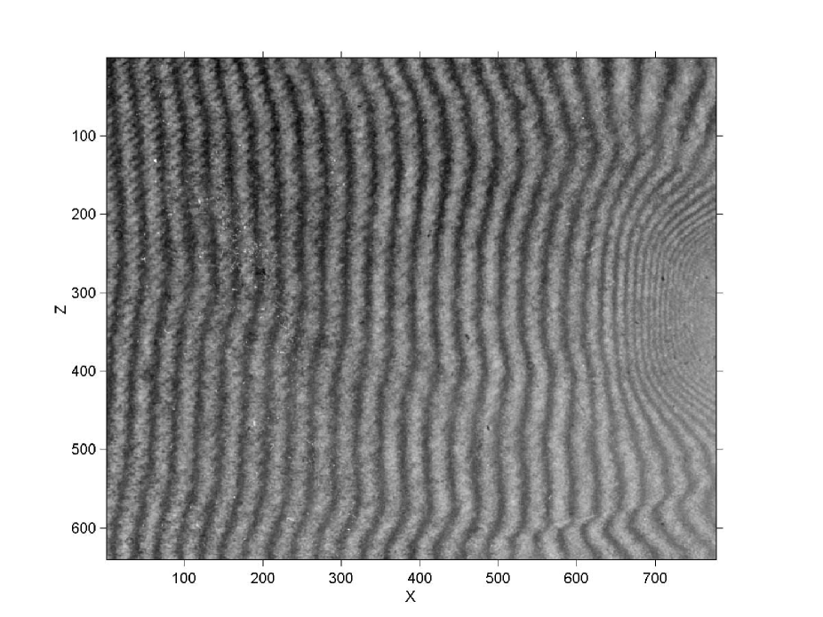
Figure 1:

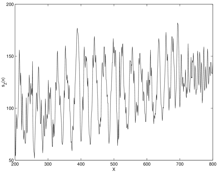
Figure 2:

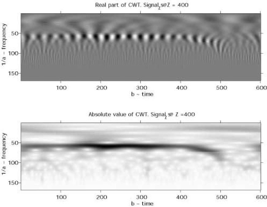
Figure 3:

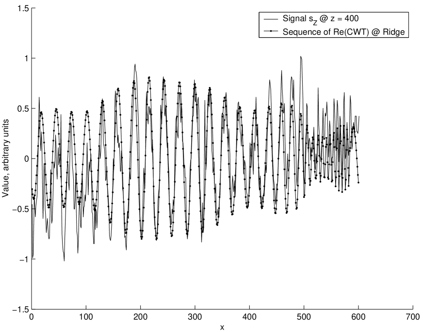
Figure 4:

Figure 5:

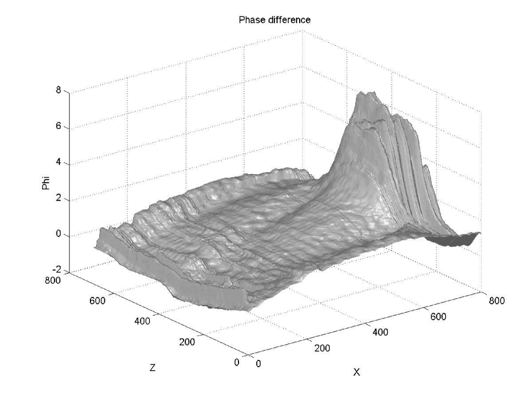
Figure 6:

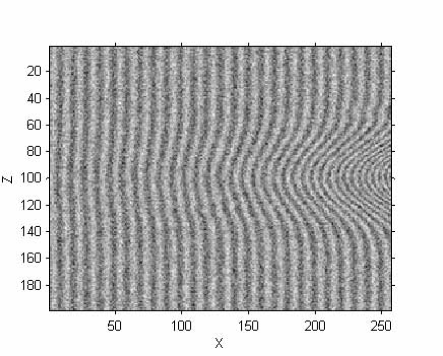
Figure 7:

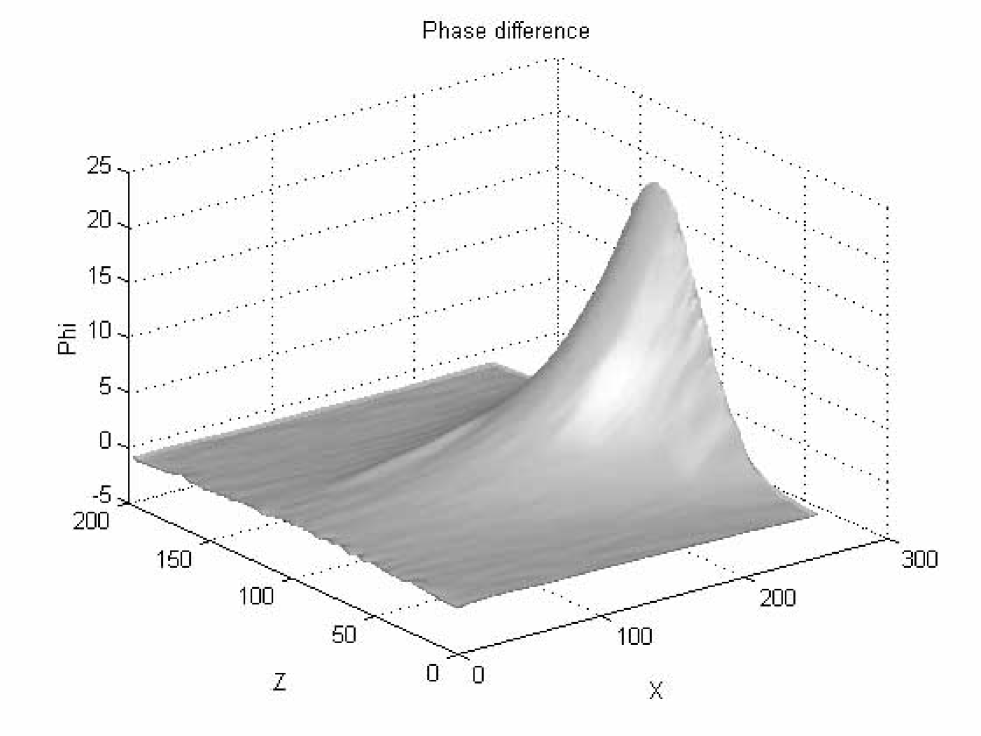
Figure 8:

.

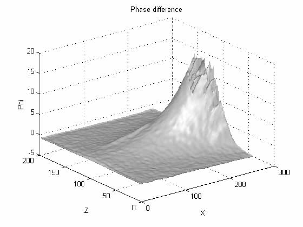
Figure 9:

.

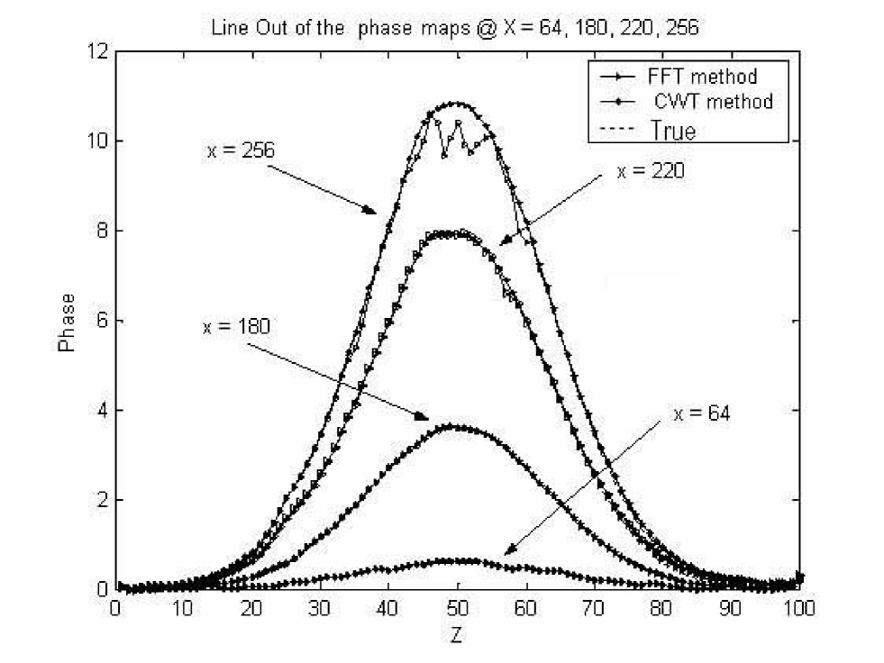
Figure 10:

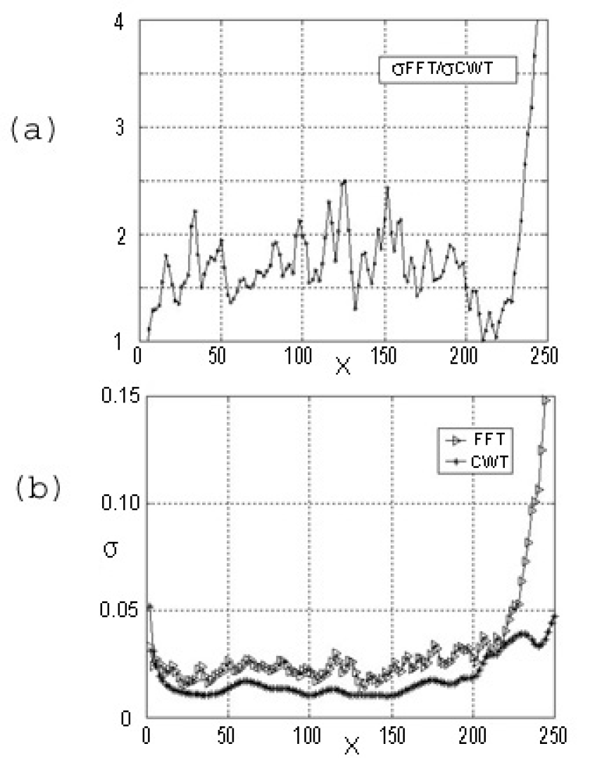
Figure 11:

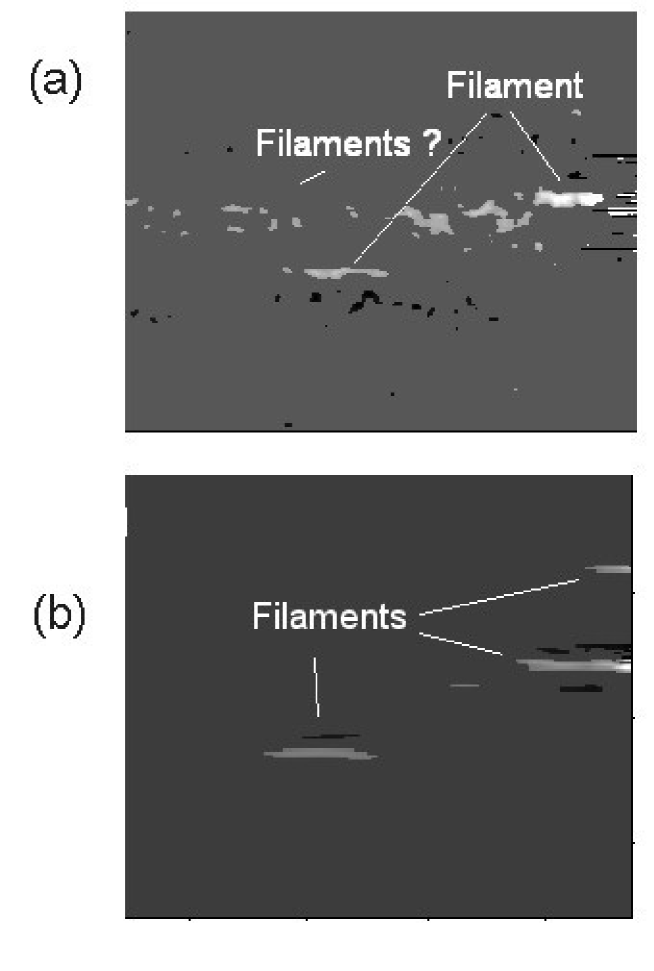
Figure 12:

References

- [1] R.Benattar, C.Popovics, R.Siegel, Polarized light interferometer for laser fusion studies, Rev.Sci.Instrum. 50, 1583 (1979)
- [2] O.Willi, Diagnostics and experimental methods of laser produced plasmas, in Laser-Plasma Interaction 4, Proceedings of XXXV Scottish Universities Summer School in Physics, St.Andrews, SUSSP Publications, University of Edinburg, 1988
- [3] P. Tomassini and A. Giulietti, A generalization of Abel Inversion to non axisymmetric density distribution, accepted for pub. on Opt. Comm.
- [4] M.Takeda, H.Ina, S.Kobayashi, Fourier-transform method of fringe-pattern analysis for computer-based topography and interferometry, J.Opt.Soc.Am. 72, 156 (1982).
- [5] K.A.Nugent, Interferogram analysis using an accurate fully automatic algorithm, Applied Optics 18, 3101 (1985)
- [6] L.A.Gizzi,D.Giulietti, A.Giulietti, T.Afshar-Rad, V.Biancalana, P.Chessa, E.Schifano, S.M.Viana, O.Willi, Characterisation of Laser Plasmas for Interaction Studies, Phys.Rev. E, 49, 5628 (1994)
- [7] L.A.Gizzi,D.Giulietti, A.Giulietti, T.Afshar-Rad, V.Biancalana, P.Chessa, E.Schifano, S.M.Viana, O.Willi, Characterisation of Laser Plasmas for Interaction Studies. Erratum, Phys.Rev. E, 50, 4266 (1994)
- [8] M.Borghesi, A.Giulietti, D.Giulietti, L.A.Gizzi, A.Macchi, O.Willi, Characterization of laser plasmas for interaction studies: progress in time-resolved density mapping, Phys.Rev. E, 54, 6768 (1996)
- [9] D. Gabor; Theory of Communication, J. Inst. Electr. Eng., London, 93 (III), pp 429-457
- [10] J. Morlet, G. Arens, I. Fourgeau and D. Giard; Wave propagation and sampling theory, Geophysics, 47, pp. 203-236
- [11] M. Holschneider; Wavelet: An analysis tool, Clarendon Press -Oxford (1995)
- [12] I. Daubechies; Ten lectures on Wavelets, Soc. for Ind. and Applied Mathematics, Philadelphia (1992)
- [13] R. Carmona, W.L. Hwang and B. Torresani; Characterization of Signals by the Ridges of their Wavelet Transform. paper; IEEE Trans. Signal Processing 45, vol. 10, p. 2586.
- [14] B. Torresani;Time Frequency and Time Scale Analysis, abstract in Signal Processing for Multimedia, J. Byrnes Ed. (1999) p. 37-52.
- [15] J.M. Innocent and B. Torresani; A Multiresolution Strategy for Detection Gravitational Waves Generated by Binary Coalescence, Submitted to Phys. Rev. D