Metastability in simple climate models:
Pathwise analysis of slowly driven Langevin equations

Abstract

We consider simple stochastic climate models, described by slowly time-dependent Langevin equations. We show that when the noise intensity is not too large, these systems can spend substantial amounts of time in metastable equilibrium, instead of adiabatically following the stationary distribution of the frozen system. This behaviour can be characterized by describing the location of typical paths, and bounding the probability of atypical paths. We illustrate this approach by giving a quantitative description of phenomena associated with bistability, for three famous examples of simple climate models: Stochastic resonance in an energy balance model describing Ice Ages; hysteresis in a box model for the Atlantic thermohaline circulation; and bifurcation delay in the case of the Lorenz model for Rayleigh–Bénard convection.

Date. November 4, 2001.

2000 Mathematical Subject Classification. 37H20 (primary), 60H10, 34E15, 82C31 (secondary).

Keywords and phrases. Stochastic resonance, dynamical hysteresis, bifurcation delay, double-well potential, first-exit time, scaling laws, Lorenz model, thermohaline circulation, white noise, coloured noise.

1 Introduction

One of the main difficulties of realistic climate models is that they involve a huge number of interacting degrees of freedom, on a wide range of time and length scales. In order to be able to control these models analytically, or at least numerically, it is necessary to simplify them by eliminating the less relevant degrees of freedom (e.g. high-frequency or short-wavelength modes). A possible way to do this is to average the equations of motion over all fast degrees of freedom, a rather drastic approximation. As proposed by Hasselmann [20] (see also [2]), a more realistic approximation is obtained by modeling the effect of fast degrees of freedom by noise.

In a number of cases, it is appropriate to distinguish between three rather than two time scales: Fast degrees of freedom (e.g. the “weather”), which are modeled by a stochastic process; intermediate “dominant modes” (e.g. the average temperature of the atmosphere) whose dynamics we want to predict; and slow degrees of freedom (e.g. the mean insolation depending on the eccentricity of the Earth’s orbit), which evolve on very long time scales of several centuries or millennia, and can be viewed as an external forcing. Such a system can often be modeled by a slowly time-dependent Langevin equation

$$\operatorname{d}\!x_{t}=f(x_{t},\varepsilon t)\operatorname{d}\!t+\sigma G(\varepsilon t)\operatorname{d}\!W_{t},$$ (1.1)

where the adiabatic parameter $\varepsilon$ and the noise intensity $\sigma$ are small parameters, $W_{t}$ is a standard vector-valued Wiener process (describing white noise) and $G$ is a matrix.

Our aim in this paper is to describe the effect of the noise term on the dynamics of (1.1), assuming the dynamics without noise is known. For this purpose, we will concentrate on bistable systems, which frequently occur in simple climate models: For instance, in models for the major Ice Ages, where the two possible stable equilibria correspond to warm and cold climate [4], or in models of the Atlantic thermohaline circulation [34, 30]. Noise may enable transitions between the two stable states, which would be impossible in the deterministic case, and our main concern will be to quantify this effect.

The method used to study the stochastic differential equation (SDE) (1.1) will depend on the time scale we are interested in. Let us first illustrate this on a static one-dimensional example, namely the overdamped motion in a symmetric double-well potential:

$$\operatorname{d}\!x_{t}=-\frac{\partial}{\partial x}V(x_{t})\operatorname{d}\!t+\sigma\operatorname{d}\!W_{t},\qquad V(x)=\frac{1}{4}bx^{4}-\frac{1}{2}ax^{2}.$$ (1.2)

where $a$ and $b$ are positive constants. The potential has two wells at $\pm\sqrt{a/b}$, separated by a barrier of height $H=a^{2}/(4b)$. A first possibility to analyse this equation is to compute the probability density $p(x,t)$ of $x_{t}$. It obeys the Fokker–Planck equation

$$\frac{\partial}{\partial t}p(x,t)=\frac{\partial}{\partial x}\biggl{[}\frac{\partial V}{\partial x}(x)p(x,t)\biggr{]}+\frac{\sigma^{2}}{2}\frac{\partial^{2}}{\partial x^{2}}p(x,t),$$ (1.3)

which admits in particular the stationary solution

$$p_{0}(x)=\frac{1}{N}\operatorname{e}^{-2V(x)/\sigma^{2}},$$ (1.4)

where $N$ is the normalization. At equilibrium, there is equal probability to find $x_{t}$ in either potential well, and for weak noise it is unlikely to observe $x_{t}$ anywhere else than in a neighbourhood of order $\sigma$ of one of the wells.

Assume now that the initial distribution $x_{0}$ is concentrated at the bottom $\sqrt{a/b}$ of the right-hand potential well. Then it may take quite a long time for the density to approach its asymptotic value (1.4). A possible way to investigate this problem relies on spectral theory. Denote the right-hand side of (1.3) as ${\mathcal{L}}p(x,t)$, where ${\mathcal{L}}$ is a linear differential operator. The stationary density (1.4) is an eigenfunction of ${\mathcal{L}}$ with eigenvalue $0$. We may assume that ${\mathcal{L}}$ has eigenvalues $\dots<\lambda_{k}<\dots<\lambda_{2}<\lambda_{1}<0$, c.f. [21, Section 6.7]. Decomposing $p(x,t)$ on a basis of eigenfunctions of ${\mathcal{L}}$, we see that $p$ approaches the stationary solution in a characteristic time of order $1/\lvert\lambda_{1}\rvert$.

There exists, however, a much more precise description of the process $x_{t}$ than by its probability density. Recall that for almost every realization $W_{t}(\omega)$ of the Brownian motion, the sample path $t\mapsto x_{t}(\omega)$ is continuous. Instead of computing the time needed for $p(x,t)$ to relax to $p_{0}(x)$, we can consider the random variable

$$\tau(\omega)=\inf\bigl{\{}t>0\colon x_{t}(\omega)<0\bigr{\}},$$ (1.5)

describing the first time at which the path $x_{t}$ crosses the saddle (one could as well consider the first time the bottom of the left-hand well is reached). The distribution of $\tau$ is asymptotically exponential, with expectation behaving in the weak-noise limit like Kramers’ time

$$T_{\mathchoice{\mbox{$\displaystyle\rm Kramers$}}{\mbox{$\textstyle\rm Kramers$}}{\mbox{$\scriptstyle\rm Kramers$}}{\mbox{$\scriptscriptstyle\rm Kramers$}}}=\operatorname{e}^{2H/\sigma^{2}}.$$ (1.6)

A mathematical theory allowing to estimate first-exit times for general $n$-dimensional systems (with a drift term not necessarily deriving from a potential) has been developed by Freidlin and Wentzell [18]. In specific situations, more precise results are available, for instance subexponential corrections to the asymptotic expression (1.6), see [3, 15]. Even the limiting behaviour of the distribution of the first-exit time from a neighbourhood of a unique stable equilibrium point has been obtained [14]. The first-exit time from a neighbourhood of a saddle has been considered by Kifer in the seminal paper [25].

If the noise intensity $\sigma$ is small (compared to the square root of the barrier height), then the time needed to overcome the potential barrier is extremely long, and the time required to relax to the stationary distribution $p_{0}(x)$ is even longer. In fact, on time scales shorter than Kramers’ time, solutions of (1.2) starting in one potential well will hardly feel the second potential well. As we will see in Section 2, $x_{t}$ is well approximated by an Ornstein–Uhlenbeck process, describing the overdamped motion of a particle in a potential of constant curvature $c=2a$. The Ornstein–Uhlenbeck process relaxes to a stationary Gaussian process with variance $\sigma^{2}/(2c)$ in a characteristic time

$$T_{\mathchoice{\mbox{$\displaystyle\rm relax$}}{\mbox{$\textstyle\rm relax$}}{\mbox{$\scriptstyle\rm relax$}}{\mbox{$\scriptscriptstyle\rm relax$}}}=\frac{1}{c}.$$ (1.7)

Thus for $0\mathrel{\leqsymb}t\ll T_{\mathchoice{\mbox{$\displaystyle\rm relax$}}{\mbox{$\textstyle\rm relax$}}{\mbox{$\scriptstyle\rm relax$}}{\mbox{$\scriptscriptstyle\rm relax$}}}$, the behaviour of $x_{t}$ is transient; for $T_{\mathchoice{\mbox{$\displaystyle\rm relax$}}{\mbox{$\textstyle\rm relax$}}{\mbox{$\scriptstyle\rm relax$}}{\mbox{$\scriptscriptstyle\rm relax$}}}\ll t\ll T_{\mathchoice{\mbox{$\displaystyle\rm Kramers$}}{\mbox{$\textstyle\rm Kramers$}}{\mbox{$\scriptstyle\rm Kramers$}}{\mbox{$\scriptscriptstyle\rm Kramers$}}}$, $x_{t}$ is close to a stationary Ornstein–Uhlenbeck process with variance $\sigma^{2}/(2c)$; and only for $t\gg T_{\mathchoice{\mbox{$\displaystyle\rm Kramers$}}{\mbox{$\textstyle\rm Kramers$}}{\mbox{$\scriptstyle\rm Kramers$}}{\mbox{$\scriptscriptstyle\rm Kramers$}}}$ will the distribution of $x_{t}$ approach the bimodal stationary solution (1.4). This phenomenon, where a process seems stationary for a long time before ultimately relaxing to a new (possibly stationary) state, is known as metastability. It is all the more remarkable in an asymmetric double-well potential: then a process starting at the bottom of the shallow well will first relax to a metastable distribution concentrated in the shallow well, which is radically different from the stationary distribution having most of its mass concentrated in the deeper well.

A different approach, based on the concept of random attractors (see [12, 31, 1]), gives complementary information on the long-time regime. In particular, in [13] it is proved that for arbitrarily weak noise, paths of (1.2) with different initial conditions but same realization of noise almost surely converge to a random point. The time needed for this convergence, however, diverges rapidly in the limit $\sigma\to 0$, because paths starting in different potential wells are unlikely to overcome the potential barrier and start approaching each other before Kramers’ time.

We now turn to situations in which the potential varies slowly in time. For simplicity, we will consider the family of Ginzburg–Landau potentials

$$V(x,\lambda,\mu)=\frac{1}{4}x^{4}-\frac{1}{2}\mu x^{2}-\lambda x,$$ (1.8)

and let either $\lambda$ or $\mu$ vary in time, with low speed $\varepsilon$. For instance, $\lambda$ or $\mu$ may depend periodically on time, with low frequency $2\pi\varepsilon$. The potential $V$ has two wells if $27\lambda^{2}<4\mu^{3}$ and one well if $27\lambda^{2}>4\mu^{3}$, and when $\lambda$ or $\mu$ are varied, the number of wells may change. Crossing one of the curves $27\lambda^{2}=4\mu^{3}$, $\mu>0$, corresponds to a saddle–node bifurcation, and crossing the point $\lambda=\mu=0$ corresponds to a pitchfork bifurcation.

The slow time-dependence introduces a new time scale $T_{\mathchoice{\mbox{$\displaystyle\rm forcing$}}{\mbox{$\textstyle\rm forcing$}}{\mbox{$\scriptstyle\rm forcing$}}{\mbox{$\scriptscriptstyle\rm forcing$}}}=1/\varepsilon$. Since curvature and barrier height are no longer constant, we replace the definitions (1.6) and (1.7) by

$$T_{\mathchoice{\mbox{$\displaystyle\rm Kramers$}}{\mbox{$\textstyle\rm Kramers$}}{\mbox{$\scriptstyle\rm Kramers$}}{\mbox{$\scriptscriptstyle\rm Kramers$}}}^{(\mathchoice{\mbox{$\displaystyle\rm max$}}{\mbox{$\textstyle\rm max$}}{\mbox{$\scriptstyle\rm max$}}{\mbox{$\scriptscriptstyle\rm max$}})}=\operatorname{e}^{2H_{\mathchoice{\mbox{$\displaystyle\rm max$}}{\mbox{$\textstyle\rm max$}}{\mbox{$\scriptstyle\rm max$}}{\mbox{$\scriptscriptstyle\rm max$}}}/\sigma^{2}}\qquad\qquad\text{and}\qquad\qquad T_{\mathchoice{\mbox{$\displaystyle\rm relax$}}{\mbox{$\textstyle\rm relax$}}{\mbox{$\scriptstyle\rm relax$}}{\mbox{$\scriptscriptstyle\rm relax$}}}^{(\mathchoice{\mbox{$\displaystyle\rm min$}}{\mbox{$\textstyle\rm min$}}{\mbox{$\scriptstyle\rm min$}}{\mbox{$\scriptscriptstyle\rm min$}})}=\frac{1}{c_{\mathchoice{\mbox{$\displaystyle\rm max$}}{\mbox{$\textstyle\rm max$}}{\mbox{$\scriptstyle\rm max$}}{\mbox{$\scriptscriptstyle\rm max$}}}},$$ (1.9)

where $H_{\mathchoice{\mbox{$\displaystyle\rm max$}}{\mbox{$\textstyle\rm max$}}{\mbox{$\scriptstyle\rm max$}}{\mbox{$\scriptscriptstyle\rm max$}}}$ denotes the maximal barrier height during one period, and $c_{\mathchoice{\mbox{$\displaystyle\rm max$}}{\mbox{$\textstyle\rm max$}}{\mbox{$\scriptstyle\rm max$}}{\mbox{$\scriptscriptstyle\rm max$}}}$ denotes the maximal curvature at the bottom of a potential well. Here we are interested in the regime

$$T_{\mathchoice{\mbox{$\displaystyle\rm relax$}}{\mbox{$\textstyle\rm relax$}}{\mbox{$\scriptstyle\rm relax$}}{\mbox{$\scriptscriptstyle\rm relax$}}}^{(\mathchoice{\mbox{$\displaystyle\rm min$}}{\mbox{$\textstyle\rm min$}}{\mbox{$\scriptstyle\rm min$}}{\mbox{$\scriptscriptstyle\rm min$}})}\ll T_{\mathchoice{\mbox{$\displaystyle\rm forcing$}}{\mbox{$\textstyle\rm forcing$}}{\mbox{$\scriptstyle\rm forcing$}}{\mbox{$\scriptscriptstyle\rm forcing$}}}\ll T_{\mathchoice{\mbox{$\displaystyle\rm Kramers$}}{\mbox{$\textstyle\rm Kramers$}}{\mbox{$\scriptstyle\rm Kramers$}}{\mbox{$\scriptscriptstyle\rm Kramers$}}}^{(\mathchoice{\mbox{$\displaystyle\rm max$}}{\mbox{$\textstyle\rm max$}}{\mbox{$\scriptstyle\rm max$}}{\mbox{$\scriptscriptstyle\rm max$}})},$$ (1.10)

which means that the process has time to reach a metastable “equilibrium” during one period, but not the bimodal stationary distribution. Mathematically, we thus assume that $\varepsilon\ll c_{\mathchoice{\mbox{$\displaystyle\rm max$}}{\mbox{$\textstyle\rm max$}}{\mbox{$\scriptstyle\rm max$}}{\mbox{$\scriptscriptstyle\rm max$}}}$ and $\sigma^{2}\ll 2H_{\mathchoice{\mbox{$\displaystyle\rm max$}}{\mbox{$\textstyle\rm max$}}{\mbox{$\scriptstyle\rm max$}}{\mbox{$\scriptscriptstyle\rm max$}}}/\lvert\log\varepsilon\rvert$. We allow, however, the minimal curvature and barrier height to become small, or even to vanish.

For time-dependent potentials, the Fokker–Planck equation (1.3) is even harder to solve (and in fact, it does not admit a stationary solution). Moreover, random attractors are not straightforward to define in this time-dependent setting. We believe that the dynamics on time scales shorter than $\smash{T_{\mathchoice{\mbox{$\displaystyle\rm Kramers$}}{\mbox{$\textstyle\rm Kramers$}}{\mbox{$\scriptstyle\rm Kramers$}}{\mbox{$\scriptscriptstyle\rm Kramers$}}}^{(\mathchoice{\mbox{$\displaystyle\rm max$}}{\mbox{$\textstyle\rm max$}}{\mbox{$\scriptstyle\rm max$}}{\mbox{$\scriptscriptstyle\rm max$}})}}$ is discussed best via an understanding of “typical” paths. The idea is to show that the vast majority of paths remain concentrated in small space–time sets, whose shape and size depend on the potential and the noise intensity. These sets are typically located in a neighbourhood of the potential wells, but under some conditions paths may also switch potential wells. There are thus two problems to solve: first characterize the sets in which typical paths live, and then estimate the probability of atypical paths. It turns out that these properties have universal characteristics, depending only on qualitative properties of the potential, especially its bifurcation points.

We start, in Section 2, by discussing the simplest situation, which occurs when the initial condition of the process lies in the basin of attraction of a stable equilibrium branch. For sufficiently small noise intensity, the majority of paths remain concentrated for a long time in a neighbourhood of the equilibrium branch. We determine the shape of this neighbourhood and outline how coloured noise can decrease the spreading of paths.

Section 3 is devoted to the phenomenon of stochastic resonance. We first recall the energy-budget model introduced in [4] to give a possible explanation for the close-to-periodic appearance of the major Ice Ages. This model is equivalent to the overdamped motion of a particle in a modulated double-well potential, where the driving amplitude is too small to allow for transitions between wells in the absence of noise. Turning to the description of typical paths, we find a threshold value for the noise intensity below which the paths remain in one well, while above threshold, they switch back and forth between wells twice per period. The switching events occur close to the instants of minimal barrier height. Several important quantities have a power-law dependence on the small parameters, in particular the critical noise intensity, the width of transition windows, and the exponent controlling the exponential decay of the probability of atypical paths.

In Section 4, we start by discussing a variant [11] of Stommel’s box model [34] of the Atlantic thermohaline circulation. Assuming slow changes in the typical weather, this model also reduces to the motion in a modulated double-well potential, where the modulation depends on the freshwater flux. If the amplitude of the modulation exceeds a threshold, the potential barrier vanishes twice per period, so that the deterministic motion displays hysteresis. Additive noise influences the shape of hysteresis cycles, and may even create macroscopic cycles for subthreshold modulation amplitude. We characterize the distribution of the random freshwater flux causing the system to switch from one stable state to the other one.

Finally, in Section 5, we consider the Lorenz model for Rayleigh–Bénard convection with slowly increasing heating. In the deterministic case, convection rolls appear only some time after the steady state looses stability in a pitchfork bifurcation. This bifurcation delay is significantly decreased by additive noise, as soon as its intensity is not exponentially small.

2 Near stable equilibria

Let us start by investigating Equation (1.1) in the one-dimensional case, i.e., when $x_{t}$, $W_{t}$ and $G(t)=g(t)$ are scalar. Since we are interested in the dynamics on the time scale $T_{\mathchoice{\mbox{$\displaystyle\rm forcing$}}{\mbox{$\textstyle\rm forcing$}}{\mbox{$\scriptstyle\rm forcing$}}{\mbox{$\scriptscriptstyle\rm forcing$}}}=1/\varepsilon$, we rescale time by a factor $\varepsilon$, which results in the SDE

$$\operatorname{d}\!x_{t}=\frac{1}{\varepsilon}f(x_{t},t)\operatorname{d}\!t+\frac{\sigma}{\sqrt{\varepsilon}}g(t)\operatorname{d}\!W_{t}.$$ (2.1)

The factor $1/\sqrt{\varepsilon}$ is due to the diffusive nature of the Brownian motion.

In this section, we will consider the dynamics near a stable equilibrium branch of $f$, i.e., a curve $x^{\star}(t)$ such that

$$f(x^{\star}(t),t)=0\qquad\text{and}\qquad a^{\star}(t)=\frac{\partial f}{\partial x}(x^{\star}(t),t)\mathrel{\leqsymb}-a_{0}$$ (2.2)

for all $t$, where $a_{0}$ is a positive constant. In the one-dimensional case, $f$ always derives from a potential $V$, and $-a^{\star}(t)$ represents the curvature at the bottom $x^{\star}(t)$ of a potential well.

In the deterministic case $\sigma=0$, solutions of (2.1) track the equilibrium branch $x^{\star}(t)$ adiabatically. In fact, Tihonov’s Theorem [36, 19] asserts that for $\sigma=0$, (2.1) admits a particular solution $\bar{x}^{\det}_{t}$ with an asymptotic expansion of the form

$$\bar{x}^{\det}_{t}=x^{\star}(t)+\varepsilon\frac{\dot{x}^{\star}(t)}{a^{\star}(t)}+{\mathcal{O}}(\varepsilon^{2}).$$ (2.3)

Since $a^{\star}(t)$ is negative, $\bar{x}^{\det}_{t}$ lies a little bit to the left of $x^{\star}(t)$ if $x^{\star}(t)$ moves to the right, and vice versa. The adiabatic solution $\bar{x}^{\det}_{t}$ attracts nearby solutions exponentially fast in $t/\varepsilon$.

Consider now the SDE (2.1) with positive noise intensity. For the sake of brevity, we assume that $g$ is positive and bounded away from zero. In a nutshell, our main result can be formulated as follows: Up to Kramer’s time, paths starting near $\bar{x}^{\det}_{0}$ are concentrated in a neighbourhood of order $\sigma g(t)/\sqrt{\lvert a^{\star}(t)\rvert}$ of the deterministic solution with the same initial condition, as shown in Figure 1. Larger noise intensities and smaller curvatures thus lead to a larger spreading of paths. This result holds as long as the spreading is smaller than the distance between $x^{\star}(t)$ and the nearest unstable equilibrium (i.e., the nearest saddle of the potential).

To make this claim mathematically precise, we need a few definitions. For simplicity, we discuss first the particular case $x_{0}=\bar{x}^{\det}_{0}$. We use the notations

$$a(t)=\frac{\partial f}{\partial x}(\bar{x}^{\det}_{t},t),\qquad\alpha(t,s)=\int_{s}^{t}a(u)\operatorname{d}\!u\qquad\text{and}\qquad\alpha(t)=\alpha(t,0).$$ (2.4)

Note that by (2.3), $a(t)=a^{\star}(t)+{\mathcal{O}}(\varepsilon)$ is negative for sufficiently small $\varepsilon$. The main idea is that $x_{t}-\bar{x}^{\det}_{t}$ is well approximated by a generalized Ornstein–Uhlenbeck process, with time-dependent damping $a(t)/\varepsilon$ and diffusion coefficient $\sigma g(t)/\sqrt{\varepsilon}$. This process is obtained by linearizing the SDE (2.1) around $\bar{x}^{\det}_{t}$, and has variance

$$v(t)=\frac{\sigma^{2}}{\varepsilon}\int_{0}^{t}\operatorname{e}^{2\alpha(t,s)/\varepsilon}g(s)^{2}\operatorname{d}\!s.$$ (2.5)

The function $v(t)$ solves the ordinary differential equation (ODE) $\varepsilon\dot{v}=2a(t)v+\sigma^{2}g(t)^{2}$. In analogy with (2.3), this equation also admits a particular solution $\bar{v}(t)$ satisfying

$$\bar{v}(t)=\frac{\sigma^{2}}{2\lvert a(t)\rvert}\bigl{[}g(t)^{2}+{\mathcal{O}}(\varepsilon)\bigr{]},$$ (2.6)

and since $\alpha(t)\mathrel{\leqsymb}-a_{0}t$ for $t\mathrel{\geqsymb}0$, the variance $v(t)=\bar{v}(t)-\bar{v}(0)\operatorname{e}^{2\alpha(t)/\varepsilon}$ approaches $\bar{v}(t)$ exponentially fast. We now introduce the set

$${\mathcal{B}}(h)=\bigl{\{}(x,t)\colon\lvert x-\bar{x}^{\det}_{t}\rvert<h\sqrt{\bar{v}(t)}\bigr{\}},$$ (2.7)

which depends on a real parameter $h>0$. The strip ${\mathcal{B}}(h)$ is centred in the adiabatic solution $\bar{x}^{\det}_{t}$ tracking the bottom of the potential well, and has time-dependent width $h\sigma g(t)/\sqrt{2\lvert a^{\star}(t)\rvert}[1+{\mathcal{O}}(\varepsilon)]$. To lowest order in $\varepsilon$ and $\sigma$, ${\mathcal{B}}(h)$ coincides with the points in the potential well for which $V(x,t)-V(\bar{x}^{\det}_{t},t)$ is smaller than $(\frac{1}{2}h\sigma g(t))^{2}$.

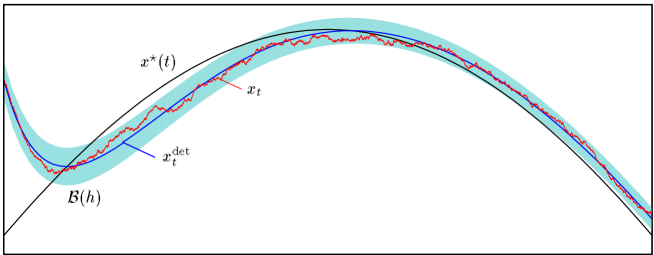
Figure 1: A sample path of the SDE (2.1), for $f(x,t)=a^{\star}(t)(x-x^{\star}(t))$ deriving from a quadratic single-well potential, and $g(t)\equiv 1$. The potential well is located at $x^{\star}(t)=\sin(2\pi t)$, and has curvature $-a^{\star}(t)=4-2\sin(4\pi t)$. Parameter values are $\varepsilon=0.04$ and $\sigma=0.025$. After a short transient motion, the deterministic solution $x^{\det}_{t}$ tracks $x^{\star}(t)$ at a distance of order $\varepsilon$. The path $x_{t}$ is likely to stay in the shaded set ${\mathcal{B}}(h)$ (shown here for $h=3$), which is centred at $x^{\det}_{t}$ and has time-dependent width of order $h\sigma/\sqrt{\lvert a^{\star}(t)\rvert}$.

The main result is that for $h\gg 1$, paths $\{x_{s}\}_{s\mathrel{\geqsymb}0}$ are unlikely to leave the set ${\mathcal{B}}(h)$ before Kramers’ time. Equivalently, the first-exit time

$$\tau_{{\mathcal{B}}(h)}=\inf\bigl{\{}t>0\colon(x_{t},t)\not\in{\mathcal{B}}(h)\bigr{\}}$$ (2.8)

is unlikely to be smaller than $T_{\mathchoice{\mbox{$\displaystyle\rm Kramers$}}{\mbox{$\textstyle\rm Kramers$}}{\mbox{$\scriptstyle\rm Kramers$}}{\mbox{$\scriptscriptstyle\rm Kramers$}}}$. Indeed, one can prove the following estimate (see [6, Theorem 2.4] and [8, Theorem 2.2]). There is a constant $h_{0}>0$ such that

$$\mathbb{P}\bigl{\{}\tau_{{\mathcal{B}}(h)}>t\bigr{\}}\mathrel{\leqsymb}C(t,\varepsilon)\operatorname{e}^{-\kappa h^{2}}$$ (2.9)

holds for all $t>0$ and all $h\mathrel{\leqsymb}h_{0}/\sigma$, where

$$C(t,\varepsilon)=\frac{\lvert\alpha(t)\rvert}{\varepsilon^{2}}+2\qquad\text{and}\qquad\kappa=\frac{1}{2}-{\mathcal{O}}(\varepsilon)-{\mathcal{O}}(\sigma h).$$ (2.10)

The exponential term $\operatorname{e}^{-\kappa h^{2}}$ in (2.9) is independent of time, and becomes small as soon as $h\gg 1$. The constant $h_{0}$ depends on $f$ and is the smaller the smaller $a_{0}$ is: The flatter the well, the more restrictive the condition $h\mathrel{\leqsymb}h_{0}/\sigma$ becomes. The prefactor $C(t,\varepsilon)$, which grows as time increases (and is certainly not optimal) only leads to subexponential corrections on the time scale $T_{\mathchoice{\mbox{$\displaystyle\rm forcing$}}{\mbox{$\textstyle\rm forcing$}}{\mbox{$\scriptstyle\rm forcing$}}{\mbox{$\scriptscriptstyle\rm forcing$}}}$. Some time dependence of the prefactor is to be expected, as it reflects the fact that occasionally a path will make an unusually large excursion, and the longer we wait the more excursions we will observe. The prefactor also depends on $\varepsilon$. A factor $1/\varepsilon$ is due to the fact that we are working on the time scale $T_{\mathchoice{\mbox{$\displaystyle\rm forcing$}}{\mbox{$\textstyle\rm forcing$}}{\mbox{$\scriptstyle\rm forcing$}}{\mbox{$\scriptscriptstyle\rm forcing$}}}$, while the actual factor of $1/\varepsilon^{2}$ allows us to obtain the best possible exponent. Choosing $\kappa$ slightly smaller allows to replace $\varepsilon^{2}$ by the more natural $\varepsilon$ in the definition of $C(t,\varepsilon)$. Thus we find that paths are unlikely to leave ${\mathcal{B}}(h)$ before time $t$, provided $h_{0}^{2}/\sigma^{2}\mathrel{\geqsymb}h^{2}\gg\log C(t,\varepsilon)$.

The same results hold if $x_{t}$ does not start on the adiabatic solution $\bar{x}^{\det}_{t}$, but in some deterministic $x_{0}$ sufficiently close to it. Then $\bar{x}^{\det}_{t}$ has to be replaced in (2.4) and (2.7) by the solution $x^{\det}_{t}$ of the deterministic equation with initial condition $x_{0}$. We still have that $a(t)$ is negative (and bounded away from zero), but note that (2.6) may not hold for very small $t$, when $x^{\det}_{t}$ has not yet approached $\bar{x}^{\det}_{t}$.

If the potential $V$ grows at least quadratically for large $\lvert x\rvert$, one can deduce from (2.9) that the moments of $\lvert x_{t}-x^{\det}_{t}\rvert$ are bounded by those of a centred Gaussian distribution with variance of order $\bar{v}(t)$, for times small compared to Kramers’ time [8, Corollary 2.4], even if $V$ has other potential wells than the one at $x^{\star}(t)$. Assume for instance that $V$ has two potential wells, with the shallower one at $x^{\star}(t)$. Then the system is in metastable “equilibrium” for an exponentially long time span during which the existence of the deeper well is not felt.

Similar statements are valid in the multidimensional case (in which $f$ does not necessarily derive from a potential). Let $x^{\star}(t)$ be an equilibrium branch of $f$, and denote by $A^{\star}(t)$ the Jacobian matrix of $f$ at $x^{\star}(t)$. We assume that the eigenvalues of $A^{\star}(t)$ have real parts smaller than some negative constant $-a_{0}$ for all times, so that $x^{\star}(t)$ is asymptotically stable. In the deterministic case $\sigma=0$, Tihonov’s theorem shows the existence of an adiabatic solution

$$\bar{x}^{\det}_{t}=x^{\star}(t)+\varepsilon A^{\star}(t)^{-1}\dot{x}^{\star}(t)+{\mathcal{O}}(\varepsilon^{2}),$$ (2.11)

which attracts nearby orbits exponentially fast. Let $A(t)$ be the Jacobian matrix of $f$ at $\bar{x}^{\det}_{t}$. It satisfies $A(t)=A^{\star}(t)+{\mathcal{O}}(\varepsilon)$. The solution of the SDE (1.1) linearized at $\bar{x}^{\det}_{t}$ has a Gaussian distribution, with covariance matrix

$$X(t)=\frac{\sigma^{2}}{\varepsilon}\int_{0}^{t}U(t,s)G(s)G(s)^{T}U(t,s)^{T}\operatorname{d}\!s,$$ (2.12)

where $U(t,s)$ is the fundamental solution of $\varepsilon\dot{y}=A(t)y$ with initial condition $U(s,s)={\mathchoice{\rm 1\mskip-4.0mul}{\rm 1\mskip-4.0mul}{\rm 1\mskip-4.5mul}{\rm 1\mskip-5.0mul}}$. To keep the presentation simple, we will assume that the smallest eigenvalue of $G(s)G(s)^{T}$ is bounded away from zero and the largest one is bounded above. Note that $X(t)$ obeys the ODE $\varepsilon\dot{X}=AX+XA^{T}+\sigma^{2}GG^{T}$, and approaches exponentially fast a matrix ${\mathchoice{{\hbox to0.0pt{\hbox to8.79166pt{$\hss\displaystyle{\overline{\hbox{}}}\mkern 0.5mu$}\hss}}}{{\hbox to0.0pt{\hbox to8.79166pt{$\hss\textstyle{\overline{\hbox{}}}\mkern 0.5mu$}\hss}}}{{\hbox to0.0pt{\hbox to6.07083pt{$\hss\scriptstyle{\overline{\hbox{}}}\mkern 0.5mu$}\hss}}}{{\hbox to0.0pt{\hbox to4.25694pt{$\hss\scriptscriptstyle{\overline{\hbox{}}}\mkern 0.5mu$}\hss}}}}X(t)$ which satisfies

$${\mathchoice{{\hbox to0.0pt{\hbox to8.79166pt{$\hss\displaystyle{\overline{\hbox{}}}\mkern 0.5mu$}\hss}}}{{\hbox to0.0pt{\hbox to8.79166pt{$\hss\textstyle{\overline{\hbox{}}}\mkern 0.5mu$}\hss}}}{{\hbox to0.0pt{\hbox to6.07083pt{$\hss\scriptstyle{\overline{\hbox{}}}\mkern 0.5mu$}\hss}}}{{\hbox to0.0pt{\hbox to4.25694pt{$\hss\scriptscriptstyle{\overline{\hbox{}}}\mkern 0.5mu$}\hss}}}}X(t)={\mathchoice{{\hbox to0.0pt{\hbox to8.79166pt{$\hss\displaystyle{\overline{\hbox{}}}\mkern 0.5mu$}\hss}}}{{\hbox to0.0pt{\hbox to8.79166pt{$\hss\textstyle{\overline{\hbox{}}}\mkern 0.5mu$}\hss}}}{{\hbox to0.0pt{\hbox to6.07083pt{$\hss\scriptstyle{\overline{\hbox{}}}\mkern 0.5mu$}\hss}}}{{\hbox to0.0pt{\hbox to4.25694pt{$\hss\scriptscriptstyle{\overline{\hbox{}}}\mkern 0.5mu$}\hss}}}}X_{0}(t)+{\mathcal{O}}(\varepsilon),\qquad\text{where }A{\mathchoice{{\hbox to0.0pt{\hbox to8.79166pt{$\hss\displaystyle{\overline{\hbox{}}}\mkern 0.5mu$}\hss}}}{{\hbox to0.0pt{\hbox to8.79166pt{$\hss\textstyle{\overline{\hbox{}}}\mkern 0.5mu$}\hss}}}{{\hbox to0.0pt{\hbox to6.07083pt{$\hss\scriptstyle{\overline{\hbox{}}}\mkern 0.5mu$}\hss}}}{{\hbox to0.0pt{\hbox to4.25694pt{$\hss\scriptscriptstyle{\overline{\hbox{}}}\mkern 0.5mu$}\hss}}}}X_{0}+{\mathchoice{{\hbox to0.0pt{\hbox to8.79166pt{$\hss\displaystyle{\overline{\hbox{}}}\mkern 0.5mu$}\hss}}}{{\hbox to0.0pt{\hbox to8.79166pt{$\hss\textstyle{\overline{\hbox{}}}\mkern 0.5mu$}\hss}}}{{\hbox to0.0pt{\hbox to6.07083pt{$\hss\scriptstyle{\overline{\hbox{}}}\mkern 0.5mu$}\hss}}}{{\hbox to0.0pt{\hbox to4.25694pt{$\hss\scriptscriptstyle{\overline{\hbox{}}}\mkern 0.5mu$}\hss}}}}X_{0}A^{T}=-\sigma^{2}GG^{T}.$$ (2.13)

Given a deterministic solution $x^{\det}_{t}$, the definition of the set ${\mathcal{B}}(h)$ reads now

$${\mathcal{B}}(h)=\bigl{\{}(x,t)\colon(x-x^{\det}_{t})^{T}{\mathchoice{{\hbox to0.0pt{\hbox to8.79166pt{$\hss\displaystyle{\overline{\hbox{}}}\mkern 0.5mu$}\hss}}}{{\hbox to0.0pt{\hbox to8.79166pt{$\hss\textstyle{\overline{\hbox{}}}\mkern 0.5mu$}\hss}}}{{\hbox to0.0pt{\hbox to6.07083pt{$\hss\scriptstyle{\overline{\hbox{}}}\mkern 0.5mu$}\hss}}}{{\hbox to0.0pt{\hbox to4.25694pt{$\hss\scriptscriptstyle{\overline{\hbox{}}}\mkern 0.5mu$}\hss}}}}X(t)^{-1}(x-x^{\det}_{t})<h^{2}\bigr{\}},$$ (2.14)

and (2.9) generalizes to the following statement (see [8, Theorem 6.1] for a discussion; the proof will be given in [5]): There is a constant $h_{0}>0$ such that for all $h\mathrel{\leqsymb}h_{0}/\sigma$ and all $\kappa\in(0,1/2)$,

$$\mathbb{P}\bigl{\{}\tau_{{\mathcal{B}}(h)}>t\bigr{\}}\mathrel{\leqsymb}C(t,\varepsilon)\operatorname{e}^{-\kappa h^{2}(1-{\mathcal{O}}(\varepsilon)-{\mathcal{O}}(\sigma h))},$$ (2.15)

where

$$C(t,\varepsilon)=\Bigl{(}\frac{t}{\varepsilon^{2}}+1\Bigr{)}\Bigl{(}\frac{1}{1-2\kappa}\Bigr{)}^{n/2},$$ (2.16)

$n$ being the dimension of $x$. Paths are thus concentrated, up to a given time $t$, in sets of the form ${\mathcal{B}}(h)$, which have an ellipsoïdal cross-section defined by ${\mathchoice{{\hbox to0.0pt{\hbox to8.79166pt{$\hss\displaystyle{\overline{\hbox{}}}\mkern 0.5mu$}\hss}}}{{\hbox to0.0pt{\hbox to8.79166pt{$\hss\textstyle{\overline{\hbox{}}}\mkern 0.5mu$}\hss}}}{{\hbox to0.0pt{\hbox to6.07083pt{$\hss\scriptstyle{\overline{\hbox{}}}\mkern 0.5mu$}\hss}}}{{\hbox to0.0pt{\hbox to4.25694pt{$\hss\scriptscriptstyle{\overline{\hbox{}}}\mkern 0.5mu$}\hss}}}}X(t)$. Again the parameter $h$ must satisfy $h_{0}^{2}/\sigma^{2}\mathrel{\geqsymb}h^{2}\gg\log C(t,\varepsilon)$.

This result can be used, in particular, to understand the effect of coloured noise. Assume for instance that the one-dimensional system

$$\operatorname{d}\!x_{t}=f(x_{t},\varepsilon t)\operatorname{d}\!t+g(\varepsilon t)\operatorname{d}\!Z_{t}$$ (2.17)

is not driven by white noise, but by an Ornstein–Uhlenbeck process $Z_{t}$ obeying the SDE

$$\operatorname{d}\!Z_{t}=-\gamma Z_{t}\operatorname{d}\!t+\sigma\operatorname{d}\!W_{t}.$$ (2.18)

The equations (2.17) and (2.18) can be rewritten, on the time scale $1/\varepsilon$, as a two-dimensional system of the form (1.1) for $(x_{t},Z_{t})$. We assume that $f$ has a stable equilibrium branch $x^{\star}(t)$ with linearization $a^{\star}(t)\mathrel{\leqsymb}-a_{0}<0$. To leading order in $\varepsilon$, the asymptotic covariance matrix (2.13) is given by

$${\mathchoice{{\hbox to0.0pt{\hbox to8.79166pt{$\hss\displaystyle{\overline{\hbox{}}}\mkern 0.5mu$}\hss}}}{{\hbox to0.0pt{\hbox to8.79166pt{$\hss\textstyle{\overline{\hbox{}}}\mkern 0.5mu$}\hss}}}{{\hbox to0.0pt{\hbox to6.07083pt{$\hss\scriptstyle{\overline{\hbox{}}}\mkern 0.5mu$}\hss}}}{{\hbox to0.0pt{\hbox to4.25694pt{$\hss\scriptscriptstyle{\overline{\hbox{}}}\mkern 0.5mu$}\hss}}}}X_{0}(t)=\sigma^{2}\begin{pmatrix}\vrule height=11.0pt,depth=16.0pt,width=0.0pt\dfrac{g(t)^{2}}{2(\gamma+\lvert a^{\star}(t)\rvert)}&\dfrac{g(t)}{2(\gamma+\lvert a^{\star}(t)\rvert)}\\ \vrule height=16.0pt,depth=11.0pt,width=0.0pt\dfrac{g(t)}{2(\gamma+\lvert a^{\star}(t)\rvert)}&\dfrac{1}{2\gamma}\end{pmatrix}.$$ (2.19)

The conditions on $GG^{T}$ mentioned above can be relaxed (c.f. [8, Theorem 6.1]), so that (2.15) is applicable. We find in particular that the path $\{x_{t}\}_{t\mathrel{\geqsymb}0}$ is concentrated in a strip of width proportional to $\sigma g(t)/\sqrt{\gamma+\lvert a^{\star}(t)\rvert}$, centred around $x^{\det}_{t}$. Hence larger “noise colour” $\gamma$ yields a smaller spreading of the paths, in the same way as if the curvature of the potential were increased by $\gamma$.

3 Stochastic resonance

In the previous section, we have seen that on a certain time scale, paths typically remain in metastable equilibrium. With overwhelming probability, they are concentrated in a strip of order $\sigma g(t)/\sqrt{\lvert a^{\star}(t)\rvert}$ near the bottom of a potential well with curvature $\lvert a^{\star}(t)\rvert$. This roughly holds as long as the strip does not extend to the nearest saddle of the potential. New phenomena may occur when this hypothesis is violated, either because the noise coefficient $\sigma g(t)$ becomes too large, or because the curvature or the distance to the saddle become too small. Then paths may overcome the potential barrier and reach another potential well. This mechanism has various interesting consequences, one of them being the effect called stochastic resonance.

Stochastic resonance (SR) was initially introduced as a possible explanation for the close-to-periodic appearance of the major Ice Ages [4]. While this explanation remains controversial, SR has been detected in several other physical and biological systems, see for instance [29, 39] for a review.

The original model in [4] is based on an energy balance of the Earth in integrated form. The evolution of the mean surface temperature $T$ is described by the differential equation

$$c\frac{\operatorname{d}\!T}{\operatorname{d}\!t}=Q(1+A\cos\omega t)(1-\alpha(T))-E(T).$$ (3.1)

Here the term $R_{\mathchoice{\mbox{$\displaystyle\rm in$}}{\mbox{$\textstyle\rm in$}}{\mbox{$\scriptstyle\rm in$}}{\mbox{$\scriptscriptstyle\rm in$}}}=Q(1+A\cos\omega t)$ is the incoming solar radiation, where $Q$ denotes the solar constant, and the periodic term models the effect of the Earth’s varying orbital eccentricity. The amplitude $A$ of this modulation is very small, of the order $5\times 10^{-4}$, while its period $2\pi/\omega$ equals $92\mskip 3.0mu000$ years. The outgoing radiation $R_{\mathchoice{\mbox{$\displaystyle\rm out$}}{\mbox{$\textstyle\rm out$}}{\mbox{$\scriptstyle\rm out$}}{\mbox{$\scriptscriptstyle\rm out$}}}=\alpha(T)R_{\mathchoice{\mbox{$\displaystyle\rm in$}}{\mbox{$\textstyle\rm in$}}{\mbox{$\scriptstyle\rm in$}}{\mbox{$\scriptscriptstyle\rm in$}}}+E(T)$ depends on the albedo $\alpha(T)$ of the Earth and its emissivity. $c$ denotes the heat capacity.

To account for the existence of two stable climate states (warm climate and Ice Age), the right-hand side of (3.1) should have two stable and one unstable equilibrium points. The authors of [4] postulate that

$$\gamma(T)=\frac{Q}{E(T)}(1-\alpha(T))-1=\beta\biggl{(}1-\frac{T}{T_{1}}\biggr{)}\biggl{(}1-\frac{T}{T_{2}}\biggr{)}\biggl{(}1-\frac{T}{T_{3}}\biggr{)},$$ (3.2)

where $T_{1}=278.6$ K and $T_{3}=288.6$ K are the representative temperatures of the two stable states, and $T_{2}=283.3$ K represents the unstable state. Since $E(T)\sim T^{4}$ varies little on this range, the problem can be further simplified by neglecting the $T$-dependence of $E(T)\simeq\langle E\rangle$. Equation (3.1) becomes

$$\frac{\operatorname{d}\!T}{\operatorname{d}\!t}=\frac{\langle E\rangle}{c}\biggl{[}\beta\biggl{(}1-\frac{T}{T_{1}}\biggr{)}\biggl{(}1-\frac{T}{T_{2}}\biggr{)}\biggl{(}1-\frac{T}{T_{3}}\biggr{)}(1+A\cos\omega t)+A\cos\omega t\biggr{]}.$$ (3.3)

The parameter $\beta$ is related to the relaxation time $\tau\simeq 8$ years of the system via

$$\frac{1}{\tau}=\frac{\langle E\rangle}{c}\beta\frac{1}{T_{3}}\biggl{(}1-\frac{T_{3}}{T_{1}}\biggr{)}\biggl{(}1-\frac{T_{3}}{T_{2}}\biggr{)}.$$ (3.4)

Let us now transform this system to a dimensionless form. We do this in two steps: First we scale time by a factor $\omega/2\pi$, so that in the new variables, the system has period $1$. Then we introduce the variable $x=(T-T_{2})/\Delta T$, where $\Delta T=(T_{3}-T_{1})/2=5$ K. The resulting system is

$$\frac{\operatorname{d}\!x}{\operatorname{d}\!t}=\frac{1}{\varepsilon}\bigl{[}-x(x-x_{1})(x-x_{3})(1+A\cos 2\pi t)+K\cos 2\pi t\bigr{]},$$ (3.5)

where $x_{1}=(T_{1}-T_{2})/\Delta T\simeq-0.94$ and $x_{3}=(T_{3}-T_{2})/\Delta T\simeq 1.06$. The adiabatic parameter $\varepsilon$ is given by

$$\varepsilon=\frac{\omega\tau}{2\pi}\mskip 3.0mu\frac{2(T_{3}-T_{2})}{\Delta T}\simeq 1.8\times 10^{-4}.$$ (3.6)

This confirms that we are in the adiabatic regime. Using the value $\langle E\rangle/c=8.77\times 10^{-3}/4000$ $\text{Ks}^{-1}$ from [4], we find a driving amplitude

$$K=\frac{A}{\beta}\frac{T_{1}T_{2}T_{3}}{(\Delta T)^{3}}\simeq 0.12.$$ (3.7)

The term in brackets in (3.5) derives from a double-well potential, which is almost of the Ginzburg–Landau type (1.8). If we set, for simplicity, $x_{1}=-1$ and $x_{3}=1$, and neglect the term $A\cos 2\pi t$, then we obtain indeed a force deriving from the potential (1.8), with $\mu=1$ and $\lambda=K\cos 2\pi t$. This potential has two wells if and only if $\lvert\lambda\rvert<\lambda_{\mathchoice{\mbox{$\displaystyle\rm c$}}{\mbox{$\textstyle\rm c$}}{\mbox{$\scriptstyle\rm c$}}{\mbox{$\scriptscriptstyle\rm c$}}}=2/3\sqrt{3}\simeq 0.38$, and thus the amplitude $K$ of the forcing is too small to enable transitions between the potential wells. Note, however, that although $A$ is very small, $K$ is not negligible compared to $\lambda_{\mathchoice{\mbox{$\displaystyle\rm c$}}{\mbox{$\textstyle\rm c$}}{\mbox{$\scriptstyle\rm c$}}{\mbox{$\scriptscriptstyle\rm c$}}}$.

The main new idea in [4] is that if one models the effect of the “weather” by an additive noise term, then transitions between potential wells not only become possible but, due to the periodic forcing, these transitions will be more likely at some times than at others, so that the evolution of $T$ can be close to periodic. We will illustrate this on the model SDE

$$\operatorname{d}\!x_{t}=\frac{1}{\varepsilon}\bigl{[}x_{t}-x_{t}^{3}+K\cos 2\pi t\bigr{]}\operatorname{d}\!t+\frac{\sigma}{\sqrt{\varepsilon}}\operatorname{d}\!W_{t}.$$ (3.8)

However, the results in [7] apply to a more general class of periodically forced double-well potentials, including (3.5).

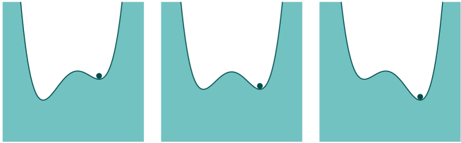
Figure 2: The potential $V(x,t)=\frac{1}{4}x^{4}-\frac{1}{2}x^{2}-K\cos(2\pi t)x$, from which derives the drift term in (3.8). For $\cos(2\pi t)=0$, the potential is symmetric (middle), for integer times, the left-hand well approaches the saddle (right), while for half-integer times, the right-hand well approaches the saddle (left). If the amplitude $K$ is smaller than the threshold $\lambda_{\mathchoice{\mbox{$\displaystyle\rm c$}}{\mbox{$\textstyle\rm c$}}{\mbox{$\scriptstyle\rm c$}}{\mbox{$\scriptscriptstyle\rm c$}}}$, there is always a potential barrier, which an overdamped particle cannot overcome in the deterministic case. Sufficiently strong noise, however, helps the particle to switch from the shallower to the deeper well. This effect is the stronger the lower the barrier is, so that switching typically occurs close to the instants of minimal barrier height.

Various characterizations of the effect of noise on the dynamics of (3.8), and various measures of periodicity have been proposed. A widespread approach uses the signal-to-noise ratio, a property of the power spectrum of $x_{t}$, which shows peaks near multiples of the driving frequency [16, 27, 24]. For small driving amplitudes $K$, the signal-to-noise ratio behaves like $\operatorname{e}^{-H/\sigma^{2}}/\sigma^{4}$, where $H$ is the height of the potential barrier in the absence of periodic driving (i.e., for $K=0$). The signal’s “periodicity” is thus optimal for $\sigma^{2}=H/2$. A different approach is used in [17], where the $L^{p}$-distance between sample paths and a periodic limiting function is shown to converge to zero in probability as $\sigma\to 0$. This result requires $\varepsilon$ to be of order $\operatorname{e}^{-2H/\sigma^{2}}$, which implies exponentially long forcing periods.

We examine here a different regime, in which the forcing amplitude $K$ is not necessarily a small parameter, but may approach $\lambda_{\mathchoice{\mbox{$\displaystyle\rm c$}}{\mbox{$\textstyle\rm c$}}{\mbox{$\scriptstyle\rm c$}}{\mbox{$\scriptscriptstyle\rm c$}}}$. In this way, transitions become possible for values of $\varepsilon$ which are not exponentially small. The potential barrier is lowest at integer and half-integer times. At integer times, the left-hand well approaches the saddle, while at half-integer times, the right-hand well approaches the saddle, c.f. Figure 2.

The minimal values $H_{\mathchoice{\mbox{$\displaystyle\rm min$}}{\mbox{$\textstyle\rm min$}}{\mbox{$\scriptstyle\rm min$}}{\mbox{$\scriptscriptstyle\rm min$}}}$, $c_{\mathchoice{\mbox{$\displaystyle\rm min$}}{\mbox{$\textstyle\rm min$}}{\mbox{$\scriptstyle\rm min$}}{\mbox{$\scriptscriptstyle\rm min$}}}$ and $\delta_{\mathchoice{\mbox{$\displaystyle\rm min$}}{\mbox{$\textstyle\rm min$}}{\mbox{$\scriptstyle\rm min$}}{\mbox{$\scriptscriptstyle\rm min$}}}$ of the barrier height, the curvature at the bottom of the wells, and the distance between the bottom of one of the wells and the saddle can be expressed as functions of a parameter $a_{0}=\lambda_{\mathchoice{\mbox{$\displaystyle\rm c$}}{\mbox{$\textstyle\rm c$}}{\mbox{$\scriptstyle\rm c$}}{\mbox{$\scriptscriptstyle\rm c$}}}-K$. For small $a_{0}$, they behave like $H_{\mathchoice{\mbox{$\displaystyle\rm min$}}{\mbox{$\textstyle\rm min$}}{\mbox{$\scriptstyle\rm min$}}{\mbox{$\scriptscriptstyle\rm min$}}}(a_{0})\asymp\smash{a_{0}^{3/2}}$, $c_{\mathchoice{\mbox{$\displaystyle\rm min$}}{\mbox{$\textstyle\rm min$}}{\mbox{$\scriptstyle\rm min$}}{\mbox{$\scriptscriptstyle\rm min$}}}(a_{0})\asymp\smash{a_{0}^{1/2}}$ and $\delta_{\mathchoice{\mbox{$\displaystyle\rm min$}}{\mbox{$\textstyle\rm min$}}{\mbox{$\scriptstyle\rm min$}}{\mbox{$\scriptscriptstyle\rm min$}}}(a_{0})\asymp\smash{a_{0}^{1/2}}$ (meaning $c_{-}\smash{a_{0}^{3/2}}\mathrel{\leqsymb}H_{\mathchoice{\mbox{$\displaystyle\rm min$}}{\mbox{$\textstyle\rm min$}}{\mbox{$\scriptstyle\rm min$}}{\mbox{$\scriptscriptstyle\rm min$}}}(a_{0})\mathrel{\leqsymb}c_{+}\smash{a_{0}^{3/2}}$ for some positive constants $c_{\pm}$ independent of $a_{0}$, and so on).

Intuitively, our results from Section 2 indicate that the maximal spreading of paths is of order $\sigma/\smash{c_{\mathchoice{\mbox{$\displaystyle\rm min$}}{\mbox{$\textstyle\rm min$}}{\mbox{$\scriptstyle\rm min$}}{\mbox{$\scriptscriptstyle\rm min$}}}(a_{0})^{1/2}}$, provided this value is smaller than $\delta_{\mathchoice{\mbox{$\displaystyle\rm min$}}{\mbox{$\textstyle\rm min$}}{\mbox{$\scriptstyle\rm min$}}{\mbox{$\scriptscriptstyle\rm min$}}}(a_{0})$, i.e., provided $\sigma\ll\smash{a_{0}^{3/4}}$. Assume for instance that we start at time $1/4$ (when the potential is symmetric) near the right-hand potential well. We call transition probability the probability $P_{\mathchoice{\mbox{$\displaystyle\rm trans$}}{\mbox{$\textstyle\rm trans$}}{\mbox{$\scriptstyle\rm trans$}}{\mbox{$\scriptscriptstyle\rm trans$}}}$ of having reached the left-hand potential well by time $3/4$, after passing through the configuration with the shallowest right-hand well. Extrapolating (2.9) with $h$ of the order $\delta_{\mathchoice{\mbox{$\displaystyle\rm min$}}{\mbox{$\textstyle\rm min$}}{\mbox{$\scriptstyle\rm min$}}{\mbox{$\scriptscriptstyle\rm min$}}}c_{\mathchoice{\mbox{$\displaystyle\rm min$}}{\mbox{$\textstyle\rm min$}}{\mbox{$\scriptstyle\rm min$}}{\mbox{$\scriptscriptstyle\rm min$}}}^{1/2}/\sigma\asymp H_{\mathchoice{\mbox{$\displaystyle\rm min$}}{\mbox{$\textstyle\rm min$}}{\mbox{$\scriptstyle\rm min$}}{\mbox{$\scriptscriptstyle\rm min$}}}^{1/2}/\sigma$, we find

$$P_{\mathchoice{\mbox{$\displaystyle\rm trans$}}{\mbox{$\textstyle\rm trans$}}{\mbox{$\scriptstyle\rm trans$}}{\mbox{$\scriptscriptstyle\rm trans$}}}\mathrel{\leqsymb}\frac{\text{\it const}}{\varepsilon^{2}}\operatorname{e}^{-\text{\it const }a_{0}^{3/2}/\sigma^{2}}=\frac{\text{\it const}}{\varepsilon^{2}}\operatorname{e}^{-\text{\it const }H_{\mathchoice{\mbox{$\displaystyle\rm min$}}{\mbox{$\textstyle\rm min$}}{\mbox{$\scriptstyle\rm min$}}{\mbox{$\scriptscriptstyle\rm min$}}}/\sigma^{2}}\qquad\qquad\text{for $\sigma\mathrel{\leqsymb}a_{0}^{3/4}$.}$$ (3.9)

Note the similarity with Kramers’ time for the potential frozen at the moment of minimal barrier height.

A bound of this form can indeed be proved, but (3.9) turns out to be a little bit too pessimistic for very small $a_{0}$. This is a rather subtle dynamical effect, related to the behaviour of the deterministic system. Recall that the set ${\mathcal{B}}(h)$ in (2.7) is defined via the linearization at the adiabatic solution $\bar{x}^{\det}_{t}$, not at the bottom $x^{\star}(t)$ of the potential well. This distinction is irrelevant as long as the minimal curvature remains of order one, but not when it is a small parameter. In that case, the asymptotic expansion (2.3) does not necessarily converge. Using methods from singular perturbation theory [10], one can show that $\bar{x}^{\det}_{t}$ never approaches the saddle closer than a distance of order $\sqrt{\varepsilon}$, so that the curvature at $\bar{x}^{\det}_{t}$ never becomes smaller than a quantity of order $\sqrt{\varepsilon}$, even if $a_{0}<\varepsilon$. As a consequence, for $a_{0}<\varepsilon$, the system behaves as if there were an effective potential barrier of height $\varepsilon^{3/2}$.

In fact, one can prove the following bound (see [7, Theorem 2.6] and [8, Theorem 3.1]): There exist constants $C,\kappa>0$ such that

$$P_{\mathchoice{\mbox{$\displaystyle\rm trans$}}{\mbox{$\textstyle\rm trans$}}{\mbox{$\scriptstyle\rm trans$}}{\mbox{$\scriptscriptstyle\rm trans$}}}\mathrel{\leqsymb}\frac{C}{\varepsilon}\operatorname{e}^{-\kappa\sigma_{\mathchoice{\mbox{$\displaystyle\rm c$}}{\mbox{$\textstyle\rm c$}}{\mbox{$\scriptstyle\rm c$}}{\mbox{$\scriptscriptstyle\rm c$}}}^{2}/\sigma^{2}}\qquad\qquad\text{for $\sigma\mathrel{\leqsymb}\sigma_{\mathchoice{\mbox{$\displaystyle\rm c$}}{\mbox{$\textstyle\rm c$}}{\mbox{$\scriptstyle\rm c$}}{\mbox{$\scriptscriptstyle\rm c$}}}=(a_{0}\vee\varepsilon)^{3/4}$,}$$ (3.10)

where $a\vee b$ denotes the maximum of two real numbers $a$ and $b$. In addition, paths remain concentrated in a set ${\mathcal{B}}(h)$ of the form (2.7). Examining the behaviour of the integral (2.5), one can show that the width of ${\mathcal{B}}(h)$ behaves, near $t=1/2$, like $h\sigma/(\lvert t-1/2\rvert^{1/2}\vee\smash{\sigma_{\mathchoice{\mbox{$\displaystyle\rm c$}}{\mbox{$\textstyle\rm c$}}{\mbox{$\scriptstyle\rm c$}}{\mbox{$\scriptscriptstyle\rm c$}}}^{1/3}})$. The various exponents entering these relations do not depend on the details of the potential, but only on some qualitative properties of the “avoided bifurcation”, and can be deduced geometrically from a Newton polygon [10].

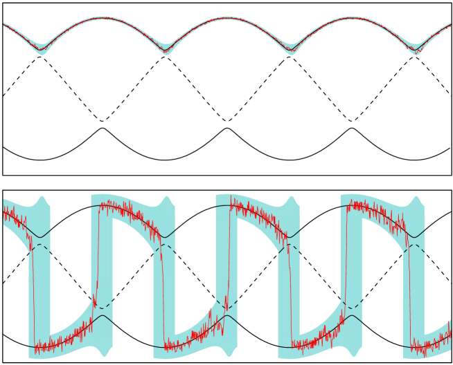
Figure 3: Sample paths of the SDE (3.8) for $\varepsilon=a_{0}=0.005$, and $\sigma=0.02$ (upper picture) and $\sigma=0.14$ (lower picture). Full curves represent the location of potential wells, the broken curve represents the saddle. For weak noise, the path $x_{t}$ is likely to stay in the shaded set ${\mathcal{B}}(h)$, centred at the deterministic solution tracking the right-hand well. The maximal width of ${\mathcal{B}}(h)$ is of order $h\sigma/(a_{0}\vee\varepsilon)^{1/4}$ and is reached at half-integer times. For strong noise, typical paths stay in the shaded set which switches back and forth between the wells at integer and half-integer times. The width of the vertical strips is of order $\sigma^{2/3}$. The “bumps” are due to the fact that one of the wells becomes very flat during the transition window so that paths might also make excursions away from the saddle.

What happens when $\sigma$ exceeds the threshold value $\sigma_{\mathchoice{\mbox{$\displaystyle\rm c$}}{\mbox{$\textstyle\rm c$}}{\mbox{$\scriptstyle\rm c$}}{\mbox{$\scriptscriptstyle\rm c$}}}$? Away from half-integer times, the right-hand well may still be sufficiently deep to confine the paths. However, there are time intervals near half-integer $t$ during which it becomes possible to overcome the barrier. Near $t=1/2$, the curvature $c(t)$ at $\bar{x}^{\det}_{t}$ and the distance between $\bar{x}^{\det}_{t}$ and the saddle both behave like $\lvert t-1/2\rvert\vee\smash{\sigma_{\mathchoice{\mbox{$\displaystyle\rm c$}}{\mbox{$\textstyle\rm c$}}{\mbox{$\scriptstyle\rm c$}}{\mbox{$\scriptscriptstyle\rm c$}}}^{2/3}}$. Transitions thus become possible for $\lvert t-1/2\rvert\mathrel{\leqsymb}\sigma^{2/3}$.

During this time interval, the process $x_{t}$ makes a certain number of attempts to overcome the barrier. If the saddle is reached, $x_{t}$ has roughly equal probability to fall back into the right-hand well, in which case it will make further attempts to cross the barrier, or to fall into the deeper left-hand well, where it is likely to stay during the next half-period. One can show that the typical time for each excursion is of order $\varepsilon/c(t)$. Although the different attempts are not independent, the probability not to reach the left-hand well during the transition window $\lvert t-1/2\rvert\mathrel{\leqsymb}\sigma^{2/3}$ behaves roughly like $(1/2)^{N}$, where $N$ is the maximal number of possible excursions.

These arguments can be used to show (see [7, Theorem 2.7] and [8, Theorem 3.1]) that there exist constants $C,\kappa>0$ such that

$$P_{\mathchoice{\mbox{$\displaystyle\rm trans$}}{\mbox{$\textstyle\rm trans$}}{\mbox{$\scriptstyle\rm trans$}}{\mbox{$\scriptscriptstyle\rm trans$}}}\mathrel{\geqsymb}1-C\operatorname{e}^{-\kappa\sigma^{4/3}/(\varepsilon\lvert\log\sigma\rvert)}\qquad\qquad\text{for $\sigma\mathrel{\geqsymb}\sigma_{\mathchoice{\mbox{$\displaystyle\rm c$}}{\mbox{$\textstyle\rm c$}}{\mbox{$\scriptstyle\rm c$}}{\mbox{$\scriptscriptstyle\rm c$}}}$.}$$ (3.11)

The factor $\sigma^{4/3}$ is proportional to the integral of $c(t)$ over the transition window, and the factor $\lvert\log\sigma\rvert$ takes into account the time needed to travel from the saddle to the left-hand well. Amplification by SR is thus optimal for noise intensities just above the threshold $\sigma_{\mathchoice{\mbox{$\displaystyle\rm c$}}{\mbox{$\textstyle\rm c$}}{\mbox{$\scriptstyle\rm c$}}{\mbox{$\scriptscriptstyle\rm c$}}}$, because stronger noise intensities will gradually blur the signal.

In the large-noise regime $\sigma\mathrel{\geqsymb}\sigma_{\mathchoice{\mbox{$\displaystyle\rm c$}}{\mbox{$\textstyle\rm c$}}{\mbox{$\scriptstyle\rm c$}}{\mbox{$\scriptscriptstyle\rm c$}}}$, the vast majority of paths stay in a strip switching back and forth between potential wells each time the barrier height becomes minimal, as shown in Figure 3.

Paths spend approximately half the time (for $1/4<t<1/2$, $3/4<t<1$, and so on) in metastable equilibrium in the shallower potential well. This differs from the quasistatic picture, when the driving period is larger than the maximal Kramers time, and paths spend most of the time in the deeper potential well with occasional excursions to the shallower one.

While the details of the transition process depend on the potential, the exponents in (3.10) and (3.11) depend only on qualitative properties of the avoided bifurcation. Other exponents arise, for instance, if $V$ is a symmetric potential with modulated barrier height of the form (1.8) with $\lambda=0$ and $\mu(t)=a_{0}+1-\cos 2\pi t$, c.f. [8, Theorem 3.2]. Here an additional feature can be observed: For sufficiently strong noise, the process is likely to reach the saddle during a certain transition window, but due to symmetry, it has about equal probability to be in either of the wells when transitions become unlikely again. Observing the process for several periods, we see that near the instants of minimal barrier height, the process chooses randomly between potential wells, with probability exponentially close to $1/2$ for choosing either.

One can also consider the effect of coloured noise on SR. If the system is driven by an Ornstein–Uhlenbeck process with damping $\gamma$, the typical spreading of paths will be smaller, making transitions more difficult. One can show that transitions only become likely above a threshold noise intensity $\sigma_{\mathchoice{\mbox{$\displaystyle\rm c$}}{\mbox{$\textstyle\rm c$}}{\mbox{$\scriptstyle\rm c$}}{\mbox{$\scriptscriptstyle\rm c$}}}$, given by

$$\sigma_{\mathchoice{\mbox{$\displaystyle\rm c$}}{\mbox{$\textstyle\rm c$}}{\mbox{$\scriptstyle\rm c$}}{\mbox{$\scriptscriptstyle\rm c$}}}^{2}=(a_{0}\vee\varepsilon)\bigl{(}\gamma\vee(a_{0}\vee\varepsilon)^{1/2}\bigr{)}.$$ (3.12)

If $\gamma<(a_{0}\vee\varepsilon)^{1/2}$, we recover the white-noise result, but for larger $\gamma$, the threshold grows linearly with $\gamma$, namely like $(a_{0}\vee\varepsilon)\gamma$.

It is, of course, not easy to decide whether the observed periodicity in the appearance of Ice Ages can be explained by a simple, one-dimensional SDE of the form (3.8). Our results show, however, that in order to match the observations, the noise intensity should lie in a relatively narrow interval. Too weak noise will not allow regular transitions between stable states, while too strong noise increases the width of the transition windows so much that although switching does occur, no periodicity can be observed.

4 Hysteresis

The glacial cycle is not the only important bistable system in climate physics. Another wellknown example is the Atlantic thermohaline circulation. At present time, the Gulf Stream transports enormous amounts of heat from the Tropics as far north as the Barents Sea, causing the current mild climate in Western Europe. It is believed, however, that this has not always been the case in the past, and that during long time spans, the thermohaline circulation was locked in a stable state with far less heat transported to the North (see for instance [30]).

A simple model for oceanic circulation showing bistability is Stommel’s box model [34], where the ocean is represented by two boxes, a low-latitude box with temperature $T_{1}$ and salinity $S_{1}$, and a high-latitude box with temperature $T_{2}$ and salinity $S_{2}$. Here we will follow the presentation in [11], where the intrinsic dynamics of salinity and of temperature are not modeled in the same way. The differences $\Delta T=T_{1}-T_{2}$ and $\Delta S=S_{1}-S_{2}$ are assumed to evolve according to the equations

$$\frac{\operatorname{d}\!}{\operatorname{d}\!t}\Delta T =-\frac{1}{\tau_{\mathchoice{\mbox{$\displaystyle\rm r$}}{\mbox{$\textstyle\rm r$}}{\mbox{$\scriptstyle\rm r$}}{\mbox{$\scriptscriptstyle\rm r$}}}}(\Delta T-\theta)-Q(\Delta\rho)\Delta T$$ (4.1)

$$\frac{\operatorname{d}\!}{\operatorname{d}\!t}\Delta S =\frac{F(t)}{H}S_{0}-Q(\Delta\rho)\Delta S.$$ (4.2)

Here $\tau_{\mathchoice{\mbox{$\displaystyle\rm r$}}{\mbox{$\textstyle\rm r$}}{\mbox{$\scriptstyle\rm r$}}{\mbox{$\scriptscriptstyle\rm r$}}}$ is the relaxation time of $\Delta T$ to its reference value $\theta$, $S_{0}$ is a reference salinity, and $H$ is the depth of the model ocean. $F(t)$ is the freshwater flux, modeling imbalances between evaporation (which dominates at low latitudes) and precipitation (which dominates at high latitudes). The dynamics of $\Delta T$ and $\Delta S$ are coupled via the density difference $\Delta\rho$, approximated by the linearized equation of state

$$\Delta\rho=\alpha_{S}\Delta S-\alpha_{T}\Delta T,$$ (4.3)

which induces an exchange of mass $Q(\Delta\rho)$ between the boxes. We will use here Cessi’s model [11] for $Q$,

$$Q(\Delta\rho)=\frac{1}{\tau_{\mathchoice{\mbox{$\displaystyle\rm d$}}{\mbox{$\textstyle\rm d$}}{\mbox{$\scriptstyle\rm d$}}{\mbox{$\scriptscriptstyle\rm d$}}}}+\frac{q}{V}\Delta\rho^{2},$$ (4.4)

where $\tau_{\mathchoice{\mbox{$\displaystyle\rm d$}}{\mbox{$\textstyle\rm d$}}{\mbox{$\scriptstyle\rm d$}}{\mbox{$\scriptscriptstyle\rm d$}}}$ is the diffusion time scale, $q$ the Poiseuille transport coefficient and $V$ the volume of the box. Stommel uses a different relation, with $\Delta\rho^{2}$ replaced by $\lvert\Delta\rho\rvert$, but we will not make this choice here because it leads to a singularity.

Using the dimensionless variables $y=\alpha_{S}\Delta S/(\alpha_{T}\theta)$, $z=\Delta T/\theta$ and rescaling time by a factor $\tau_{\mathchoice{\mbox{$\displaystyle\rm d$}}{\mbox{$\textstyle\rm d$}}{\mbox{$\scriptstyle\rm d$}}{\mbox{$\scriptscriptstyle\rm d$}}}$, (4.1) and (4.2) can be rewritten as

$$\begin{split}\dot{y}&=p(t)-y\bigl{[}1+\eta^{2}(y-z)^{2}\bigr{]}\\ \varepsilon_{0}\dot{z}&=-(z-1)-\varepsilon_{0}z\bigl{[}1+\eta^{2}(y-z)^{2}\bigr{]},\end{split}$$ (4.5)

where $\varepsilon_{0}=\tau_{\mathchoice{\mbox{$\displaystyle\rm r$}}{\mbox{$\textstyle\rm r$}}{\mbox{$\scriptstyle\rm r$}}{\mbox{$\scriptscriptstyle\rm r$}}}/\tau_{\mathchoice{\mbox{$\displaystyle\rm d$}}{\mbox{$\textstyle\rm d$}}{\mbox{$\scriptstyle\rm d$}}{\mbox{$\scriptscriptstyle\rm d$}}}$, $\eta^{2}=\tau_{\mathchoice{\mbox{$\displaystyle\rm d$}}{\mbox{$\textstyle\rm d$}}{\mbox{$\scriptstyle\rm d$}}{\mbox{$\scriptscriptstyle\rm d$}}}(\alpha_{T}\theta)^{2}q/V$, and $p(t)$ is proportional to the freshwater flux $F(t)$, with a factor $\alpha_{S}S_{0}\tau_{\mathchoice{\mbox{$\displaystyle\rm d$}}{\mbox{$\textstyle\rm d$}}{\mbox{$\scriptstyle\rm d$}}{\mbox{$\scriptscriptstyle\rm d$}}}/(\alpha_{T}\theta H)$. Cessi uses the estimates $\eta^{2}\simeq 7.5$, $\tau_{\mathchoice{\mbox{$\displaystyle\rm r$}}{\mbox{$\textstyle\rm r$}}{\mbox{$\scriptstyle\rm r$}}{\mbox{$\scriptscriptstyle\rm r$}}}\simeq 25$ days and $\tau_{\mathchoice{\mbox{$\displaystyle\rm d$}}{\mbox{$\textstyle\rm d$}}{\mbox{$\scriptstyle\rm d$}}{\mbox{$\scriptscriptstyle\rm d$}}}\simeq 219$ years. This yields $\varepsilon_{0}\simeq 3\times 10^{-4}$, implying that (4.5) is a slow–fast system. Tihonov’s theorem [36] allows us to reduce the dynamics to the attracting slow manifold $z=1+{\mathcal{O}}(\varepsilon_{0})$. To leading order, we thus find

$$\dot{y}=-y\bigl{[}1+\eta^{2}(y-1)^{2}\bigr{]}+p(t).$$ (4.6)

Stochasticity shows up in this model through the weather-dependent term $p(t)$. To model long-scale variations in the typical weather, we will assume that $p(t)$ can be represented as the sum of a periodic term $\bar{p}(t)$ and white noise, where the period $1/\varepsilon$ of $\bar{p}(t)$ is much longer than the diffusion time, which equals $1$. (Recall that we have already rescaled time by a factor of $\tau_{\mathchoice{\mbox{$\displaystyle\rm d$}}{\mbox{$\textstyle\rm d$}}{\mbox{$\scriptstyle\rm d$}}{\mbox{$\scriptscriptstyle\rm d$}}}$.) We thus obtain the SDE

$$\operatorname{d}\!y_{t}=f(y_{t},t)\operatorname{d}\!t+\sigma_{0}\operatorname{d}\!W_{t},\qquad\text{where}\qquad f(y,t)=-y\bigl{[}1+\eta^{2}(y-1)^{2}\bigr{]}+\bar{p}(t).$$ (4.7)

Note that $f$ has an inflection point at $y=2/3$, and that

$$\eta f\biggl{(}\frac{2}{3}+\frac{x}{\eta},t\biggr{)}=\eta\biggl{[}\bar{p}(t)-\frac{2}{3}-\frac{2}{27}\eta^{2}\biggr{]}+\biggl{[}\frac{1}{3}\eta^{2}-1\biggr{]}x-x^{3},$$ (4.8)

which derives from the Ginzburg–Landau potential (1.8) with parameters $\mu=(\eta^{2}/3-1)$ and $\lambda(t)=\eta(\bar{p}(t)-2/3-2\eta^{2}/27)$. As we already know, the potential has two wells if and only if $\lambda^{2}<\lambda_{\mathchoice{\mbox{$\displaystyle\rm c$}}{\mbox{$\textstyle\rm c$}}{\mbox{$\scriptstyle\rm c$}}{\mbox{$\scriptscriptstyle\rm c$}}}^{2}=4\mu^{3}/27$, which means, for $\eta^{2}=7.5$, that $\bar{p}\in[0.96,1.48]$. The double-well potential is symmetric for $\bar{p}=\bar{p}_{0}=2/3+2\eta^{2}/27\simeq 1.22$.

For a deterministic forcing given by $\lambda(t)=K\cos 2\pi\varepsilon t$, the SDE for $x=\eta(y-2/3)$ becomes, on the time scale $1/\varepsilon$,

$$\operatorname{d}\!x_{t}=\frac{1}{\varepsilon}\bigl{[}\mu x-x^{3}+K\cos 2\pi t\bigr{]}\operatorname{d}\!t+\frac{\sigma}{\sqrt{\varepsilon}}\operatorname{d}\!W_{t},$$ (4.9)

where $\sigma=\sigma_{0}\eta$. This SDE is of the same form as (3.8). While in Section 3, we assumed $K<\lambda_{\mathchoice{\mbox{$\displaystyle\rm c$}}{\mbox{$\textstyle\rm c$}}{\mbox{$\scriptstyle\rm c$}}{\mbox{$\scriptscriptstyle\rm c$}}}$, we will now allow $K$ to exceed $\lambda_{\mathchoice{\mbox{$\displaystyle\rm c$}}{\mbox{$\textstyle\rm c$}}{\mbox{$\scriptstyle\rm c$}}{\mbox{$\scriptscriptstyle\rm c$}}}$, so that the difference $a_{0}=K-\lambda_{\mathchoice{\mbox{$\displaystyle\rm c$}}{\mbox{$\textstyle\rm c$}}{\mbox{$\scriptstyle\rm c$}}{\mbox{$\scriptscriptstyle\rm c$}}}$ may change sign. (Note that in Section 3, $a_{0}$ had the opposite sign.)

In the deterministic case $\sigma=0$, Equation (4.9) has been used to model a laser [23], and a similar equation describes the dynamics of a mean-field Curie–Weiss ferromagnet [37]. In the limit of infinitely slow forcing, solutions always remain in the same potential well if $K<\lambda_{\mathchoice{\mbox{$\displaystyle\rm c$}}{\mbox{$\textstyle\rm c$}}{\mbox{$\scriptstyle\rm c$}}{\mbox{$\scriptscriptstyle\rm c$}}}$. If $K>\lambda_{\mathchoice{\mbox{$\displaystyle\rm c$}}{\mbox{$\textstyle\rm c$}}{\mbox{$\scriptstyle\rm c$}}{\mbox{$\scriptscriptstyle\rm c$}}}$, however, the well tracked by $x_{t}$ disappears in a saddle–node bifurcation when $\lvert\lambda(t)\rvert$ crosses $\lambda_{\mathchoice{\mbox{$\displaystyle\rm c$}}{\mbox{$\textstyle\rm c$}}{\mbox{$\scriptstyle\rm c$}}{\mbox{$\scriptscriptstyle\rm c$}}}$ from below, causing $x_{t}$ to jump to the other well, which leads to hysteresis, see Figure 4.

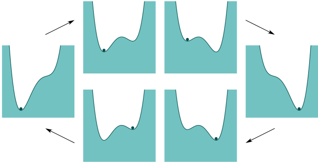
Figure 4: The potential $V(x,t)=\frac{1}{4}x^{4}-\frac{1}{2}x^{2}-\lambda(t)x$, with $\lambda(t)=K\cos(2\pi t)$, when $K$ exceeds the threshold $\lambda_{\mathchoice{\mbox{$\displaystyle\rm c$}}{\mbox{$\textstyle\rm c$}}{\mbox{$\scriptstyle\rm c$}}{\mbox{$\scriptscriptstyle\rm c$}}}$. In the deterministic case, with $\varepsilon\ll 1$, the overdamped particle jumps to a new well whenever $\lvert\lambda(t)\rvert$ becomes larger than $\lambda_{\mathchoice{\mbox{$\displaystyle\rm c$}}{\mbox{$\textstyle\rm c$}}{\mbox{$\scriptstyle\rm c$}}{\mbox{$\scriptscriptstyle\rm c$}}}$, leading to hysteresis. Larger values of $\varepsilon$ increase the size of hysteresis cycles, but additive noise of sufficient intensity decreases the size of typical cycles, because it advances transitions to the deeper well.

For positive $\varepsilon$, the system does not react immediately to changes in the potential, so that the hysteresis cycles are deformed. One can show [23, 10] that

• For $K\mathrel{\leqsymb}\lambda_{\mathchoice{\mbox{$\displaystyle\rm c$}}{\mbox{$\textstyle\rm c$}}{\mbox{$\scriptstyle\rm c$}}{\mbox{$\scriptscriptstyle\rm c$}}}+{\mathcal{O}}(\varepsilon)$, $x_{t}$ always tracks the same potential well, at a distance at most of order $\varepsilon/\sqrt{\lvert a_{0}\rvert}$ if $a_{0}\mathrel{\leqsymb}-\varepsilon$, and of order $\sqrt{\varepsilon}$ if $\lvert a_{0}\rvert$ is of order $\varepsilon$.

• For $K\mathrel{\geqsymb}\lambda_{\mathchoice{\mbox{$\displaystyle\rm c$}}{\mbox{$\textstyle\rm c$}}{\mbox{$\scriptstyle\rm c$}}{\mbox{$\scriptscriptstyle\rm c$}}}+{\mathcal{O}}(\varepsilon)$, $x_{t}$ is attracted by a hysteresis cycle, which is larger than the static hysteresis cycle; in particular, $x_{t}$ crosses the $\lambda$-axis when $\lambda(t)=K\cos 2\pi t=\lambda^{0}$, where $\lambda^{0}$ satisfies

  $$\lvert\lambda^{0}\rvert-\lambda_{\mathchoice{\mbox{$\displaystyle\rm c$}}{\mbox{$\textstyle\rm c$}}{\mbox{$\scriptstyle\rm c$}}{\mbox{$\scriptscriptstyle\rm c$}}}\asymp\varepsilon^{2/3}a_{0}^{1/3},\qquad\text{with $a_{0}=K-\lambda_{\mathchoice{\mbox{$\displaystyle\rm c$}}{\mbox{$\textstyle\rm c$}}{\mbox{$\scriptstyle\rm c$}}{\mbox{$\scriptscriptstyle\rm c$}}}$.}$$ (4.10)

Additive noise will also influence the shape of hysteresis cycles, because it can kick the state over the potential barrier, as has been noted in [28] in the context of the thermohaline circulation. For positive noise intensities $\sigma$, the value $\lambda^{0}$ at which $x_{t}$ crosses the $\lambda$-axis, becomes a random variable. Assume for instance that we start at time $t_{0}=1/4$ in the right-hand potential well. We define

$$\tau^{0}(\omega)=\inf\Bigl{\{}t\in\Bigl{[}\frac{1}{4},\frac{3}{4}\Bigr{]}\colon x_{t}(\omega)<0\Bigr{\}},\qquad\lambda^{0}(\omega)=\lambda(\tau^{0}(\omega)),$$ (4.11)

with the convention that $\tau^{0}(\omega)=\infty$ and $\lambda^{0}(\omega)=\infty$ if $x_{t}(\omega)>0$ for all $t\in[\frac{1}{4},\frac{3}{4}]$. We thus have $\tau^{0}\in[\frac{1}{4},\frac{3}{4}]\cup\{\infty\}$ and $\lambda^{0}\in[-K,K]\cup\{\infty\}$. We will indicate the parameter-dependence by $\lambda^{0}=\lambda^{0}(\varepsilon,\sigma)$, keeping in mind that this random variable also depends on $a_{0}$ and $\mu$. In the deterministic case, $\lambda^{0}(\varepsilon,0)=\infty$ if $K\mathrel{\leqsymb}\lambda_{\mathchoice{\mbox{$\displaystyle\rm c$}}{\mbox{$\textstyle\rm c$}}{\mbox{$\scriptstyle\rm c$}}{\mbox{$\scriptscriptstyle\rm c$}}}+{\mathcal{O}}(\varepsilon)$, and $\lambda^{0}(\varepsilon,0)$ satisfies (4.10) if $K\mathrel{\geqsymb}\lambda_{\mathchoice{\mbox{$\displaystyle\rm c$}}{\mbox{$\textstyle\rm c$}}{\mbox{$\scriptstyle\rm c$}}{\mbox{$\scriptscriptstyle\rm c$}}}+{\mathcal{O}}(\varepsilon)$.

As we know from the previous section, for $K<\lambda_{\mathchoice{\mbox{$\displaystyle\rm c$}}{\mbox{$\textstyle\rm c$}}{\mbox{$\scriptstyle\rm c$}}{\mbox{$\scriptscriptstyle\rm c$}}}$, there is an amplitude-dependent threshold noise level $\sigma_{\mathchoice{\mbox{$\displaystyle\rm c$}}{\mbox{$\textstyle\rm c$}}{\mbox{$\scriptstyle\rm c$}}{\mbox{$\scriptscriptstyle\rm c$}}}$ such that during one period, $x_{t}$ is unlikely to cross the potential barrier for $\sigma\ll\sigma_{\mathchoice{\mbox{$\displaystyle\rm c$}}{\mbox{$\textstyle\rm c$}}{\mbox{$\scriptstyle\rm c$}}{\mbox{$\scriptscriptstyle\rm c$}}}$, while it is likely to cross it for $\sigma\gg\sigma_{\mathchoice{\mbox{$\displaystyle\rm c$}}{\mbox{$\textstyle\rm c$}}{\mbox{$\scriptstyle\rm c$}}{\mbox{$\scriptscriptstyle\rm c$}}}$. In fact, in the latter case, there is a large probability to cross the barrier a time of order $\sigma^{2/3}$ before the instant $t=1/2$ of minimal barrier height, when $\lambda$ is of order $\lambda_{\mathchoice{\mbox{$\displaystyle\rm c$}}{\mbox{$\textstyle\rm c$}}{\mbox{$\scriptstyle\rm c$}}{\mbox{$\scriptscriptstyle\rm c$}}}-\sigma^{4/3}$. In that case, the hysteresis cycle will be smaller than the static cycle. A similar distinction between a small-noise and a large-noise regime exists for large-amplitude forcing.

It turns out that the distribution of $\lambda^{0}$ can be of three different types, depending on the values of the parameters (c.f. Figure 5 and Figure 6):

• Case I – Small-amplitude regime: $a_{0}\mathrel{\leqsymb}\text{{\it const }}\varepsilon$ and $\sigma\mathrel{\leqsymb}(\lvert a_{0}\rvert\vee\varepsilon)^{3/4}$.

  Then $x_{t}$ is unlikely to cross the potential barrier, and there are constants $C,\kappa>0$ such that (see [9, Theorem 2.3])

  $$\mathbb{P}\bigl{\{}\lambda^{0}<\infty\bigr{\}}\mathrel{\leqsymb}\frac{C}{\varepsilon}\operatorname{e}^{-\kappa(\lvert a_{0}\rvert\vee\varepsilon)^{3/2}/\sigma^{2}}.$$ (4.12)

  The probability to observe a “macroscopic” hysteresis cycle is very small, as most paths are concentrated in a small neighbourhood of the bottom of the right-hand potential well (Figure 5a).

  

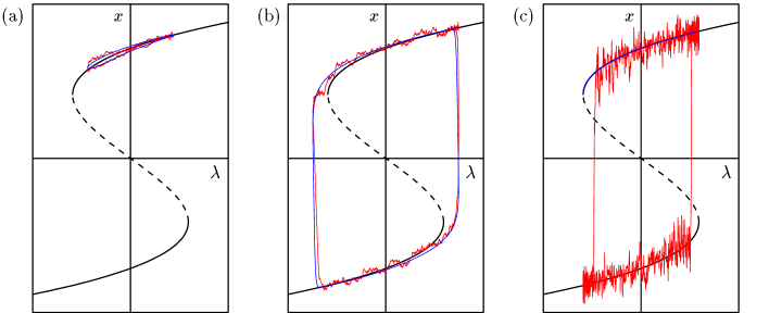
  Figure 5: Typical random hysteresis “cycles” in the three parameter regimes. (a) Case I: Driving amplitude $K$ and noise intensity $\sigma$ are too small to allow the path to switch potential wells. (b) Case II: For large amplitude but weak noise, the path tracks the deterministic hysteresis cycle, which is larger than the static one. (c) Case III: For sufficiently strong noise, the path can overcome the potential barrier, so that typical hysteresis cycles are smaller than the static one.

• Case II – Large-amplitude regime: $a_{0}\mathrel{\geqsymb}\text{{\it const }}\varepsilon$ and $\sigma\mathrel{\leqsymb}(\varepsilon\sqrt{a_{0}}\mskip 1.5mu)^{1/2}$.

  This regime is actually the most difficult to study, since the deterministic solution jumps when $\lvert\lambda(t)\rvert-\lambda_{\mathchoice{\mbox{$\displaystyle\rm c$}}{\mbox{$\textstyle\rm c$}}{\mbox{$\scriptstyle\rm c$}}{\mbox{$\scriptscriptstyle\rm c$}}}\asymp(\varepsilon\sqrt{a_{0}}\mskip 1.5mu)^{2/3}$, and crosses a zone of instability before reaching the left-hand potential well. One can show, however, that $\lvert\lambda^{0}\rvert$ is concentrated in an interval of length of order $(\varepsilon\sqrt{a_{0}}\mskip 1.5mu)^{2/3}$ around the deterministic value [9, Theorem 2.4]. More precisely, there are constants $C,\kappa>0$ such that

  $$\mathbb{P}\bigl{\{}\lvert\lambda^{0}\rvert<\lambda_{\mathchoice{\mbox{$\displaystyle\rm c$}}{\mbox{$\textstyle\rm c$}}{\mbox{$\scriptstyle\rm c$}}{\mbox{$\scriptscriptstyle\rm c$}}}-L\bigr{\}}\mathrel{\leqsymb}\frac{C}{\varepsilon}\operatorname{e}^{-\kappa L^{3/2}/\sigma^{2}}$$ (4.13)

  for $(\varepsilon\sqrt{a_{0}}\mskip 1.5mu)^{2/3}\mathrel{\leqsymb}L\mathrel{\leqsymb}L_{0}/\lvert\log(\varepsilon\sqrt{a_{0}}\mskip 1.5mu)\rvert$, and

  $$\mathbb{P}\bigl{\{}\lvert\lambda^{0}\rvert<\lambda_{\mathchoice{\mbox{$\displaystyle\rm c$}}{\mbox{$\textstyle\rm c$}}{\mbox{$\scriptstyle\rm c$}}{\mbox{$\scriptscriptstyle\rm c$}}}+L_{1}(\varepsilon\sqrt{a_{0}}\mskip 1.5mu)^{2/3}\bigr{\}}\mathrel{\leqsymb}\frac{C}{\varepsilon}\operatorname{e}^{-\kappa\varepsilon\sqrt{a_{0}}/\sigma^{2}},$$ (4.14)

  where the constants $L_{0},L_{1}>0$ are independent of the small parameters. Hence it is unlikely to observe a substantially smaller value of $\lvert\lambda^{0}\rvert$ than the deterministic one, provided $\sigma\ll(\varepsilon\sqrt{a_{0}}\mskip 1.5mu)^{1/2}$. On the other hand, there is a constant $L_{2}>L_{1}$ such that

  $$\mathbb{P}\bigl{\{}\lvert\lambda^{0}\rvert>\lambda_{\mathchoice{\mbox{$\displaystyle\rm c$}}{\mbox{$\textstyle\rm c$}}{\mbox{$\scriptstyle\rm c$}}{\mbox{$\scriptscriptstyle\rm c$}}}+L\bigr{\}}\mathrel{\leqsymb}3\operatorname{e}^{-\kappa L/(\sigma^{2}(\varepsilon\sqrt{a_{0}}\mskip 1.5mu)^{2/3}\lvert\log(\varepsilon\sqrt{a_{0}}\mskip 1.5mu)\rvert)}$$ (4.15)

  for all $L\mathrel{\geqsymb}L_{2}(\varepsilon\sqrt{a_{0}}\mskip 1.5mu)^{2/3}$. As a consequence, the vast majority of hysteresis cycles will look very similar to the deterministic ones, which are slightly larger than the static hysteresis cycle (Figure 5b).

  

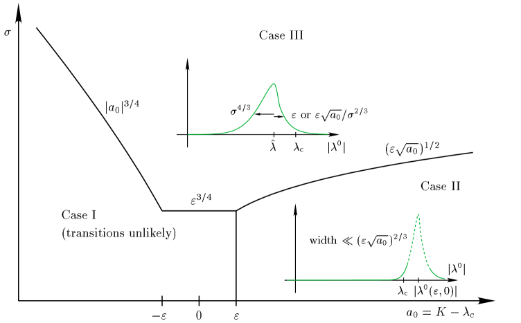
  Figure 6: The three hysteresis regimes, shown in the plane driving-amplitude–noise-intensity, for fixed driving frequency. The insets sketch the distribution of the random value $\lambda^{0}$ of the forcing $\lambda(t)$ when $x_{t}$ changes sign for the first time. In Case I, such transitions are unlikely. In Case II, $\lvert\lambda^{0}\rvert$ is concentrated in an interval $[\lambda_{\mathchoice{\mbox{$\displaystyle\rm c$}}{\mbox{$\textstyle\rm c$}}{\mbox{$\scriptstyle\rm c$}}{\mbox{$\scriptscriptstyle\rm c$}}}+L_{1}(\varepsilon\sqrt{a_{0}}\mskip 1.5mu)^{2/3},\lambda_{\mathchoice{\mbox{$\displaystyle\rm c$}}{\mbox{$\textstyle\rm c$}}{\mbox{$\scriptstyle\rm c$}}{\mbox{$\scriptscriptstyle\rm c$}}}+L_{2}(\varepsilon\sqrt{a_{0}}\mskip 1.5mu)^{2/3}]$ containing the deterministic value $\lvert\lambda^{0}(\varepsilon,0)\rvert$. The broken curve indicates that we do not control the distribution inside this interval. In Case III, $\lvert\lambda^{0}\rvert$ is concentrated around a value $\hat{\lambda}$ which is smaller than $\lambda_{\mathchoice{\mbox{$\displaystyle\rm c$}}{\mbox{$\textstyle\rm c$}}{\mbox{$\scriptstyle\rm c$}}{\mbox{$\scriptscriptstyle\rm c$}}}$ by an amount of order $\sigma^{4/3}$. The distribution decays faster to the right, with a width of order $\varepsilon$ (actually, $\varepsilon\lvert\log\sigma\rvert$) if $a_{0}\mathrel{\leqsymb}\varepsilon$ or $\sigma\mathrel{\geqsymb}\lvert a_{0}\rvert^{3/4}$, and of order $\varepsilon\sqrt{a_{0}}/\sigma^{2/3}$ if $a_{0}\mathrel{\geqsymb}\varepsilon$ and $\sigma\mathrel{\leqsymb}\lvert a_{0}\rvert^{3/4}$.

• Case III – Large-noise regime: Either $a_{0}\mathrel{\leqsymb}\varepsilon$ and $\sigma\mathrel{\geqsymb}(\lvert a_{0}\rvert\vee\varepsilon)^{3/4}$ or $a_{0}\mathrel{\geqsymb}\varepsilon$ and $\sigma\mathrel{\geqsymb}(\varepsilon\sqrt{a_{0}}\mskip 1.5mu)^{1/2}$.

  In this case, the noise is sufficiently strong to drive $x_{t}$ over the potential barrier, with large probability, some time before the barrier is lowest or vanishes, leading to a smaller hysteresis cycle than in the deterministic case (Figure 5c). It turns out that $\lvert\lambda^{0}\rvert$ is always concentrated around a (deterministic) value $\hat{\lambda}$ satisfying $\lambda_{\mathchoice{\mbox{$\displaystyle\rm c$}}{\mbox{$\textstyle\rm c$}}{\mbox{$\scriptstyle\rm c$}}{\mbox{$\scriptscriptstyle\rm c$}}}-\hat{\lambda}\asymp\sigma^{4/3}$. It follows from [9, Proposition 5.1] that

  $$\mathbb{P}\bigl{\{}\lvert\lambda^{0}\rvert<\hat{\lambda}-L\bigr{\}}\mathrel{\leqsymb}\frac{C}{\varepsilon}\operatorname{e}^{-\kappa L^{3/2}/\sigma^{2}}+\frac{3}{2}\operatorname{e}^{-\kappa\sigma^{4/3}/(\varepsilon\lvert\log\sigma\rvert)}$$ (4.16)

  for $0\mathrel{\leqsymb}L\mathrel{\leqsymb}\hat{\lambda}$ and

  $$\mathbb{P}\bigl{\{}\lvert\lambda^{0}\rvert>\hat{\lambda}+L\bigr{\}}\mathrel{\leqsymb}\frac{3}{2}\operatorname{e}^{-\kappa L/(\varepsilon\lvert\log\sigma\rvert)}$$ (4.17)

  for positive $L$ up to $K-\hat{\lambda}$ if $a_{0}\mathrel{\leqsymb}\varepsilon$. If $a_{0}\mathrel{\geqsymb}\varepsilon$, the same bound holds for $L\mathrel{\leqsymb}\lambda_{\mathchoice{\mbox{$\displaystyle\rm c$}}{\mbox{$\textstyle\rm c$}}{\mbox{$\scriptstyle\rm c$}}{\mbox{$\scriptscriptstyle\rm c$}}}-\hat{\lambda}$, while the behaviour for larger $L$ is described by (4.15). The estimates (4.16) and (4.17) hold if $a_{0}\mathrel{\leqsymb}\varepsilon$ or $\sigma>\smash{a_{0}^{3/4}}$. In the other case, two exponents are modified: $\sigma^{4/3}/(\varepsilon\lvert\log\sigma\rvert)$ is replaced by $\sigma^{2}/(\varepsilon\sqrt{a_{0}}\mskip 1.5mu\lvert\log\sigma\rvert)$, and $L/(\varepsilon\lvert\log\sigma\rvert)$ is replaced by $\sigma^{2/3}L/(\varepsilon\sqrt{a_{0}}\mskip 1.5mu\lvert\log\sigma\rvert)$.

  Note that in all cases, the distribution of $\lambda^{0}$ decays faster to the right than to the left of $\hat{\lambda}$, and it is unlikely to observe $\lambda^{0}$ larger than $\lambda_{\mathchoice{\mbox{$\displaystyle\rm c$}}{\mbox{$\textstyle\rm c$}}{\mbox{$\scriptstyle\rm c$}}{\mbox{$\scriptscriptstyle\rm c$}}}$, except when approaching the lower boundary of Region III.

In some physical applications, for instance in ferromagnets, the area enclosed by hysteresis cycles represents the energy dissipation per period. The distribution of the random hysteresis area can also be described, and bounds on its expectation and variance can be obtained. We refer to [9] and [8, Section 4] for details.

For Stommel’s box model, the above properties have two important consequences. First, noise can drive the system from one stable equilibrium to the other before the potential barrier between them disappears, so that a smaller deviation from the mean freshwater flux than expected from the deterministic analysis can switch the system’s state. Second, this early switching to the other state is likely only if the noise intensity exceeds a threshold value (which is lowest when the amplitude $K$ is close to $\lambda_{\mathchoice{\mbox{$\displaystyle\rm c$}}{\mbox{$\textstyle\rm c$}}{\mbox{$\scriptstyle\rm c$}}{\mbox{$\scriptscriptstyle\rm c$}}}$). Still, the system spends roughly half of the time per period in metastable equilibrium in the shallower well.

5 Delay

Convective motions in the atmosphere can be simulated in a laboratory experiment known as Rayleigh–Bénard convection. A fluid contained between two horizontal plates is heated from below. For low heating, the fluid remains at rest. Above a threshold, stationary convection rolls develop. With increasing energy supply, the angular velocity of the rolls becomes time-dependent, first periodically, and then, after a sequence of bifurcations depending on the geometry of the set-up, chaotic. For still stronger heating, the convection rolls are destroyed and the dynamics becomes turbulent.

Lorenz’ famous model [26] uses a three-modes Galerkin approximation of the hydrodynamic equations. The amplitudes of these modes obey the ODEs

$$\begin{split}\dot{X}&=\mathchoice{\mbox{$\displaystyle\rm Pr$}}{\mbox{$\textstyle\rm Pr$}}{\mbox{$\scriptstyle\rm Pr$}}{\mbox{$\scriptscriptstyle\rm Pr$}}(Y-X)\\ \dot{Y}&=rX-Y-XZ\\ \dot{Z}&=-bZ+XY.\end{split}$$ (5.1)

Here $X$ measures the angular velocity of convection rolls, while $Y$ and $Z$ parametrize the temperature field. The Prandtl number $\mathchoice{\mbox{$\displaystyle\rm Pr$}}{\mbox{$\textstyle\rm Pr$}}{\mbox{$\scriptstyle\rm Pr$}}{\mbox{$\scriptscriptstyle\rm Pr$}}>0$ is a characteristic of the fluid, $b$ depends on the geometry of the container, and $r$ is proportional to the heating.

For $0\mathrel{\leqsymb}r\mathrel{\leqsymb}1$, the origin $(X,Y,Z)=(0,0,0)$ is a global attractor of the system, corresponding to the fluid at rest. At $r=1$, this state becomes unstable in a pitchfork bifurcation. Two new stable equilibrium branches $(\pm\sqrt{b(r-1)},\pm\sqrt{b(r-1)},r-1)$ are created, which correspond to convection rolls with the two possible directions of rotation. We will focus on this simplest bifurcation, ignoring all the other sequences of bifurcations ultimately leading to a strange attractor (see for instance [32]).

We are interested in the situation where $r=r(\varepsilon t)$ grows monotonously through $r(0)=1$ with low speed $\varepsilon$ (e.g. $r=1+\varepsilon t$). Near the bifurcation point, one can reduce the system to an invariant center manifold, on which the dynamics is governed (c.f. [10]), after scaling time by a factor $\varepsilon$, by the one-dimensional equation

$$\varepsilon\frac{\operatorname{d}\!x}{\operatorname{d}\!t}=\mu(t)x+c(t)x^{3}+{\mathcal{O}}(x^{5}).$$ (5.2)

Here $\mu(t)=a(t)+{\mathcal{O}}(\varepsilon)$, where $a(t)=\frac{1}{2}\bigl{[}-(\mathchoice{\mbox{$\displaystyle\rm Pr$}}{\mbox{$\textstyle\rm Pr$}}{\mbox{$\scriptstyle\rm Pr$}}{\mbox{$\scriptscriptstyle\rm Pr$}}+1)+\sqrt{(\mathchoice{\mbox{$\displaystyle\rm Pr$}}{\mbox{$\textstyle\rm Pr$}}{\mbox{$\scriptstyle\rm Pr$}}{\mbox{$\scriptscriptstyle\rm Pr$}}+1)^{2}+4\mathchoice{\mbox{$\displaystyle\rm Pr$}}{\mbox{$\textstyle\rm Pr$}}{\mbox{$\scriptstyle\rm Pr$}}{\mbox{$\scriptscriptstyle\rm Pr$}}(r(t)-1)}\mskip 1.5mu\bigr{]}$ is the largest eigenvalue of the linearization of (5.1) at $0$, which has the same sign as $r(t)-1$, and $c(t)$ is negative and bounded away from zero. The right-hand side of (5.2) derives from a potential similar to the Ginzburg–Landau potential (1.8) with $\lambda=0$, which remains symmetric while transforming from a single-well to a double-well as $\mu(t)$ becomes positive, see Figure 7.

Figure 7: The potential $V(x,t)=\frac{1}{4}x^{4}-\tfrac{1}{2}\mu(t)x^{2}$ transforms, as $\mu$ changes from negative to positive, from a single-well to a double-well potential. In the deterministic case, an overdamped particle stays close to the saddle for a macroscopic time before falling into one of the wells. Noise tends to reduce this delay.

The solution of (5.2) with initial condition $x_{0}>0$ for $t_{0}<0$ can be written in the form

$$x_{t}=\varphi(x_{0},t)\operatorname{e}^{\alpha(t,t_{0})/\varepsilon},\qquad\qquad\alpha(t,t_{0})=\int_{t_{0}}^{t}\mu(s)\operatorname{d}\!s,$$ (5.3)

with $0<\varphi(x_{0},t)\mathrel{\leqsymb}x_{0}$ for all $t$. Thus $x_{t}$ is exponentially small if $\alpha(t,t_{0})$ is negative. The important point to note is that $\alpha(t,t_{0})$ can be negative even when $a(t)$ is positive. For instance, if $\mu(s)=s$, then $\alpha(t,t_{0})=\frac{1}{2}(t^{2}-t_{0}^{2})$ is negative for $t_{0}<t<-t_{0}$. Thus $x_{t}$ will remain exponentially close to the saddle at $x=0$ up to time $-t_{0}$ after crossing the bifurcation point. This phenomenon is called bifurcation delay. It means that when $r$ is slowly increased, convection rolls will not appear at $r=1$, as expected from the static analysis, but only for some larger value of $r$, which depends on the initial condition.

It is clear that the existence of a delay depends crucially on the fact that $x_{t}$ can approach the saddle exponentially closely, where the repulsion is very small. Noise present in the system will help kicking $x_{t}$ away from the saddle, and thus reduce the delay. The question is to determine how the delay depends on the noise intensity $\sigma$.

For brevity, we will illustrate the results in the particular case of a Ginzburg–Landau potential, with dynamics governed by the SDE

$$\operatorname{d}\!x_{t}=\frac{1}{\varepsilon}\bigl{[}\mu(t)x_{t}-x_{t}^{3}\bigr{]}\operatorname{d}\!t+\frac{\sigma}{\sqrt{\varepsilon}}\operatorname{d}\!W_{t}.$$ (5.4)

The case without the term $-x_{t}^{3}$ has been analysed by several authors [38, 33, 35, 22], with the result that the typical bifurcation delay in the presence of noise behaves like $\sqrt{\lvert\log\sigma\rvert}$. The results in [6] cover more general nonlinearities than $-x^{3}$.

We assume that $\mu(t)$ is increasing, and satisfies $\mu(0)=0$, $\mu^{\prime}(0)\mathrel{\geqsymb}\text{{\it const }}>0$. For simplicity, we consider first the case where $x_{t}$ starts at a time $t_{0}<0$ at the origin $x=0$. From the results of Section 2, we expect the paths to remain concentrated, for some time, in a set whose width is related to the linearization of (5.4) around $x=0$. We define the function

$$\bar{v}(t)=\bar{v}_{0}\operatorname{e}^{2\alpha(t)/\varepsilon}+\frac{\sigma^{2}}{\varepsilon}\int_{t_{0}}^{t}\operatorname{e}^{2\alpha(t,s)/\varepsilon}\operatorname{d}\!s,\qquad\text{where $\alpha(t)=\alpha(t,0)$.}$$ (5.5)

For a suitably chosen $\bar{v}_{0}\asymp\sigma^{2}/\lvert\mu(t_{0})\rvert$, one can show that $\bar{v}(t)$ is increasing and satisfies

$$\bar{v}(t)\asymp\begin{cases}{\sigma^{2}}/{\lvert\mu(t)\rvert}&\text{for $t_{0}\mathrel{\leqsymb}t\mathrel{\leqsymb}-\sqrt{\varepsilon}$}\\ {\sigma^{2}}/{\sqrt{\varepsilon}}&\text{for $-\sqrt{\varepsilon}\mathrel{\leqsymb}t\mathrel{\leqsymb}\sqrt{\varepsilon}$}\\ {\sigma^{2}}\operatorname{e}^{2\alpha(t)/\varepsilon}/{\sqrt{\varepsilon}}&\text{for $t\mathrel{\geqsymb}\sqrt{\varepsilon}$.}\end{cases}$$ (5.6)

Note that although the curvature $\lvert\mu(t)\rvert$ of the potential at the origin vanishes at time $0$, $\bar{v}(t)$ grows slowly until time $\sqrt{\varepsilon}$ after the bifurcation point, and only then it starts growing faster and faster.

We now introduce, as in Section 2, the set

$${\mathcal{B}}(h)=\bigl{\{}(x,t)\colon\lvert x\rvert\mathrel{\leqsymb}h\sqrt{\bar{v}(t)}\mskip 1.5mu\bigr{\}}.$$ (5.7)

Then one can show (see [6, Theorem 2.10]) the existence of a constant $h_{0}>0$ such that the first-exit time $\tau_{{\mathcal{B}}(h)}$ of $x_{t}$ from ${\mathcal{B}}(h)$ satisfies

$$\mathbb{P}\bigl{\{}\tau_{{\mathcal{B}}(h)}<t\bigr{\}}\mathrel{\leqsymb}C(t,\varepsilon)\operatorname{e}^{-\kappa h^{2}}$$ (5.8)

for all $h\mathrel{\leqsymb}h_{0}\sigma/\bar{v}(t)$, where

$$C(t,\varepsilon)=\frac{1}{\varepsilon^{2}}\int_{t_{0}}^{t}\lvert\mu(s)\rvert\operatorname{d}\!s+{\mathcal{O}}\biggl{(}\frac{1}{\varepsilon}\biggr{)},\qquad\text{and}\qquad\kappa=\frac{1}{2}-{\mathcal{O}}(\sqrt{\varepsilon}\mskip 1.5mu)-{\mathcal{O}}\biggl{(}\frac{h^{2}\bar{v}(t)^{2}}{\sigma^{2}}\biggr{)}.$$ (5.9)

The paths are concentrated in ${\mathcal{B}}(h)$, provided $h_{0}^{2}\sigma^{2}/\bar{v}(t)^{2}\mathrel{\geqsymb}h^{2}\gg\log C(t,\varepsilon)$. As a consequence, we can distinguish between three regimes, depending on noise intensity:

• Regime I: $\sigma\mathrel{\leqsymb}\operatorname{e}^{-K/\varepsilon}$ for some $K>0$.

  The paths are concentrated near $x=0$ at least as long as $2\alpha(t)\ll K$. This implies that there is still a macroscopic bifurcation delay.

• Regime II: $\operatorname{e}^{-1/\varepsilon^{p}}\mathrel{\leqsymb}\sigma\ll\sqrt{\varepsilon}$ for some $p<1$.

  The paths are concentrated near $x=0$ at least up to time $\sqrt{\varepsilon}$, with a typical spreading growing like $\sigma/\sqrt{\lvert\mu(t)\rvert}$ for $t\mathrel{\leqsymb}-\sqrt{\varepsilon}$, and remaining of order $\sigma/\varepsilon^{1/4}$ for $\lvert t\rvert\mathrel{\leqsymb}\sqrt{\varepsilon}$.

• Regime III: $\sigma\mathrel{\geqsymb}\sqrt{\varepsilon}$.

  The paths are concentrated near $x=0$ at least up to time $-\sigma$, with a typical spreading growing like $\sigma/\sqrt{\lvert\mu(t)\rvert}$. Near $t=0$, the potential becomes too flat to counteract the diffusion, and as $t$ grows further, paths keep switching back and forth between the wells, before ultimately settling for a well.

Similar results hold if $x_{t}$ starts, at $t_{0}<0$, away from $x=0$, say in $x_{0}>0$. Then the set ${\mathcal{B}}(h)$ is centred at the deterministic solution $x^{\det}_{t}$ (with the same initial condition), which jumps to the right-hand well when $\alpha(t,t_{0})$ becomes positive, see Figure 8. In Regime I, with $K$ sufficiently large, the majority of paths follow $x^{\det}_{t}$ into the right-hand potential well.

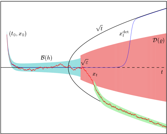
Figure 8: A sample path $x_{t}$ of the SDE (5.4) with $\mu(t)=t$, for $\varepsilon=0.01$ and $\sigma=0.015$. The deterministic solution $x^{\det}_{t}$, starting in $x_{0}>0$ at time $t_{0}$, jumps to the right-hand well, located at $x^{\star}(t)=\sqrt{t}$, at time $\lvert t_{0}\rvert$. Typical paths stay in the set ${\mathcal{B}}(h)$, whose width increases like $h\sigma/(\sqrt{\lvert t\rvert}\vee\varepsilon^{1/4})$, until time $\sqrt{\varepsilon}$ after the bifurcation. They leave the domain ${\mathcal{D}}(\varrho)$ (shown for $\varrho=2/3$) at a random time $\tau=\tau_{{\mathcal{D}}(\varrho)}$, which is typically of order $\smash{\sqrt{\varepsilon{\lvert\log\sigma\rvert}}}$. After leaving ${\mathcal{D}}(\varrho)$, each path is likely to stay in a strip of width of order $h\sigma/\sqrt{t}$, centred at a deterministic solution approaching either $+x^{\star}(t)$ or $-x^{\star}(t)$.

It remains to understand the behaviour after time $\sqrt{\varepsilon}$ in Regime II. To this end, we introduce the set

$${\mathcal{D}}(\varrho)=\bigl{\{}(x,t)\colon t\mathrel{\geqsymb}\sqrt{\varepsilon},\lvert x\rvert\mathrel{\leqsymb}\sqrt{(1-\varrho)\mu(t)}\mskip 1.5mu\bigr{\}},$$ (5.10)

depending on a parameter $\varrho\in[0,2/3)$. The set ${\mathcal{D}}(0)$ contains the points lying between the two stable equilibrium branches $\pm\sqrt{\mu(t)}$. One can show (see [6, Theorem 2.11]) that if $\varrho\in(0,2/3)$ and $\sigma\lvert\log\sigma\rvert^{3/2}={\mathcal{O}}(\sqrt{\varepsilon}\mskip 1.5mu)$, then the first-exit time $\tau_{{\mathcal{D}}(\varrho)}$ of $x_{t}$ from ${\mathcal{D}}(\varrho)$ satisfies

$$\mathbb{P}\bigl{\{}\tau_{{\mathcal{D}}(\varrho)}\mathrel{\geqsymb}t\bigr{\}}\mathrel{\leqsymb}C(t,\varepsilon)\frac{\lvert\log\sigma\rvert}{\sigma}\frac{\operatorname{e}^{-\varrho\alpha(t,\sqrt{\varepsilon}\mskip 1.5mu)/\varepsilon}}{\sqrt{1-\operatorname{e}^{-2\varrho\alpha(t,\sqrt{\varepsilon}\mskip 1.5mu)/\varepsilon}}},$$ (5.11)

where

$$C(t,\varepsilon)=\text{{\it const }}\mu(t)\biggl{(}1+\frac{\alpha(t,\sqrt{\varepsilon}\mskip 1.5mu)}{\varepsilon}\biggr{)}.$$ (5.12)

The estimate (5.11) shows that paths are unlikely to stay in ${\mathcal{D}}(\varrho)$ as soon as $t$ satisfies $\varrho\alpha(t,\sqrt{\varepsilon}\mskip 1.5mu)\gg\varepsilon\lvert\log\sigma\rvert$. Since $\alpha$ is quadratic in $t$, most paths will have left ${\mathcal{D}}(\varrho)$ for

$$t\gg\sqrt{\varepsilon\lvert\log\sigma\rvert}.$$ (5.13)

Once $x_{t}$ has left ${\mathcal{D}}(\varrho)$, one can further show that it is likely to track a deterministic solution which approaches the bottom of one of the potential wells. Assume for instance that $x_{t}$ leaves ${\mathcal{D}}(\varrho)$ through the upper boundary, at a random time $\tau=\tau_{{\mathcal{D}}(\varrho)}$. Then, for $1/2<\varrho<2/3$, [6, Theorem 2.12] shows that the deterministic solution $x^{\det,\tau}_{t}$, starting in the same point at time $\tau$, approaches the bottom of the well at $\sqrt{\mu(t)}$ like $\varepsilon/\mu(t)^{3/2}+\sqrt{\mu(\tau)}\operatorname{e}^{-\eta\alpha(t,\tau)/\varepsilon}$, where $\eta=2-3\varrho$, and the path $x_{t}$ is likely to stay in a strip of width $\sigma/\sqrt{\mu(t)}$ around $x^{\det,\tau}$. Thus after another time span of the form (5.13), most paths will have concentrated near the bottom of a potential well again.

We note that different kinds of metastability play a rôle here. First, paths remain concentrated for some time near the unstable saddle. Second, they will concentrate again near one of the potential wells after some time. Some paths will choose the left-hand well and others the right-hand well (with probability exponentially close to $1/2$ in Regime II), but all the paths which choose a given potential well are unlikely to cross the barrier again. In fact, one can show that if $\mu(t)$ grows at least linearly, then the probability ever to cross the saddle again is of order $\operatorname{e}^{-\text{{\it const}}/\sigma^{2}}$. If we start the system at a positive $t_{0}$ in one of the wells, the distribution will never approach a symmetric bimodal one.

In the case of the Rayleigh–Bénard convection with slowly growing heat supply $r(\varepsilon t)$ and additive noise, these results mean that exponentially weak noise will not prevent the delayed appearance of convection rolls. For moderate noise intensity, rolls will appear after a delay of order $\sqrt{\lvert\log\sigma\rvert/\varepsilon}$, which is considerably shorter than the delay in the deterministic case which is of order $1/\varepsilon$. The direction of rotation is unlikely to change after another time span of that order. For strong noise, convection rolls may appear early, but their angular velocity will fluctuate around zero until a time of order $\sigma/\varepsilon$ after the bifurcation before settling for a sign, and even then occasional changes of rotation direction are possible.

Acknowledgements

We thank the organisers for the invitation to Chorin and the opportunity to present our results during the Second Workshop on Stochastic Climate Models. We enjoyed stimulating discussions in a pleasant atmosphere.

Nils Berglund
Department of Mathematics, ETH Zürich
ETH Zentrum, 8092 Zürich, Switzerland
E-mail address: berglund@math.ethz.ch

Barbara Gentz
Weierstraß Institute for Applied Analysis and Stochastics
Mohrenstraße 39, 10117 Berlin, Germany
E-mail address: gentz@wias-berlin.de

References

• [1] L. Arnold. Random Dynamical Systems. Springer-Verlag, Berlin, 1998.
• [2] L. Arnold. Hasselmann’s program revisited: The analysis of stochasticity in deterministic climate models. In P. Imkeller and J.-S. von Storch, editors, Stochastic Climate Models, volume 49 of Progress in Probability, pages 141–158, Boston, 2001. Birkhäuser.
• [3] R. Azencott. Petites perturbations aléatoires des systèmes dynamiques: développements asymptotiques. Bull. Sci. Math. (2), 109:253–308, 1985.
• [4] R. Benzi, G. Parisi, A. Sutera, and A. Vulpiani. A theory of stochastic resonance in climatic change. SIAM J. Appl. Math., 43(3):565–578, 1983.
• [5] N. Berglund and B. Gentz. In preparation.
• [6] N. Berglund and B. Gentz. Pathwise description of dynamic pitchfork bifurcations with additive noise. To appear in Probab. Theory Related Fields.
Available at http://arXiv.org/abs/math.PR/0008208, 2000.
• [7] N. Berglund and B. Gentz. A sample-paths approach to noise-induced synchronization: Stochastic resonance in a double-well potential. Submitted.
Available at http://arXiv.org/abs/math.PR/0012267, 2000.
• [8] N. Berglund and B. Gentz. Beyond the Fokker–Planck equation: Pathwise control of noisy bistable systems. Submitted. Available at http://arXiv.org/abs/cond-mat/0110180, 2001.
• [9] N. Berglund and B. Gentz. The effect of additive noise on dynamical hysteresis. Submitted. Available at http://arXiv.org/abs/math.DS/0107199, 2001.
• [10] N. Berglund and H. Kunz. Memory effects and scaling laws in slowly driven systems. J. Phys. A, 32(1):15–39, 1999.
• [11] P. Cessi. A simple box model of stochastically forced thermohaline flow. J. Phys. Oceanogr., 24:1911–1920, 1994.
• [12] H. Crauel and F. Flandoli. Attractors for random dynamical systems. Probab. Theory Related Fields, 100(3):365–393, 1994.
• [13] H. Crauel and F. Flandoli. Additive noise destroys a pitchfork bifurcation. J. Dynam. Differential Equations, 10(2):259–274, 1998.
• [14] M. V. Day. On the exponential exit law in the small parameter exit problem. Stochastics, 8:297–323, 1983.
• [15] W. H. Fleming and M. R. James. Asymptotic series and exit time probabilities. Ann. Probab., 20(3):1369–1384, 1992.
• [16] R. F. Fox. Stochastic resonance in a double well. Phys. Rev. A, 39:4148–4153, 1989.
• [17] M. I. Freidlin. Quasi-deterministic approximation, metastability and stochastic resonance. Physica D, 137:333–352, 2000.
• [18] M. I. Freidlin and A. D. Wentzell. Random Perturbations of Dynamical Systems. Springer-Verlag, New York, second edition, 1998.
• [19] I. S. Gradšteĭn. Application of A. M. Lyapunov’s theory of stability to the theory of differential equations with small coefficients in the derivatives. Mat. Sbornik N. S., 32(74):263–286, 1953.
• [20] K. Hasselmann. Stochastic climate models. Part I. Theory. Tellus, 28:473–485, 1976.
• [21] W. Horsthemke and R. Lefever. Noise-induced transitions. Springer-Verlag, Berlin, 1984.
• [22] K. M. Jansons and G. D. Lythe. Stochastic calculus: application to dynamic bifurcations and threshold crossings. J. Statist. Phys., 90(1–2):227–251, 1998.
• [23] P. Jung, G. Gray, R. Roy, and P. Mandel. Scaling law for dynamical hysteresis. Phys. Rev. Letters, 65:1873–1876, 1990.
• [24] P. Jung and P. Hänggi. Stochastic nonlinear dynamics modulated by external periodic forces. Europhys. Letters, 8:505–510, 1989.
• [25] Y. Kifer. The exit problem for small random perturbations of dynamical systems with a hyperbolic fixed point. Israel J. Math., 40(1):74–96, 1981.
• [26] E. N. Lorenz. Deterministic nonperiodic flow. J. Atmos. Sciences, 20:130–141, 1963.
• [27] B. McNamara and K. Wiesenfeld. Theory of stochastic resonance. Phys. Rev. A, 39:4854–4869, 1989.
• [28] A. H. Monahan. Stabilisation of climate regimes by noise in a simple model of the thermohaline circulation. Preprint, 2001.
• [29] F. Moss and K. Wiesenfeld. The benefits of background noise. Scientific American, 273:50–53, 1995.
• [30] S. Rahmstorf. Bifurcations of the Atlantic thermohaline circulation in response to changes in the hydrological cycle. Nature, 378:145–149, 1995.
• [31] B. Schmalfuß. Invariant attracting sets of nonlinear stochastic differential equations. In H. Langer and V. Nollau, editors, Markov processes and control theory, volume 54 of Math. Res., pages 217–228, Berlin, 1989. Akademie-Verlag. Gaußig, 1988.
• [32] C. Sparrow. The Lorenz Equations: Bifurcations, Chaos and Strange Attractors. Springer-Verlag, New York, 1982.
• [33] N. G. Stocks, R. Manella, and P. V. E. McClintock. Influence of random fluctuations on delayed bifurcations: The case of additive white noise. Phys. Rev. A, 40:5361–5369, 1989.
• [34] H. Stommel. Thermohaline convection with two stable regimes of flow. Tellus, 13:224–230, 1961.
• [35] J. B. Swift, P. C. Hohenberg, and G. Ahlers. Stochastic Landau equation with time-dependent drift. Phys. Rev. A, 43:6572–6580, 1991.
• [36] A. N. Tihonov. Systems of differential equations containing small parameters in the derivatives. Mat. Sbornik N. S., 31:575–586, 1952.
• [37] T. Tomé and M. J. de Oliveira. Dynamic phase transition in the kinetic Ising model under a time-dependent oscillating field. Phys. Rev. A, 41:4251–4254, 1990.
• [38] M. C. Torrent and M. San Miguel. Stochastic-dynamics characterization of delayed laser threshold instability with swept control parameter. Phys. Rev. A, 38:245–251, 1988.
• [39] K. Wiesenfeld and F. Moss. Stochastic resonance and the benefits of noise: from ice ages to crayfish and SQUIDs. Nature, 373:33–36, 1995.