A Discrete Four Stroke Quantum Heat Engine Exploring the Origin of Friction.

Abstract

The optimal power performance of a first principle quantum heat engine model shows friction-like phenomena when the internal fluid Hamiltonian does not commute with the external control field. The model is based on interacting two-level-systems where the external magnetic field serves as a control variable.

I Introduction

It is well established that the performance of working heat engines are limited by intrinsic unavoidable irreversibilities. Maximum power is obtained at the expense of efficiency where the reversible point of maximum efficiency has zero power. This principle has been clearly illustrated by the endoreversible model of Curzon and Ahlborn [2] and summarized by Salamon et. al. [3]. Two additional unavoidable sources of loss are heat leaks which practically eliminate the maximum efficiency adiabatic operation, and internal friction which restricts fast operating cycles.

Is this universal performance limitation of heat engines macroscopic or microscopic? Though the common image of heat engines is of large macroscopic devices, microscopic models based on first principle quantum mechanics are limited by the Carnot efficiency [5], and show a remarkable resemblance to their macroscopic analogs when the engines produce finite power [4].

In previous studies, both discrete [6, 7, 8, 9, 10] and continuous quantum models [4, 11, 12, 13] have been scrutinized, which are analogous, respectively, to four-stroke-engines and turbines. The present study examines a discrete four-stroke quantum engine, comparing it to an engine subject to phenomenological internal friction. It will be demonstrated that the quantum engines inability to control simultaneously the external and internal portions of the working fluid Hamiltonian is its source of friction.

II Basic construction

All working heat engines and all refrigerators operate on the same principle. The engine manipulates the energy flow between three reservoirs, a hot, cold and power reservoir, either to extract power from the temperature difference or to pump heat from the cold to the hot reservoir at the expense of external power.

The present model of a discrete quantum heat engine is composed of a cycle of operation constructed from two adiabats and two isotherms similar to a Otto cycle. The quantum dynamics are generated by external fields in the adiabats and by heat flows from hot and cold reservoirs in the isochores. The working medium is modeled as a gas of interacting particles with the Hamiltonian:

$${\bf\hat{H}}~{}~{}=~{}~{}{\bf\hat{H}_{ext}}~{}+~{}{\bf\hat{H}_{int}}~{}~{}.$$ (1)

${\bf\hat{H}_{ext}}=\omega\sum_{i}{\bf\hat{H}_{i}}$ is the sum of single particle Hamiltonians, $\omega=\omega(t)$ is the time dependent external control field, and ${\bf\hat{H}_{int}}$ represents the inter-particle interaction.

The change in time of an operator ${\bf\hat{A}}$ during the adiabatic/isochoreal branches is described as:

$$\dot{\bf\hat{A}}~{}~{}=~{}~{}i[{\bf\hat{H}},{\bf\hat{A}}]~{}+~{}\frac{\partial{\bf\hat{A}}}{\partial t}~{}~{}+~{}~{}{\cal L}_{D}({\bf\hat{A}})~{}~{}~{},$$ (2)

${\cal L}_{D}$ represents the Liouville dissipative generator on the isochore in contact with either the hot or cold bath (units of $\hbar=1$). Replacing ${\bf\hat{A}}$ by ${\bf\hat{H}}$ in Eq. (2) leads to the power invested in or extracted from the adiabats:,

$${\cal P}~{}~{}=~{}~{}\dot{\omega}\sum_{i}\langle{\bf\hat{H}_{i}}\rangle~{}~{}~{},$$ (3)

where $\langle{\bf\hat{H}_{i}}\rangle$ is the expectation value of the single particle Hamiltonian. The heat flow is extracted from the energy balance on the isochores [4, 10]:

$$\dot{\cal Q}_{h/c}~{}~{}=~{}~{}\langle{\cal L}_{h/c}\left({\bf\hat{H}}\right)\rangle~{}~{}.$$ (4)

For simplicity, the single particle Hamiltonian is chosen as a two-level-system (TLS): ${\bf\hat{H}}_{i}={\boldsymbol{\mathrm{\hat{\sigma}}}}_{z}^{i}$. The interaction term is restricted to coupling of pairs of spin atoms. As a result, the state of the working medium is described by an ensemble of pairs of two-level-systems represented by the density operator $\hat{\rho}$, defined in the tensor product space of the individual two TLS systems. Expectation values are obtained by the usual definition $\langle{\bf\hat{A}}\rangle=tr\{{\bf\hat{A}}\hat{\rho}\}$. The external Hamiltonian then becomes:

$${\bf\hat{H}_{ext}}~{}~{}=~{}~{}\omega\left({\boldsymbol{\mathrm{\hat{\sigma}}}}_{z}^{1}\otimes{\bf\hat{I}^{2}}+{\bf\hat{I}^{1}}\otimes\hat{\sigma}_{z}^{2}\right)$$ (5)

and the external field is chosen to be in the $z$ direction. The interaction Hamiltonian is chosen as:

$${\bf\hat{H}_{int}}~{}~{}=~{}~{}J\left({{\boldsymbol{\mathrm{\hat{\sigma}}}}_{x}^{1}}\otimes{{\boldsymbol{\mathrm{\hat{\sigma}}}}_{x}^{2}}-{{\boldsymbol{\mathrm{\hat{\sigma}}}}_{y}^{1}}\otimes{\boldsymbol{\mathrm{\hat{\sigma}}}}_{y}^{2}\right)~{}~{}.$$ (6)

$J$ scales the strength of the interaction. When $J\rightarrow 0$ the model approaches the previously studied frictionless model [8]. The inter-particle interaction term, Eq. (6), defines a correlation energy between the two single particle spins in the $\vec{x}$ and $\vec{y}$ direction. As a result, $[{\bf\hat{H}_{ext}},{\bf\hat{H}_{int}}]\neq 0$, since the external Hamiltonian is polarized in the $\vec{z}$ direction.

III Dynamics of the working medium

The dynamics generated by the Hamiltonian is completely determined by the algebra of commutation relations of the set of 16 operators spanning the Hilbert space of the combined system. Due to symmetry, the commutation algebra decomposes into subsets of operators with closed commutation relations. The set is generated by commutation relations between the operators composing the Hamiltonian:

$$\begin{array}[]{c}{\bf\hat{B}}_{1}\end{array}= ~{}~{}~{}\begin{array}[]{c}{\boldsymbol{\mathrm{\hat{\sigma}}}}_{z}^{1}\otimes{\bf\hat{I}^{2}}~{}+~{}{\bf\hat{I}^{1}}\otimes{\boldsymbol{\mathrm{\hat{\sigma}}}}_{z}^{2}\end{array}~{}~{}~{}~{},~{}~{}~{}~{}$$ (9)

$$\begin{array}[]{c}{\bf\hat{B}}_{2}\end{array}= \begin{array}[]{c}{{\boldsymbol{\mathrm{\hat{\sigma}}}}_{x}^{1}}\otimes{{\boldsymbol{\mathrm{\hat{\sigma}}}}_{x}^{2}}-{{\boldsymbol{\mathrm{\hat{\sigma}}}}_{y}^{1}}\otimes{{\boldsymbol{\mathrm{\hat{\sigma}}}}_{y}^{2}}\end{array}~{}~{}~{}~{}.$$ (12)

The commutation relation: $[{\bf\hat{B}}_{1},{\bf\hat{B}}_{2}]=4i{\bf\hat{B}}_{3}$ leads to the definition of ${\bf\hat{B}}_{3}$ which closes the set i.e. the set of operators ${\bf\hat{B}}_{1},{\bf\hat{B}}_{2},{\bf\hat{B}}_{3}$ forms a closed subset of the Lie algebra of the combined system. The Hamiltonian expressed in terms of the set of operators becomes: ${\bf\hat{H}}~{}=~{}\omega{\bf\hat{B}_{1}}+\rm J{\bf\hat{B}_{2}}$

The commutation relations of the set of $\bf\hat{B}_{i}$ operators are isomorphic to the angular momentum commutation relations when the transformation $\frac{1}{4}{\bf\hat{B}_{\rm i}}~{}\rightarrow~{}{\bf\hat{J}_{\rm i}}$ is applied. This similarity can be exploited to express the expectation values in a Cartesian three dimensional space, where the external field is in the $\bf B_{1}$ or $\vec{z}$ direction, the correlations in the $\bf B_{2}$ or $\vec{x}$ direction and $\bf B_{3}$ is in the $\vec{y}$ direction.

The closed set of operators $\bf\hat{B}_{i}$ is sufficient to follow the changes in energy and to obtain the power consumption. Using Eq. (2) and the commutation relations of the set of ${\bf\hat{B}}_{\rm i}$ operators, the Heisenberg equation of motion for this set becomes:

$$\frac{d}{dt}\left(\begin{array}[]{c}{\bf B_{1}}\\ {\bf B_{2}}\\ {\bf B_{3}}\\ \end{array}\right)~{}=~{}\left(\begin{array}[]{ccc}0&0&4J\\ 0&0&-4\omega(t)\\ -4J&4\omega(t)&0\\ \end{array}\right)\left(\begin{array}[]{c}~{}\bf B_{1}\\ ~{}\bf B_{2}\\ ~{}\bf B_{3}\\ \end{array}\right)$$ (22)

These equations can be written in matrix form for the expectations $b_{i}=tr\{{\bf\hat{B}_{i}},\hat{\rho}\}$:

$$\frac{d}{dt}{\vec{\bf b}}~{}~{}=~{}~{}{\cal A}(t){\vec{\bf b}}$$ (23)

Since the matrix ${\cal A}(t)$ is time dependent, the propagation is broken into $N$ short time segments $\Delta t$ where $N\Delta t=t$, and is solved numerically. The matrix ${\cal A}$ is diagonalized for each time step, assuming that $\omega(t)$ is constant within the time period $\Delta t$. The corresponding eigenvalues become:$-4i\Omega,~{}0~{}$ and $4i\Omega$, where $\Omega=\sqrt{J^{2}+\omega^{2}}$. The short time propagator for the adiabats from time $t$ to $t+\Delta t$:

$$\begin{array}[]{c}{\cal U}_{a}(t,\Delta t)=e^{{\cal A}(t)\Delta t}\end{array}=\left(\begin{array}[]{ccc}{{\omega}^{2}+c{J^{2}}}\over{\Omega}^{2}&{{\omega}J(1-c)}\over{\Omega}^{2}&Js\over\Omega\\ {{\omega}J(1-c)}\over{\Omega}^{2}&{J^{2}+c{\omega}^{2}}\over{\Omega}^{2}&{{{-\omega}s}\over\Omega}\\ -Js\over\Omega&{{\omega}s}\over\Omega&c\\ \end{array}\right)$$ (28)

where $c=\cos({4\Omega}\Delta t)$ and $s=\sin({4\Omega}\Delta t)$.

On the isochores, the system is in contact with a thermal bath which eventually will lead the working fluid to thermal equilibrium with temperature $T$:

$${\hat{\rho}}_{eq}~{}~{}=~{}~{}\frac{e^{-\beta{\bf\hat{H}}}}{Z}$$ (29)

with $\beta=1/k_{b}T$ and $Z~{}=~{}tr\{e^{-\beta{\bf\hat{H}}}\}$. The dynamics generated by the system-bath interaction is described by the dissipative Liouville operator ${\cal L}_{D}$, which in Lindblad form becomes [14]:

$${\cal L}_{D}(\bf\hat{X})~{}~{}=~{}~{}\sum_{i}~{}{\bf\hat{F}}_{\rm i}{\bf\hat{X}}{\bf\hat{F}}_{\rm i}^{\dagger}-{1\over 2}(\bf\hat{F}_{\rm i}{\bf\hat{F}}_{\rm i}^{\dagger}{\bf\hat{X}}~{}+~{}{\bf\hat{X}}{\bf\hat{F}}_{\rm i}{\bf\hat{F}}_{\rm i}^{\dagger})$$ (30)

where $\bf\hat{F}_{\rm i}$ are operators from the Hilbert space of the system. The operators $\bf\hat{F}_{\rm i}$ which control the approach to thermal equilibrium become the transition operators between the energy eigenstates.

Substituting the $\bf\hat{B}_{i}$ operators into Eq. (30) one gets:

$$\begin{array}[]{l}{\cal L}_{D}({\bf\hat{B}_{1}})~{}~{}=~{}~{}-\Gamma~{}{\bf\hat{B}_{1}}+{2\omega\over\Omega}({k\downarrow}-{k\uparrow})~{}{\bf\hat{I}}\\ {\cal L}_{D}({\bf\hat{B}_{2}})~{}~{}=~{}~{}-\Gamma~{}{\bf\hat{B}_{2}}+{2\rm J\over\Omega}({k\downarrow}-{k\uparrow})~{}{\bf\hat{I}}\\ {\cal L}_{D}({\bf\hat{B}_{3}})~{}~{}=~{}~{}-\Gamma~{}{\bf\hat{B}_{3}}\end{array}$$ (34)

where $\Gamma~{}=~{}{k\downarrow}+{k\uparrow}$, and the coefficients ${k\downarrow}$ and ${k\uparrow}$ obey detailed balance $\frac{k\uparrow}{k\downarrow}~{}~{}=~{}~{}e^{-\beta{2\Omega}}$, with the bath temperature $\beta=\frac{k_{b}}{T_{h/c}}$. The set of $\bf\hat{B}_{i}$ operators and the identity operator $\bf\hat{I}$ form a closed set to the application of the dissipative operator ${\cal L}_{D}$.

The relaxation to equilibrium is accompanied by loss of phase. Additional dephasing can be caused by elastic bath fluctuations which modulate the systems frequencies. This pure dephasing conserves the systems energy ${{\cal L}_{D}}^{d}({\bf\hat{H}})=0$. It is obtained by inserting the Hamiltonian in Lindblad’s form ( Eq. (30) ) as one of the operators $\bf\hat{F}_{\rm i}$:

$${{\cal L}_{D}}^{d}({\bf\hat{X}})~{}~{}=~{}~{}\gamma[\bf\hat{H},[\bf\hat{H},\bf\hat{X}]]~{}~{},$$ (35)

Equations of motion for the set of $\bf\hat{B}_{i}$ operators on the isochore are obtained from Eqs. (34) (35) and (2):

$$\frac{d}{dt}{\vec{\bf b}}~{}~{}=~{}~{}{\cal B}{\vec{\bf b}}+{\vec{\bf c}}$$ (36)

where:

$$\begin{array}[]{c}{\cal B}\end{array}~{}= ~{}\left(\begin{array}[]{ccc}-\Gamma+16\gamma J^{2}&-16\gamma J\omega&4J\\ -16\gamma\omega J&-\Gamma+16\gamma\omega^{2}&-4\omega\\ -4J&4\omega&-\Gamma+16\gamma\Omega^{2}\\ \end{array}\right) ~{}~{},$$ (41)

$${\vec{\bf c}}~{}= ~{}\left(\begin{array}[]{c}{2\omega\over\Omega}({{k\downarrow}-{k\uparrow}})\\ {2J\over\Omega}({{k\downarrow}-{k\uparrow}})\\ {0}\\ \end{array}\right) ~{}~{}.$$ (45)

The solution of Eq. (36) for the isochores becomes:

$$\vec{\bf b}(t)~{}~{}=~{}~{}{\cal U}_{T}(\vec{\bf b}(0)-\vec{\bf b^{eq}})+\vec{\bf b^{eq}}$$ (46)

where $\vec{\bf b^{eq}}=-\frac{1}{\Gamma}\vec{\bf c}$ and

$$\begin{array}[]{c}{\cal U}_{T}\end{array}=e^{-(\Gamma-16\gamma\Omega^{2})t}\left(\begin{array}[]{ccc}{X{\omega}^{2}+c{J^{2}}}\over{\Omega}^{2}&{{\omega}J(X-c)}\over{\Omega}^{2}&Js\over\Omega\\ {{\omega}J(X-c)}\over{\Omega}^{2}&{XJ^{2}+c{\omega}^{2}}\over{\Omega}^{2}&{{{-\omega}s}\over\Omega}\\ -Js\over\Omega&{{\omega}s}\over\Omega&c\\ \end{array}\right)~{},$$ (51)

where $X=\exp(-{16\gamma\Omega^{2}t})$, $c=\cos({4\Omega}t)$ and $s=\sin({4\Omega}t)$.

IV The Cycle of Operation

Fig. 1 illustrates the cycle of operation on the plane of the variables $\omega$, the external control, and the projection of the polarization on the energy axis $E/\Omega$. A different view is displayed in Fig. 2 showing the cycle trajectory on the volume defined by the set of ”polarization” coordinates $\langle\bf\hat{B}_{i}\rangle$.

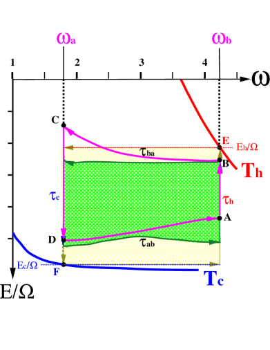
FIG. 1.: The heat engine with $J\neq 0$ in the $\omega~{}$, $E/\Omega$ plane. $T_{h}$ is the hot bath temperature. $\tau_{h}$ is the time allocation when in contact with the hot bath. $T_{c}$ and $\tau_{c}$ represent the temperature and time allocation for the cold bath. $\tau_{ba}$ represents the time allocation for compression (field change from $\omega_{b}$ to $\omega_{a}$) and $\tau_{ab}$ for expansion. The rectangular box which includes point $E$ on the hot isochore where the system is in equilibrium with $T_{h}$, and point $F$ (equilibrium with $T_{c}$ ) on the cold isochore, represents the cycle of maximum work. This cycle spends an infinite amount of time on all branches. The work is the area of the rectangle ${\cal W}_{max}=(\Omega_{b}-\Omega_{a})\cdot(\frac{E_{h}}{\Omega_{b}}-\frac{E_{c}}{\Omega_{a}})$. The optimal power cycle is emphasized by the green shading. The time allocations for this cycle are $\tau_{h}=1.705$,$\tau_{ba}=0.4369$ ,$\tau_{c}=1.76597321$ and $\tau_{ab}=0.4953$. The cycle depicted in purple is characterized by very short time allocations on the adiabats ($\tau_{ba}=\tau_{ab}=0.00025$). The common engine parameters are: $\omega_{a}=1.794$, $\omega_{b}=4.239$ $T_{h}=2.5$, $T_{c}=0.5$, $J=0.6$. $\Gamma_{c}=\Gamma_{h}=1$ with units where $\hbar=1$ and $k_{b}=1$.

The cycle starts at point $\bf A$ where the system is in contact with the hot bath at temperature $T_{h}$. The system accumulates heat for a period $\tau_{h}$ until it reaches point $\bf B$. Point $\bf E$ is the equilibrium point of the scaled energy $E/\Omega$ at the bath temperature $T_{h}$ with external field strength $\omega_{b}$. Adiabatic compression from $\omega_{b}$ to $\omega_{a}$ follows the trajectory from point $\bf B$ to point $\bf C$ for a time duration $\tau_{ba}$ with a constant $\dot{\omega}$. The system is in contact with the cold bath from point $\bf C$ to point $\bf D$ for a time duration $\tau_{c}$. The cold bath equilibrium point, at temperature $T_{c}$ at $\omega_{a}$, is $\bf F$. The cycle becomes closed by a compression stage from point $\bf D$ back to point $\bf A$.

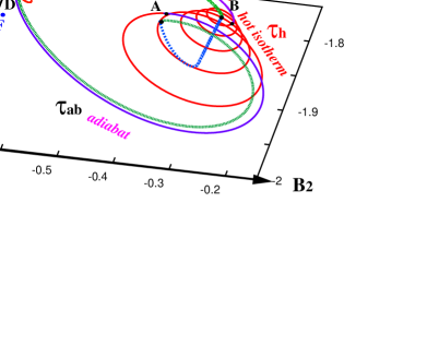
FIG. 2.: The optimal power heat engine cycle corresponding to Fig. 1. The $\bf\hat{B}_{1}$ coordinate represents the individual particle polarization, and the $\bf\hat{B}_{2}$ and $\bf\hat{B}_{3}$ coordinates represent the interparticle correlation. The inner cycle with blue isochores is subject to strong dephasing ($\gamma_{h}=0.15$ and $\gamma_{c}=0.5$).

For long time duration on the adiabats the cycle of operation is restricted to the $\bf\hat{B}_{1}$, $\bf\hat{B}_{2}$ plane. For fast motion on the adiabats the system cannot follow the instantaneous change in the direction of the Hamiltonian rotating on the $\bf\hat{B}_{1}$, $\bf\hat{B}_{2}$ plane. As a result the expectation of the $\bf\hat{B}_{3}$ operator increases starting a precession type motion around the temporary direction of the Hamiltonian ${\bf\hat{H}}=\omega(t){\bf\hat{B}_{1}}+J{\bf\hat{B}_{2}}$. This can be seen clearly in Fig. 2 in the trajectory from point $\bf D$ to point $\bf A$. The precession motion continues on the isochore where the Hamiltonian becomes constant (point $\bf A$ to point $\bf B$). In addition, due to dephasing, the amplitude of the precession motion is damped. Part of the dephasing is caused by the energy equilibration with the bath. When pure dephasing is added the precession motion is damped almost instantly (Cf. fig 2). The motion out of the $\bf\hat{B}_{1}$, $\bf\hat{B}_{2}$ plane causes a bending upward in the adiabats as seen in Fig. 1. This bending causes additional work on the adiabats which is then dissipated on the isochores. This causes a reduction in efficiency from $\eta_{max}=1-\Omega_{a}/\Omega_{b}~{}=0.5581$ which is reached at infinite cycle times to a lower value at maximum power $\eta_{Pmax}=0.495$ ($\eta_{carnot}=0.8$). The cycle of the engine is completely determined by the external control parameters $\omega_{a},\omega_{b},T_{h},T_{c}$, and the time allocations: $\tau_{h},\tau_{c},\tau_{ba},\tau_{ab}$. Independent of the initial condition, the engine settles to a limit cycle after a few revolutions with the preset sequence of isochores and adiabats.

The optimization objective is the power of the engine which is the total work per cycle $\cal W$ divided by the cycle period $\tau$. Work is obtained only on the adiabats and is calculated by integrating the instantaneous power Eq. (3) for the adiabat duration: ${\cal W}_{ba}=\int_{0}^{\tau_{ba}}{\cal P}dt=\int_{0}^{\tau_{ba}}\dot{\omega}\langle{\bf\hat{B}_{1}}\rangle dt$.

The optimization analysis starts by setting the external parameters as the extreme field values $\omega_{b}$, $\omega_{a}$ and the hot and cold bath temperatures at $T_{h}$, $T_{c}$. The performance of the engine therefore will be determined by the time allocated to the different segments. By setting the total cycle time $\tau=\tau_{ba}+\tau_{c}+\tau_{ab}+\tau_{h}$ the optimization is carried out by partitioning the time between the adiabats and isochores. This splits the allocated time between the hot and cold bath isochores, and splits the allocated time between the compression and expansion adiabats.

In the limiting case of no internal coupling $J=0$, the current model is identical to the noted frictionless one [8, 10]. In this frictionless case the optimal power time allocation on the isochores becomes: $\Gamma_{h}\tau_{h}=\Gamma_{c}\tau_{c}$ and zero time allocation on the adiabats. For $J\neq 0$ the time allocations changes considerably. Two limiting cases emerge, the slow limit where most of the cycle time is allocated to the adiabats, and the fast or sudden limit where most of the time is allocated to the isochores.

Due to the precession motion, the cycle operation is noisy. A small change in a parameter can considerably alter the limit cycle and thus the performance of the engine. Additional pure dephasing damps the noise of the engine (Cf. Fig. 2) while the overall performance is only slightly altered.

The global power optimum was sought by both a conjugate gradient method and by a random search scrutinizing local maxima. The optimal power as a function of the total cycle time is shown in Fig. 3 for different $J$ values. It is clear that the power has a clear maximum with respect to the cycle period $\tau$. The optimal value decreases and cycle time increases with increasing $J$. The maximum power output as a function of $J$ is shown in the insert together with the analogous friction case.

Despite the large local fluctuations with respect to time allocations the optimal power performance of the quantum engine shows a remarkable overall similarity to the performance of an engine subject to phenomenological friction as studied in Ref. [10]. One expects friction to oppose the fast motion on the adiabats, therefore the extra power invested has to be independent of the sign of the change in the control field. This means that to the lowest order it has to be proportional to the square of the time derivative i.e. ${\cal P}_{fric}=\sigma^{2}\dot{\omega}^{2}$. The accumulated extra work is then dissipated on the cold isochore. The engine subject to friction shows performance curves and optimal time allocations which are very close to the present first principle quantum model. For this case the origin of lost power is the inability of the ”polarization” vector to follow adiabatically the instantaneous Hamiltonian. The resulting precession motion on the isochores then leads to additional dissipation on the cold isochore. To the lowest order, the additional power should scale as $J^{2}$ which explains the observed linear relation of $J$ with the friction parameter $\sigma$.

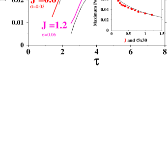
FIG. 3.: Power as a function of cycle time $\tau$ for optimal time allocation on the four branches for three values of the parameter $J$. The underlying dotted lines are the optimized power output of an engine with phenomenological internal friction (in black). A linear relation between $J$ and the friction parameter $\sigma$ fits the data. The insert shows the Maximum power as a function of J (in red) and $\sigma\times 30$.

To conclude, we have found that a quantum heat engine with a working fluid which is not completely controllable by the external field shows performance characteristics which can be mapped into a heat engine subject to phenomenological friction.

This research was supported by the US Navy under contract number N00014-91-J-1498 and the Israel Science Foundation. The authors wish to thank Jeff Gordon for his continuous help.

REFERENCES

- [1]
- [2] F.L. Curzon and B. Ahlborn, Am. J. Phys. 43, 22 (1975).
- [3] P. Salamon, J. D. Nulton, G. Siragusa, T. R. Andersen, A. Limon, Energy, 26 307 (2001).
- [4] R. Kosloff, J. Chem. Phys., 80, 1625–1631 (1984).
- [5] J. Geusic, E. S. du Bois, R. D. Grasse, and H. Scovil, J. App. Phys. 30, 1113 (1959).
- [6] E. Geva and R. Kosloff, J. Chem. Phys., 96, 3054 (1992).
- [7] E. Geva and R. Kosloff, J. Chem. Phys., 97, 4398 (1992).
- [8] T. Feldmann, E. Geva, R. Kosloff and P. Salamon, Am. J. Phys. 64, 485 (1996)
- [9] S. Lloyd, Phys. Rev. A 56 3374 (1997).
- [10] T. Feldmann and R. Kosloff, Phys. Rev. E 61, 4774 (2000)
- [11] E. Geva and R. Kosloff, J. Chem. Phys., 104, 7681 (1996).
- [12] R. Kosloff, E. Geva and J. M. Gordon, Applied Physics, 87, 8093–8097 (2000).
- [13] J. P. Palao, R. Kosloff and J. M. Gordon Phys. Rev. E (2001).
- [14] G. Lindblad, Commun. Math. Phys., 48, 119 (1976).