Polarisation Patterns and Vectorial Defects in Type II Optical Parametric Oscillators

Abstract

Previous studies of lasers and nonlinear resonators have revealed that the polarisation degree of freedom allows for the formation of polarisation patterns and novel localized structures, such as vectorial defects. Type II optical parametric oscillators are characterised by the fact that the down-converted beams are emitted in orthogonal polarisations. In this paper we show the results of the study of pattern and defect formation and dynamics in a Type II degenerate optical parametric oscillator for which the pump field is not resonated in the cavity. We find that traveling waves are the predominant solutions and that the defects are vectorial dislocations which appear at the boundaries of the regions where traveling waves of different phase or wave-vector orientation are formed. A dislocation is defined by two topological charges, one associated with the phase and another with the wave-vector orientation. We also show how to stabilize a single defect in a realistic experimental situation. The effects of phase mismatch of nonlinear interaction are finally considered.

I Introduction

Most studies of pattern [2, 3, 4] and localized structure [5, 6, 7, 8, 9, 10, 11, 12, 13, 14, 15, 16, 17, 18] formation in optical systems consider light with a fixed linear polarisation. However, the vectorial degree of freedom of light, associated with a space- and time-dependent polarisation, leads to a very interesting phenomenology, as previously shown for Kerr cavities [19, 20, 21], sodium vapors [22], lasers [23, 24, 25] and intra-cavity second harmonic generation [26]. This degree of freedom is also relevant from the point of view of information encoding and processing, because it yields a tool for the control of these structures. Optical vortices have been predicted to occur in optical systems such as lasers [27] and they have been experimentally observed in lasers [28] and photo-refractive resonators [13, 29, 30]. More recent theoretical studies revealed the existence of vectorial defects in optical systems [25].

Among optical systems, optical parametric oscillators (OPO’s) have been the object of intense theoretical study in recent years, which has revealed the existence of patterns [31, 32, 33, 34, 35, 36, 37, 38, 39, 40, 41, 42] and localized structures [11, 14, 15, 18, 43, 44, 45, 46]; few examples of defect dynamics have also been published [18, 39, 47]. Finally, experimental results on transverse pattern formation have been recently presented [48, 49]. An OPO consists of a ring (or Fabry-Perot) resonator containing a nonlinear quadratic medium, which performs a parametric down-conversion of an injected laser beam (optical pump) at frequency $\omega_{p}$. Two new fields are generated in the crystal, the signal and the idler, at frequencies $\omega_{s},\omega_{i}$ respectively, such that $\omega_{p}=\omega_{s}+\omega_{i}$, the last relation indicating the conservation of photon energy. The nonlinear interaction also requires photon momentum to be conserved, i.e. the phase-matching condition $k_{p}-k_{s}-k_{i}=0$, which is usually obtained by exploiting polarized beams and crystal birefringence. This effect often implies that a transverse walk-off between the different polarisation components may occur. The consequences of walk-off have also been considered and convective instabilities and noise-sustained patterns found [40, 41, 46, 50, 51]. Most of these theoretical studies have been performed in the context of a scalar approximation, which is valid for the so called Type I OPO’s; in the Type I interaction the signal and idler fields have the same polarisation, orthogonal to the pump beam. However, there are not many studies involving Type II OPO’s where the polarisation degree of freedom is taken into account. In refs. [32, 35, 36, 39] the model equations can be valid for an OPO that is non degenerate either in polarisation or in frequency; however the intrinsic physical difference between the two cases was not made evident. In refs. [47] and [52] the polarisation non-degenerate case and the polarisation and frequency non-degenerate case have been considered and the role of the walk-off explored. Finally the case of polarisation coupling, due to cavity birefringence and/or dichroism has been analysed for the case of an OPO, showing Bloch walls formation [53]; these structures were later found also for second harmonic generation [54].

In this paper we will focus our attention on the polarisation pattern and vectorial defect formation in a Type II, frequency degenerate OPO. In particular we will consider the case in which the pump is not resonated in the cavity and can be eliminated from the dynamics by means of a multiple scale approximation. This simplification has also been made in order to take into account the effects of phase mismatch, which has been only partly studied in connection with Type I OPO’s [34]. In fact, the conservation of the photon momentum need not to be exact for down conversion to occur, the conversion efficiency being lower if $k_{p}-k_{s}-k_{i}\neq 0$.

The paper is organized as follows. In section II we present the equations which model the Type II OPO and some exact, stable solutions, which are combinations of traveling waves (TW’s). Due to the vectorial nature of the field these solutions represent spatial polarisation patterns. We also show that these TW’s are spontaneously formed starting from a random perturbation of the trivial steady-state, that is represented by the field below the threshold of signal and idler generation. In section III we show that, on a background made of TW’s, vectorial defects are spontaneously generated. The defects are classified as vectorial dislocations by comparing the quantities characteristic of a dislocation of a complex field with those of the defects obtained in the dynamical system. The dynamics of defects is also studied in this section. The stabilization of a single defect is then presented in section IV. The discussion of the effects due to the presence of the phase mismatch is given in section V and the conclusions presented in section VI. In Appendix I we derive the basic equations in which our study is based, and in Appendix II we derive the corresponding amplitude equation (a Swift-Hohenberg equation) for the instability leading to frequency-converted light generation in our model.

II Equations and background solutions

We considered a model for a Type II OPO, for which the pump is not resonated in the cavity and in which some mismatch among the interacting waves is allowed. Previous studies of pattern formation, except ref. [34], neglected mismatch; however real devices are likely to present a residual mismatch due to the selection mechanism of the signal and idler frequencies (see [55] for details). Since the Type II configuration means that the signal and the idler are orthogonally polarized fields we will use the notation $A_{x},A_{y}$ to denote them. The starting point is the slowly varying envelope approximation propagation equations for a Type II interaction which include the mismatch (see for example [56]). By following the procedure outlined in Appendix I, we obtain the evolution equations for the cavity fields:

$$\partial_{t}A_{x} = \gamma_{x}[-(1+i\Delta)A_{x}+\mu A_{y}^{*}+\sigma|A_{y}|^{2}A_{x}]+ia_{x}\nabla^{2}A_{x}$$ (1)

$$\partial_{t}A_{y} = \gamma_{y}[-(1+i\Delta)A_{y}+\mu A_{x}^{*}+\sigma|A_{x}|^{2}A_{y}]+ia_{y}\nabla^{2}A_{y}$$ (2)

where $\gamma_{x},\gamma_{y}$ are the decay rates of the signal and idler in the cavity, $\Delta$ the cavity detuning, $a_{x},a_{y}$ the diffraction coefficients. Note that the detunings of the two fields are made equal to a common value $\Delta$ [57] by choosing the temporal reference frame such that stationary homogeneous states do not have free rotating phases. The other terms which appear in these coupled equations are respectively:

a) a linear parametric coupling with coefficient

$$\mu=E_{0}exp(\frac{i\Delta kL}{2})\frac{sin(\Delta kL/2)}{\Delta kL/2}$$ (3)

where $E_{0}$ is the injected pump field, $\Delta k$ the photon momentum mismatch and $L$ the crystal length [58];

b) a cubic nonlinear coupling with coefficient

$$\sigma=\frac{2}{\Delta k^{2}L^{2}}[(cos(\Delta kL)-1)+i(sin(\Delta kL)-\Delta kL)]$$ (4)

At perfect phase-matching $\mu=E_{0},\sigma=-1$ ; otherwise the coefficients are complex numbers; their real, imaginary parts are shown in fig. 1 for $E_{0}=1.5$. Similar coefficients were also found for a Type I, singly resonant frequency degenerate OPO, by Longhi in ref. [34], with the same type of analysis. Note that the lasing of an OPO requires $|\Delta k|<\pi/L$ because the parametric gain outside this range is too small and the device tends to ”jump” to another pair of signal-idler frequencies which satisfy this condition [55]. Finally note that all coefficients can become dimensionless as soon as appropriate time, space and field amplitude scaling are performed.

Equations (1,2) have exact traveling wave solutions of the same type as those found in ref. [36]:

$$\left(\begin{array}[]{c}A_{x}\\ A_{y}^{*}\end{array}\right)=\sqrt{C}e^{i(\omega t+{\bf k}\cdot{\bf r})}\left(\begin{array}[]{c}e^{i\phi_{0}}\\ e^{-i(\alpha-\phi_{0})}\end{array}\right)$$ (5)

where $\phi_{0}$ is an arbitrary phase, while the intensity $C$ and the phase difference $\alpha$ between the signal and the idler are given by

$$C=\frac{1}{|\sigma|^{2}}\left[\sigma^{\prime}+\sigma^{\prime\prime}\tilde{\Delta}\pm\sqrt{|\mu|^{2}|\sigma|^{2}-(\sigma^{\prime\prime}-\sigma^{\prime}\tilde{\Delta})^{2}}\right]$$ (6)

$$cos\alpha=\frac{1}{|\mu|^{2}}[\mu^{\prime}(1-\sigma^{\prime}C)+\mu^{\prime\prime}(\tilde{\Delta}-\sigma^{\prime\prime}C)]$$ (7)

where $\sigma^{\prime}=Re(\sigma),\sigma^{\prime\prime}=Im(\sigma)$, $\mu^{\prime}=Re(\mu),\mu^{\prime\prime}=Im(\mu)$ and $\tilde{\Delta}=\Delta+|{\bf k}|^{2}(\gamma_{x}a_{x}+\gamma_{y}a_{y})/(\gamma_{x}+\gamma_{y})$ is an effective detuning parameter. The TW intensity $C$ and the phase difference $\alpha$ are shown in fig. 2 for $E_{0}=1.5$.

The frequency shift $\omega$ is given by:

$$\omega=\frac{\gamma_{x}\gamma_{y}}{\gamma_{x}+\gamma_{y}}[(a_{y}-a_{x})|{\bf k}|^{2}]$$ (8)

This quantity can be zero if the diffraction coefficients are equal for the signal and the idler. Hereafter we will consider only the case of frequency degenerate OPO, i.e. when the frequency of the signal and idler are the same; this also implies that $\gamma_{x}\simeq\gamma_{y}$ (without loss of generality we set $\gamma_{x}=\gamma_{y}=1$ in our simulations, thus scaling time with the cavity lifetime). The condition $a_{x}=a_{y}=a$ can be exactly obtained for example by introducing compensating prisms in the cavity, as suggested in Appendix I. Strictly speaking if $\omega=0$ the solutions (5) are not traveling waves but rather standing phase waves; however, we will generally refer to them as TW. It is important to note that considering the case $\omega=0$ is not restrictive in the sense that all features observed for this case survive also for $\omega\neq 0$, at least when a uniform pump and periodic boundary conditions are used. We checked this by integrating eqs. (1,2) also for $a_{x}\neq a_{y}$; the main difference is that phase waves travel. Under the hypothesis made in this paragraph the effective detuning simply reads $\tilde{\Delta}=\Delta+a|{\bf k}|^{2}$.

TW solutions (5) exist for $|\mu|^{2}>1+\tilde{\Delta}^{2}=|\mu_{c}|^{2}$ if $\sigma^{\prime}+\sigma^{\prime\prime}\tilde{\Delta}<0$; in this case only the solution with the plus sign is acceptable in eq. (6). If $\sigma^{\prime}+\sigma^{\prime\prime}\tilde{\Delta}>0$ solutions exist for $|\mu|^{2}>|\mu_{c}|^{2}-\frac{1}{|\sigma|^{2}}(\sigma^{\prime}+\sigma^{\prime\prime}\tilde{\Delta})$ and there is bistability up to $\mu_{c}$ among the solutions obtained by taking the plus and minus signs. However, when no mismatch is present ($\Delta k=0$), given that $\sigma^{\prime}<0$, no bistability regime exists and TW are found only for $|\mu|^{2}>|\mu_{c}|^{2}=1$. Note that if no mismatch is present the solutions also satisfy $\alpha=0$ and therefore $A_{x}=A_{y}^{*}$. Hereafter we will consider only the case of perfect phase-matching and leave the observations about the effects of mismatch to section V.

A physical interpretation of the exact solutions can be given in terms of spatial polarisation patterns. In fact, under the assumptions made, the Stokes parameters [59]

$$S_{0} = |A_{x}|^{2}+|A_{y}|^{2}$$ (9)

$$S_{1} = |A_{x}|^{2}-|A_{y}|^{2}$$ (10)

$$S_{2} = A_{x}A_{y}^{*}+A_{x}^{*}A_{y}$$ (11)

$$S_{3} = i(A_{x}A_{y}^{*}-A_{x}^{*}A_{y})$$ (12)

associated with the TW’s at frequency $\omega_{s}=\omega_{i}=\omega_{p}/2$ can be simply calculated as

$$S_{0}=2C,\;\;\;\;S_{1}=0,\;\;\;\;S_{2}=2\;\;C\;cos(2{\bf k_{c}}\cdot{\bf r}-\alpha),\;\;\;\;S_{3}=2\;C\;sin(-2{\bf k_{c}}\cdot{\bf r}+\alpha)$$ (13)

These equations mean that the coupled-TW solution $(A_{x},A_{y})$ represents an elliptically polarized field with a two-valued spatially periodic azimuth ($\theta=tan^{-1}(S_{2}/S_{1})/2$) and with a spatially periodic ellipticity parameter $\eta({\bf r})=\alpha/2-{\bf k_{c}}\cdot{\bf r}$. In particular, in the direction of the wave-vector ${\bf k_{c}}$ the polarisation changes from linear (with $\theta=\pi/4$), to right circular, to linear (with $\theta=-\pi/4$), then to left circular and back again to linear (with $\theta=\pi/4$) with a spatial period $\lambda_{c}/2=\pi/k_{c}$ (see fig. 3).

Other stable solutions can be found as combinations of the basic TW solutions (5) as shown in ref. [35] for a triply resonant, non-degenerate OPO. They can be generally written as:

$$\left(\begin{array}[]{c}A_{x}\\ A_{y}^{*}\end{array}\right)=(f_{1}exp(ik_{c}x)+f_{2}exp(ik_{c}y)+f_{3}exp(-ik_{c}x)+f_{4}exp(-ik_{c}y))\left(\begin{array}[]{c}1\\ 1\end{array}\right)$$ (14)

The coefficients $f_{k}$ determine the kind of solution; for example the TW is $(f_{1},f_{2},f_{3},f_{4})=(\sqrt{C},0,0,0)$ and the standing rolls are $(\sqrt{C},0,\sqrt{C},0)$. An interesting solution for this case is that of the alternating rolls $(f_{1},f_{2},f_{3},f_{4})=(\sqrt{C},i\sqrt{C},\sqrt{C},i\sqrt{C})$ i.e.:

$$\left(\begin{array}[]{c}A_{x}\\ A_{y}^{*}\end{array}\right)=2\sqrt{C}(cos(k_{c}x)+i\;cos(k_{c}y))\left(\begin{array}[]{c}1\\ 1\end{array}\right)$$ (15)

that gives rise to a square intensity pattern. We found that this structure is stable with periodic boundary conditions, but it deforms and disappears as soon as other, more realistic, boundary conditions are applied. We show in fig. 4 the square array with periodic boundary conditions after an evolution of $t=500$ time units; no appreciable change of the initial condition (15) has been observed.

The equations also have a trivial steady-state solution $A_{x}=A_{y}=0$, that represents the non lasing state of the OPO and whose stability analysis is similar to that performed in refs. [31, 32, 36]. Briefly, $A_{x}=A_{y}=0$ becomes unstable for $|\mu|>1$ if $\Delta<0$ and for $\mu>\sqrt{1+\Delta^{2}}$ if $\Delta>0$. For $\Delta>0$ the trivial solution becomes unstable for homogeneous perturbations ($k_{c}=0$) and no pattern or structure is expected to be spontaneously formed. In numerical simulation we observed the transition to a final, stable, homogeneous state of intensity $C$, preceded by a transient regime where domain walls form but soon disappear [18]. For $\Delta<0$ the most unstable modes are TW with a critical wave-vector $|{\bf k_{c}}|^{2}=-\Delta/a$, i.e. such that the equivalent detuning $\tilde{\Delta}$ is zero. Note that the most unstable modes are also exact TW solutions of eqs. (1,2). Although stability of such TW’s was not studied, numerical solutions give evidence that they are stable and moreover that they are spontaneously formed starting from a random perturbation of the trivial steady-state when the pump amplitude is above the threshold of the parametric interaction. Then, the spontaneously selected TW’s have wave-vector modulus $|{\bf k_{c}}|=k_{c}=\sqrt{-\Delta/a}$ but a random orientation or phase in different region of space; this causes the occurrence of defects in the patterns as will be shown below. Hereafter we will treat only the case of polarization pattern formation, i.e. $\Delta<0$.

If the pump amplitude is weakly above the threshold ($5\%$) two different final situations can be found starting from a random perturbation of the trivial steady-state under periodic boundary conditions. In the first, all defects initially formed tend to annihilate each other and the final state is a single TW of random orientation, whose wave-vector is exactly $k_{c}$. As in the case of non-degenerate OPO’s [36] no intensity patterns appear but only phase stripe patterns, which correspond to the polarisation patterns described by eqs. (5) and (13). In another case, for the same pump amplitude but with other initial random conditions, ordered structures of defects may form as shown in fig. 5. By looking at the real and imaginary parts of the field $A_{x}$ it is clear that these defects are found along the fronts which separate regions where TW’s with the same wave-vector but with different phase have been selected. From the figure it is also clear that these defects appear on a background of TW solutions, at those points where the stripes do not match.

Defects also appear spontaneously with pump amplitudes well above threshold ($50\%$); in this case the positions of the defects are not ordered, as shown for example in fig. 6 a) and b). Defects always appear in both orthogonal polarisation components (i.e. the signal and the idler simultaneously) and therefore they can be classified as vectorial, since the two components of the vector field $(A_{x},A_{y})$ are zero at the same point in space. In fig. 6 c) and d) the phase of the polarisation components is also presented; note that it is not defined at the points where the amplitude goes to zero. Then, such objects require a topological classification that is furnished in the next section. Finally note that setting $a_{x}\neq a_{y}$ or $\gamma_{x}\neq\gamma_{y}$ does not alter the basic features observed; defects persist and are advected by the phase waves, which now travel as previously described. This has been cheked by running the same simulation (i.e. that of fig. 5) with and without equal coefficients.

It is always useful to have in mind the general characteristics of the instability of the zero state in our OPO model, in order to relate it to other pattern forming systems. In our case, the instability for $\Delta<0$ is at a non vanishing wavenumber $k_{c}$, so that a Swift-Hohenberg equation for the complex envelope of the unstable modes is the appropriate amplitude-equation description close to threshold. For the case $a_{x}=a_{y}$, this Swift-Hohenberg equation has real coefficients. This equation is derived from our basic equations (1,2) in Appendix II.

III Defect classification, formation and dynamics

In this section we analyse the formation and dynamics of defects, in Type II OPO’s. The existence of defects in a Type I non-degenerate triply resonant OPO was pointed out in ref. [39] where the dynamics of an advected defect pair was also reported. Here, we present a detailed study of the defects which spontaneously appear in the Type II frequency degenerate OPO. The analysis includes: a) the classification of the defect type, showing that these defects are dislocations of the TW pattern; b) the formation process under several different conditions and regimes and c) the trapping and stabilization of a single defect.

A dislocation of a scalar complex field $A(r,\theta)$, $(r,\theta)$ being spatial polar coordinates, can be defined as a configuration which can be deformed continuously (in a neibourhood of a point ${\bf r_{0}}$, which is then identified as the core of the dislocation and it is taken as the origin of the polar coordinates) into the following function:

$$A(r,\theta)=R(r)\;exp(i(\theta+kr\;cos\theta))=R(r)\;exp(i\phi)$$ (16)

The function $R(r)$ is real and depends on the radial coordinate such that $R(0)=0$. This condition is necessary because the phase $\phi$ of the field is not defined in the origin of coordinates. In fig. 7 a) we show the real part of $A$ from which we can observe that the defect is found at the point where the stripes of the background, whose wave-vector far from the defect is $k$, do not match. The phase $\phi$ is shown in fig. 7 b); the defect is centered at the point ${\bf r_{0}}=0$, around which the phase changes by $2\pi$. The topological charge associated with the phase change is defined by the integral of the phase gradient on a closed contour surrounding the point ${\bf r_{0}}$

$$n_{0}=\frac{1}{2\pi}\oint_{{\bf r_{0}}}\nabla\phi\cdot d{\bf r}=1$$ (17)

Note that there exists also another dislocation obtained by setting $\theta\rightarrow-\theta$ for which the topological charge $n_{0}$ is equal to $-1$. However the most interesting feature of a dislocation is that it is characterised by another topological charge. This is associated with the function

$$\psi(x,y)=tan^{-1}\left(\frac{(\nabla\phi)_{y}}{(\nabla\phi)_{x}}\right)$$ (18)

where the indices $x,y$ of the term on the right hand side refer to the vector components. This function, which defines the orientation angle of the wave-vector ${\bf k}$, is shown in fig. 7 c) for the field $A$ defined by eq. (16). Note that there are two points where $\psi$ is not defined: one is located at the point ${\bf r_{0}}$, corresponding to the point of zero amplitude; the second is at another point ${\bf r_{1}}$ where $|{\bf r_{1}}-{\bf r_{0}}|=k^{-1}$. Then, the topological charges associated with $\psi$ are:

$$m_{0}=\frac{1}{2\pi}\oint_{{\bf r_{0}}}\nabla\psi\cdot d{\bf r}=1$$ (19)

where the integration contour surrounds the point ${\bf r_{0}}$ but leaves outside the point ${\bf r_{1}}$ and

$$m_{1}=\frac{1}{2\pi}\oint_{{\bf r_{1}}}\nabla\psi\cdot d{\bf r}=-1$$ (20)

where the integration contour surrounds the point ${\bf r_{1}}$ but leaves outside the point ${\bf r_{0}}$. Note that there is not a zero in the amplitude $R$ at the point ${\bf r_{1}}$.

We now turn our attention back to the Type II OPO and compare the defects which are found in the numerical solutions of eqs. (1,2) with the dislocation just defined. In this section, to better compare numerical and theoretical results only periodic boundary conditions and homogeneous pump beams are considered; more realistic conditions will be explored in section (IV) when stabilization of a dislocation is considered.

The randomly generated defects of figures 5 and 6 are dislocations on a background of TW’s, although in the second case it is difficult to recognize the background solutions since the defects are dense in the integration window. However a fingerprint of TW is found also for the data of fig. 6 by observing the far field in fig. 8. There, a ring of modes of radius $k_{c}$ is clearly observable, a clear indication that the background is made mostly of TW solutions of different orientation but the same wave-number $k_{c}$. The dislocations can be also clearly identified when the quantities $\psi_{x}$ and $\psi_{y}$ (defined again through eq. (18) where the phases are those of $A_{x},A_{y}$) are calculated for the same data of fig. 6. The result is presented in figures 9 a) and b) where a contour plot of $|A_{x}|,|A_{y}|$ taken at a low intensity level to indicate the locations of the zeros of the field, is superimposed on the grey-scale coded images of the functions $\psi_{x}$ and $\psi_{y}$. From fig. 9 we note that in this static condition “chains” of defects of the functions $\psi_{x,y}$ are formed. Two zeros of the amplitude (defects of charges $n_{0},m_{0}$) are in fact connected by the relative pair of defects of the functions $\psi_{x,y}$ at the second point (defects of charge $m_{1}$). This stems from the fact that the phase difference between $A_{x}$ and $A_{y}$ is zero (when there is no mismatch) and thus $A_{x}=A_{y}^{*}$.

Regarding the dynamics [60] of the spontaneously generated defects, we observe that they appear at the early stage of the process. Some of them are annihilated within a few thousand cavity lifetime units. After this stage we cannot observe any annihilation, up to 100000 cavity lifetime units. The initial number of dislocations and their positions change with different initial conditions. The statistical distribution of the final number of defects, by changing initial conditions, is shown in fig. 10; observe that a Gaussian fit is actually very good. We note that the defect density never reaches that of the square pattern (eq. (15)) with critical wave-vector $k_{c}$. After the initial formation stage, we observe in our runs that defects have a slow, random motion. This regime is mostly dominated by the attraction of pairs of defects of opposite charges $n_{0}=\pm 1$. For longer times the motion tends to stop and an equilibrium condition is reached. Although no detailed statistical study has been conducted we also note, by inspection of fig. 9, that there seems to exist a characteristic length of separation between the defects, which is an indication that an equilibrium is likely to be reached.

To better study defect interaction we use (16) as an initial condition and integrate eqs. (1,2). Due to the periodic boundary conditions a pair of defects is generated, as shown in fig. 11 a). These correspond to two dislocations in the real part of each field (fig. 11 b)), two phase singularities with opposite topological charge (fig. 11 c)) and two pairs of defects associated with the quantity $\psi_{x}$ (fig. 11 d)). At the initial stage the zeros of the amplitude, which have opposite $n_{0}$ charge, attract each other; later, when the $\psi_{x}$ defects (which have the same charge $m_{0}=1$) get closer, this attraction is stopped and an equilibrium position is found [60]. This paired structure is stable at least up to the time explored by numerical solutions.

In general, the detailed behavior of defects dynamics is governed both by local, phase curvature effects and by defect-defect interactions. The range of these interactions depends on the parameters of the system, which determine the spatial extent of the defect. For example if we make the detuning more negative (e.g. $\Delta_{x}=\Delta_{y}=-1$ and $a_{x}=a_{y}=1$) two defects displaced parallel to the background wavefronts either annihilate, if close enough, or repel each other, if further away.

Figure 12 also shows a pair of defects (same parameter values as in Figure 11 but different initial displacement) undergoing motion; the background has a wave-vector of $2k_{c}$ and it is stable when the system is pumped far above threshold. When their separation is small enough, the defects briefly rotate around each other before continuing their transverse motion. As a consequence of this motion and the periodic boundary conditions, the defects collide and annihilate shortly afterwards (not shown).

Figure 13 shows another interesting example. Two defects approach each other while the background phase wave undergoes a zig-zag instability [61]. When they meet they form a bound pair which follows the local curvature of the background phase fronts, changing direction as the slow phase dynamics alters this curvature. The bound defect pair is stable for the duration of the simulation (115000 cavity lifetimes). It also exists for lower pump powers, down to at least five percent above threshold. On the other hand, at slightly higher pump powers than that used in Figure 13, the structure destabilises: after a short time the defect pair rotates slightly before annihilating.

The previous examples show that long–lived defect interactions are important features of the dynamics of Type II OPO’s. This fact is in agreement with instances of long term survival of many defects generated by random initial conditions (e.g. Fig. 6) and is clearly different from vortex dynamics observed, for example, in complex Ginzburg-Landau models [62].

Close to threshold, it is possible to study the behavior of the Type II OPO dislocations by means of amplitude equations. These are derived in Appendix II where comparisons are made with simulations of the full model.

IV Trapping of isolated dislocations

We know that periodic boundary conditions always require the total topological charge within the domain to be zero. In this section, we take into account that the pump amplitude $E_{0}$ actually has a spatial dependence and periodic boundary conditions are not applicable. If a spatial Gaussian or super-Gaussian distribution is used for the parametric gain factor $\mu$ (eq. (3)), the spontaneously generated defects often tend to move to the region where the field is zero. The trapping of single defects necessary for their experimental observation as single entities is then an interesting issue.

We tried, successfully, to isolate a single defect in a more realistic pump beam, by using, as an initial condition for one of the fields, a doughnut mode. This idea follows the experimental results of induced dislocation formation in quadratic nonlinear interactions [63]. Note that no cavity was used in those experiments and the defect was maintained by forcing a doughnut mode in the field at the crystal input. Here the dislocation is ”written” at the beginning but, after that, no injection is required since the cavity provides the necessary feedback to sustain the structure. The resulting, stable trapped defect is shown in fig. 14. The spiral wave in the phase field spins when $a_{x}\neq a_{y}$, otherwise it is stationary after the initial formation stage. Note that in order to trap the defect the beam size must be kept smaller than the wavelength of the most unstable TW $\lambda_{c}=2\pi/k_{c}$ otherwise more defects are induced or the initial defect is dragged outside the beam. The creation of other defects is due to the tendency of the system to generate pairs. If the system size is comparable with the critical wavelength, the paired defect will appear inside the pumping region and will destabilize the original defect. If the size is smaller the second defect will be generated outside the pumping region and therefore will not influence the dynamics of the trapped defect (fig 14 c)). The amplitude profiles of the fields of this single defect are shown in fig. 15.

This way of generating the defects is also useful for understanding the mechanism of their formation. The presence of a defect in one field, say $A_{x}$, induces a defect of opposite charge $n_{0}$ in the other because of the parametric coupling. In fact if $A_{x}\simeq 0$ at $t=0$ the term which dominates the dynamics of $A_{y}$ in the initial regime is the largest linear one, i.e. $\mu A_{x}^{*}$. Hence, $A_{y}$ is forced by the complex conjugate of $A_{x}$ and a defect of opposite charge is formed. Eventually the other terms of eqs. (1,2) become significant: the real part of the cubic term provides the saturation which stabilizes the solution and nonlinear phase modulations appear if mismatch is present, due to its imaginary part.

If we initialise a defect with topological charge $n_{0}=\pm 2$ using the technique described above, we observe that it breaks up into two defects of charge $n_{0}=\pm 1$.

Since the generation of such defects has been seeded externally, the question arises whether it is possible to obtain defects for positive detunings. In spite of the absence of stable traveling–wave solutions, single vortices can be trapped by using the same seeding technique.

We also observe that walk-off removes all structures from the pumping region and a single TW is selected asymptotically. However, it is interesting to note that in the transient regime dislocations are formed. They appear at the front which divides two regions where stripes with different wave-vector modulus are selected. The difference in the wave-vectors is due to the walk-off, as shown in ref. [47].

Finally, we estimate the threshold for the observation of this isolated dislocation in an OPO. Considering data for $KTiOPO_{4}$ [64]: $\chi=7.33\,pm/V,n_{0}=1.8$ at $\lambda_{0}=1.064\mu m$, and by using the definition of the effective coupling paramater defined in Appendix I ($\alpha$) and considering a nonlinear crystal length of $1cm$, a mirror transmittivity $10^{-2}$, the input field at threshold (E=1) can be evaluated as $E_{IN,0}\simeq 2\,10^{4}\,V/m$ that yields an intensity $I=n_{0}/2\,(\mu_{0}/\epsilon_{0})^{1/2}|E_{IN,0}|^{2}\simeq 1MW/m^{2}$ ($\mu_{0},\epsilon_{0}$ are respectively the vacuum magnetic permeability and electric permittivity constants). The super-Gaussian beam used in the simulation has a beam diameter of about 10 normalized units; a spatial normalized unit corresponds, for the diffraction coefficient of the simulation to about $0.195mm$; hence the CW threshold power is about $0.95W$. The physical cavity decay rates $\gamma_{x,y}$ are about $0.17GHz$ while the cavity detuning is $34MHz$. All these data are compatible with an experimental realization.

V Mismatch effects

This section is dedicated to the study of the effects of mismatch ($\Delta k\neq 0$) between the fields in the OPO. As previously noted, in real devices it is often possible that the selection rules of the oscillation frequencies force the OPO to emit radiation with a slight mismatch [55].

The effects of the mismatch, predicted by the analysis of section II, are the following: a) an increase in the threshold for signal generation (i.e. the instability, see eq. (3)); b) a spatial shift of the iso-polarisation lines for the exact TW solutions. The latter effect is due to the appearance of the phase shift $\alpha\neq 0$ (see eq. (5)) between polarisation components; this stems from the imaginary parts of the coefficients $\mu$ and $\sigma$, the contribution of the latter being a nonlinear phase modulation due to the $\chi^{(2)}:\chi^{(2)}$ cascading effect [65].

For the case of the spontaneous generation of defects we have been able to determine that the phase shift $\alpha$ is non zero in the regions where the background solution dominates. The numerically found value is very close to the value predicted by eq. (7). However, approaching the zeros of the amplitude the phase difference also tends to zero although the phase of the fields is not strictly defined at the defects. In practice the zeros of the spatial function $\alpha(x,y)$ are located exactly at the positions of the field defects. This behavior can be explained as follows: close to the defects the cubic terms tend to zero; in particular the term proportional to the imaginary part of $\sigma$ (i.e. the Kerr-like phase modulation term) is the first that can be neglected. Although $\mu=|\mu|exp(i\beta)$ is complex, by an appropriate re-definition of the variables as $\tilde{A_{j}}=A_{j}exp(i\beta/2)$ $j=1,2$ we can obtain a set of equations for $\tilde{A_{j}}$ where the parametric gain is purely real ($\mu^{\prime\prime}=0$). Thus, we reduce the problem to the case where no mismatch is present (see eq. (7)) and therefore $\alpha\rightarrow 0$.

The final number of spontaneously generated dislocations seems also to be affected by the phase mismatch. We note that this number decreases by changing the mismatch from negative to positive values, keeping all the other parameters fixed. In particular it seems that positive values of the mismatch encourage the annihilation of the pairs of dislocations. This has been verified by numerical integrations with the same parameters and initial conditions as fig. 11 but with non zero mismatch. For $\Delta k>0$ we observed that the pair is annihilated, while for $\Delta k<0$ the pair reaches a stable configuration. A possible cause of this asymmetry is the phase modulation $\alpha$ introduced by the mismatch, which changes sign according to the sign of the mismatch (see fig. 2).

The effect of phase mismatch on the trapped defect is to destabilise it, by generating asymmetries in the fields for both positive and negative values of $\Delta k$.

VI Conclusions

In conclusion we have studied the polarisation pattern and vectorial defect formation in a Type II frequency degenerate optical parametric oscillator.

We found that the preferred solutions, those that are selected out of an initial perturbation of the zero state, are conjugate traveling waves in the two components of the polarisation. A spatial polarisation pattern is then formed: the state of polarisation changes along the spatial coordinate parallel to the selected wave-vector ${\bf k_{c}}$ with period equal to $\lambda_{c}/2=\pi/k_{c}$. In particular the state of polarisation changes along the meridian of the Poincare sphere which passes through the linearly polarized states of azimuth $\theta=\pm\pi/4$ if $\Delta k=0$. The magnitude of the wave-vector of the selected solution is fixed by the parameters and has a single random orientation close to threshold and multiple random orientations far from threshold. Combinations of traveling waves, that form square patterns are also stable solutions and, close to the threshold of the instability, ordered arrays of defects can form spontaneously.

Such defects are isolated zeros of the two linear components of the polarisation, i.e. they are vectorial defects. They are dislocations which form in spatial positions where the background solutions (traveling waves) do not match spatially. Two different kinds of topological charge must be defined: one kind of charge is associated with the phase and two charges with the director angle of the field wave-vector. The first charge, located at the point where the amplitude goes to zero, can be $\pm 1$ and is always opposite in the two polarisation components. The charge associated with the wave-vector is always $+1$ at the point where the amplitude is zero and $-1$ at the paired point, where the amplitude is not zero. The polarisation components are totally correlated; in fact all defects, both in the phase and wave-vector fields, have a corresponding defect in the other polarisation component. In this way the defects form chains in which the separation among defects seems to have a typical size, which is of the order of the background wavelength.

The trapping of an isolated defect has also been demonstrated. This is accomplished by keeping the size of the pump beam smaller than the critical wavelength of the preferred traveling wave such that a second defect cannot be created inside the pump beam but rather lies outside and does not influence the dynamics.

Finally, we have addressed the effects which may arise when the nonlinear interaction is slightly phase mismatched, i.e. the increase in the threshold of signal generation, and the linear and nonlinear phase shifts among the polarisations, the latter due to the cascading effect. Numerical results showed that a positive mismatch can favor the annihilation of dislocations.

Possible applications of defects can be foreseen in the field of particle and atom trapping [66].

VII Appendix I

In this appendix we derive the dynamical equations for a cw Type-II OPO in the presence of diffraction. We start from the amplitude equations for the pump, signal and idler fields in the crystal [56]

$$\partial_{z}E_{0}+\frac{n_{0}}{c}\,\,\,\partial_{t}E_{0} = \frac{i}{2k_{0}}\nabla^{2}E_{0}-\frac{4\pi\Omega_{0}\chi}{n_{0}c}\,\,\,E_{x}E_{y}\,\,\,e^{-i\Delta kz}$$ (21)

$$\partial_{z}E_{x}+\frac{n_{x}}{c}\,\,\,\partial_{t}E_{x} = \frac{i}{2k_{x}}\nabla^{2}E_{x}+\frac{4\pi\Omega_{x}\chi}{n_{x}c}\,\,\,E_{0}E_{y}^{*}\,\,\,e^{i\Delta kz}$$ (22)

$$\partial_{z}E_{y}+\frac{n_{y}}{c}\,\,\,\partial_{t}E_{y} = \frac{i}{2k_{y}}\nabla^{2}E_{y}+\frac{4\pi\Omega_{y}\chi}{n_{y}c}\,\,\,E_{0}E_{x}^{*}\,\,\,e^{i\Delta kz}.$$ (23)

where $E_{0},E_{x},E_{y}$ are the slowly varying amplitudes of pump, signal and idler respectively, $\Omega_{0}=\Omega_{x}+\Omega_{y}$ is the frequency constraint on the OPO, $k_{i}=n_{i}\Omega_{i}/c$ are the wave-numbers, $\Delta k=k_{0}-k_{x}-k_{y}$ is the phase mismatch, $\chi$ is the second order susceptibility of the crystal, and $c$ is the speed of light. We treat here the perfectly matched case ($\Delta k=0$) in order to focus on the form of the diffraction coefficients of the final equations. The phase matching condition implies that once the three frequencies and two refractive indices are given, then the third refractive index is determined. For example for $n_{0}$ we have

$$n_{0}=\frac{n_{x}\Omega_{x}+n_{y}\Omega_{y}}{\Omega_{x}+\Omega_{y}}\;\;\;\;\;\;\;\;\;\;\;\;\;\;\;\;\;\;\;n_{0}=\frac{n_{x}+n_{y}}{2}$$ (24)

where the second equation is valid at frequency degeneracy. It is also useful to introduce $\Omega_{x}=\mu\Omega_{0}$, $\Omega_{y}=\nu\Omega_{0}$ with $\mu+\nu=1$ and the effective coupling parameter $\alpha=4\pi\Omega_{0}\chi/(nc)$ to obtain

$$\partial_{z}E_{0}+\frac{n_{0}}{c}\,\,\,\partial_{t}E_{0} = \frac{i}{2k_{0}}\nabla^{2}E_{0}-\alpha E_{x}E_{y}$$ (25)

$$\partial_{z}E_{x}+\frac{n_{x}}{c}\,\,\,\partial_{t}E_{x} = \frac{i}{2k_{x}}\nabla^{2}E_{x}+\mu\alpha E_{0}E_{y}^{*}$$ (26)

$$\partial_{z}E_{y}+\frac{n_{y}}{c}\,\,\,\partial_{t}E_{y} = \frac{i}{2k_{y}}\nabla^{2}E_{y}+\nu\alpha E_{0}E_{x}^{*}.$$ (27)

All these equations describing the fields in the crystal have a similar form of the kind

$$\partial_{z}E_{i}+\frac{n_{i}}{c}\partial_{t}E_{i}=id_{i}\nabla^{2}E_{i}+\beta_{i}\,\,NLT(E_{j},E_{m})$$ (28)

where $NLT$ stands for Non Linear Terms and the indices $i,j,m$ take the symbolic values $0,x,y$.

We consider a ring cavity of legth ${\cal L}$ with a crystal length $L$ and apply longitudinal boundary conditions and the standard Mean Field Limit (MFL). We consider here the triply resonant case, the doubly-resonant case of non resonated pump being a subset of this general frame. We then obtain

$$\partial_{t^{\prime}}E_{i}+\frac{cL}{{\cal L}+(n_{i}-1)L}\,\,\,\partial_{z}F_{i}=-\gamma_{i}F_{i}-i{\hat{\delta}_{i}}E_{i}+ia_{i}\nabla^{2}E_{i}+\gamma_{i}E_{IN,i}+{\hat{\beta}_{i}}NLT(E_{j},E_{m})\,$$ (29)

where

$$t^{\prime} = t+\left[\frac{{\cal L}-L}{c}\right]\;\frac{z}{L}$$ (30)

$$\gamma_{i} = \frac{c\;\sigma_{i}\;\varepsilon}{{\cal L}+(n_{i}-1)L};\;\;\;\;\;\;\;\;\;\;\;\;{\hat{\delta}_{i}}=\frac{c\;\delta_{i}}{{\cal L}+(n_{i}-1)L}=\frac{(\omega_{i}-\Omega_{i}){\cal L}}{{\cal L}+(n_{i}-1)L};$$ (31)

$$a_{i} = \frac{c{\cal L}}{2k_{i}[{\cal L}+(n_{i}-1)L]};\;\;\;\;\;\;\;\;\;\;\;\;{\hat{\beta}_{i}}=\frac{c\beta_{i}L}{{\cal L}+(n_{i}-1)L}.\;\;\;\;\;\;\;\;\;\;\;\;$$ (32)

Note that the presence of birefringence introduces an explicit dependence on the refractive indices in the coefficients of the final equations. This is a consequence of the tight comb of resonances observed when the length of the cavity is scanned [57].

Finally, we introduce a linear transformation of the fields

$$A_{0}=\frac{\alpha L}{\varepsilon}\sqrt{\frac{\mu\nu}{\sigma_{x}\sigma_{y}}}F_{0}\;\;\;\;\;\;\;\;\;\;\;\;A_{x}=\frac{\alpha L}{\varepsilon}\sqrt{\frac{\nu}{\sigma_{0}\sigma_{y}}}F_{x}\;\;\;\;\;\;\;\;\;\;\;\;A_{y}=\frac{\alpha L}{\varepsilon}\sqrt{\frac{\mu}{\sigma_{0}\sigma_{x}}}F_{y},$$ (33)

and a final normalisation of the parameters

$$E(x,y)=\frac{\alpha L}{\varepsilon}\sqrt{\frac{\mu\nu}{\sigma_{x}\sigma_{y}}}E_{IN,0}\;\;\;\;\;\;\;\;\;\;\;\;\Delta_{i}=\frac{\hat{\delta}_{i}}{\gamma_{i}}=\frac{\omega_{i}-\Omega_{i}}{\gamma_{i}n_{i}}.$$ (34)

The final equations read

$$\partial_{t^{\prime}}A_{0} = \gamma_{0}\;[-(1+i\Delta_{0})A_{0}+E(x,y)-A_{x}A_{y}]+ia_{0}\nabla^{2}A_{0}$$ (35)

$$\partial_{t^{\prime}}A_{x} = \gamma_{x}\;[-(1+i\Delta_{x})A_{x}+A_{0}A_{y}^{*}]+ia_{x}\nabla^{2}A_{x}$$ (36)

$$\partial_{t^{\prime}}A_{y} = \gamma_{y}\;[-(1+i\Delta_{y})A_{y}+A_{0}A_{x}^{*}]+ia_{y}\nabla^{2}A_{y}$$ (37)

where

$$\gamma_{i}=\frac{c\;\sigma_{i}\;\varepsilon}{{\cal L}+(n_{i}-1)L};\;\;\;\;\;\;\;\;\;\;\;\;a_{i}=\frac{c{\cal L}}{2k_{i}[{\cal L}+(n_{i}-1)L]}\,.$$ (38)

These equations clearly show that the loss and diffraction coefficients depend critically on the refractive indices even in the frequency degenerate case.

Since our analysis starts from stationary homogeneous solutions, the choice of the temporal reference frame is fixed by the condition $\Delta_{x}=\Delta_{y}=\Delta$ which excludes phase rotations for the stationary homogeneous states [57]. In this case the final equations are

$$\partial_{t^{\prime}}A_{0} = \gamma_{0}\;[-(1+i\Delta_{0})A_{0}+E(x,y)-A_{x}A_{y}]+ia_{0}\nabla^{2}A_{0}$$ (39)

$$\partial_{t^{\prime}}A_{x} = \gamma_{x}\;[-(1+i\Delta)A_{x}+A_{0}A_{y}^{*}]+ia_{x}\nabla^{2}A_{x}$$ (40)

$$\partial_{t^{\prime}}A_{y} = \gamma_{y}\;[-(1+i\Delta)A_{y}+A_{0}A_{x}^{*}]+ia_{y}\nabla^{2}A_{y}\,.$$ (41)

We note that it is still possible to have equal loss and diffraction coefficients for the three waves if we consider cavities of different lengths ${\cal L}_{i}$ for each field. This can be achieved by inserting compensating prisms of chosen length $\Lambda_{i}$ and refractive indices $N_{i}$. In this case the equations are the same as (39) but with redefined loss and diffraction coefficients

$$\gamma_{i}=\frac{c\;\sigma_{i}\;\varepsilon}{{\cal L}_{i}+(n_{i}-1)L+(N_{i}-1)\,\Lambda_{i}};\;\;\;\;\;\;\;\;a_{i}=\frac{c{\cal L}}{2k_{i}[{\cal L}_{i}+(n_{i}-1)L+(N_{i}-1)\,\Lambda_{i}]}\,.$$ (42)

By adjusting losses $\sigma_{i}$ and compensating prism coefficients, one can select equal $\gamma_{i}$. In this way the compensating prism parameters can be left free to adjust the diffraction coefficients $a_{i}$. In particular, we want $a_{x}=a_{y}$ at degeneracy which means

$$n_{x}[{\cal L}_{x}+(n_{x}-1)L+(N_{x}-1)\,\Lambda_{x}]=n_{y}[{\cal L}_{y}+(n_{y}-1)L+(N_{y}-1)\,\Lambda_{y}]$$ (43)

which leaves a lot of flexibility for the final setting.

Finally, we observe that in the absence of a cavity for the pump field there are just two equations for the signal and idler waves remaining. By setting $A_{0}=E-A_{x}A_{y}$ in equations (39), we obtain equations (1,2) for the oppositely polarized fields $A_{x}$ and $A_{y}$ in a doubly-resonant configuration.

VIII Appendix II

In this Appendix we perform a weakly nonlinear analysis in the region $k_{c}\ll 1$ and close to threshold in order to determine the appropriate amplitude-equation description for the instability. Related derivations have been presented in [37, 38]. For simplicity, consider the case

$$\gamma_{x} = \gamma_{y}=\gamma$$ (44)

$$a_{x} = a_{y}=a$$ (45)

With the benefit of some a posteriori knowledge, we rewrite the field equations in terms of the variables $F_{1}=A_{x}+A_{y}^{*}$ and $F_{2}=A_{x}-A_{y}^{*}$:

$$\partial_{t}F_{1} = \gamma\left[(E-1)F_{1}-\frac{1}{4}F_{1}^{*}\left(F_{1}^{2}-F_{2}^{2}\right)\right]+i\left(a\nabla^{2}-\gamma\Delta\right)F_{2}$$ (46)

$$\partial_{t}F_{2} = \gamma\left[-(E+1)F_{2}+\frac{1}{4}F_{2}^{*}\left(F_{1}^{2}-F_{2}^{2}\right)\right]+i\left(a\nabla^{2}-\gamma\Delta\right)F_{1}.$$ (47)

We define a smallness parameter $\epsilon$ and perform appropriate scalings and expansions:

$$E=1+\epsilon^{2}P\;,\;\;\;\;\;T=\epsilon^{2}t\;,\;\;\;\;\;X=\sqrt{\epsilon}\;x\;,\;\;\;\;\;Y=\sqrt{\epsilon}\;y\;,\;\;\;\;\;\Delta=\epsilon\delta\;,\;\;\;\;\;F_{i}=\epsilon F_{i1}+\epsilon^{2}F_{i2}+...$$ (48)

We can then proceed order by order in $\epsilon$ in a straightforward manner. At third order we have

$$\partial_{t}F_{1} = \gamma\left[(E-1)F_{1}-\frac{1}{4}|F_{1}|^{2}F_{1}\right]-\frac{\gamma}{2}\left(\frac{a}{\gamma}\nabla^{2}-\Delta\right)^{2}F_{1}$$ (49)

$$F_{2} = \frac{i}{2}\left(\frac{a}{\gamma}\nabla^{2}-\Delta\right)F_{1}$$ (50)

The important point is that there is a single order parameter ($F_{1}$) governed by a Swift-Hohenberg equation (SHE) [61] and a second field ($F_{2}$) which is slaved to $F_{1}$. In other words, the dynamics of the system is described by a single complex scalar field. Note that it is only when $A_{x}=A_{y}^{*}$ that the order parameter becomes real [39]. An extra imaginary transverse Laplacian term appears in (52) when $a_{x}\neq a_{y}$.

Despite the assumptions underlying its derivation (Equations (48)), the SHE can sometimes offer a good description of the system even outside its expected range of validity. For example when integrating eq. (49) with the same parameter values as in Figure 11, the final state is essentially the same stable defect pair. Nonetheless, notable failures of the SHE can be found; for example in reproducing the movement of the bound defect pair in Figure 13. This indicates that the original dynamics is not well reproduced when the assumptions leading to (48,49) are violated, and serves as a warning about the limitations of order parameter equations such as (49).

FIGURE CAPTIONS:

Fig. 1: The solid (dashed) curve is the real (imaginary) part of $\mu$ and the dashed-dotted (dotted) curve the real (imaginary) part of $\sigma$ as functions of the mismatch ($E_{0}=1.5$).

Fig. 2: The solid (dashed) curve is the traveling wave solution intensity $C$ (phase difference $\alpha$) as a function of the mismatch, as given by eqs. (6,7) for $\tilde{\Delta}=0$.

Fig. 3: The change of the state of polarisation of the solution (5) (${\bf k_{c}}=(k_{c},0),C=0.8,\alpha=0,\phi_{0}=0$) is shown at the spatial points of coordinates $x=n\pi/8,n=0..7$ (left to right and top to bottom).

Fig. 4: The amplitude ($|A_{x}|$) of the alternating roll solution (15) at $t=500$ time units ($a=0.8,\Delta=-0.8,E_{0}=1.5$, the integrating window size was $X_{L}=Y_{L}=62.8$ units).

Fig. 5: Ordered arrays of dislocations obtained close to threshold ($E_{0}=1.05$): a) $|A_{x}|$; b) $Re(A_{x})$; c) $Im(A_{x})$. The other parameters were $a_{x}=2,a_{y}=2.05,\gamma_{x}=1,\gamma_{y}=1.025,\Delta=-0.8,X_{L}=Y_{L}=80,t=4000$.

Fig. 6: Amplitude and phase of the polarisation components of the field well above threshold ($E_{0}=1.5,a=1,\Delta=-0.25,X_{L}=Y_{L}=80,t=2000$). a) $|A_{x}|$; b) $|A_{y}|$: c) $tan^{-1}[Im(A_{x})/Re(A_{x})]$; d) $tan^{-1}[Im(A_{y})/Re(A_{y})]$. Note that the defects are always in pairs and that signs of the charge $n_{0}$ are opposite in the two components.

Fig. 7: Dislocation of a complex field: a) $Re(A)$; b) $\phi$; c) $\psi$; where $A,\phi$ are defined by eq. (16) and $\psi$ by eq. (18) ($k=1,R(0)=0,R(\infty)=1$).

Fig. 8: The amplitude of the far field (Fourier transform) of $A_{x}$ for the same data of fig. 6. The average modulus of the wavenumber of the modes in the ring is about 0.47 and the predicted value is $k_{c}=\sqrt{-\Delta/a}=0.5$.

Fig. 9: Functions a) $\psi_{x}$ and b) $\psi_{y}$ for the data of fig. 6. Contour plots, with a contour level close to zero, of $|A_{x}|,|A_{y}|$ have been superimposed to locate the positions of the amplitude zeros.

Fig. 10: Distribution (bars) of the final number of defects for different random initial conditions ($a=1,\Delta=-0.4,E_{0}=1.5,X_{L}=Y_{L}=50$). The Gaussian fit average and variance are those obtained form the data.

Fig. 11: Pair of dislocations obtained by integrating (1,2) with a single dislocation (16) as an initial condition for $A_{x}$ and a random initial condition for $A_{y}$: a) $|A_{x}|$; b) $Re(A_{x})$; c) $\phi_{x}$; d) $\psi_{x}$. The integration parameters were: $a=2,\Delta=-0.2,E_{0}=1.5,X_{L}=Y_{L}=100,t=2000$

Fig. 12: Interaction of two vortices (labelled $1$ and $2$) for $\gamma_{x}=\gamma_{y}=1$, $\Delta=-0.2$ and $a_{x}=a_{y}=2$, $X_{L}=Y_{L}=16\pi/k_{c}$. The images show $|A_{1}|$ at intervals of $50$ cavity lifetimes.

Fig. 13: A bound defect pair for $\gamma_{x}=\gamma_{y}=1$, $\Delta=-1$ and $a_{x}=a_{y}=1$, $X_{L}=Y_{L}=32\pi/k_{c}$. Figures (a), (c), (e) and (g) show the real part of $A_{x}$ at t=5500, 11000, 36000 and 54000 cavity lifetimes respectively. The figures in the rightmost column show $|A_{x}|$ at the corresponding times. The arrows indicate the direction of transverse motion of the defects.

Fig. 14: Isolated defect: a) $|A_{x}|$; b) $\phi_{x}$; c) $\psi_{x}$. The initial condition for $A_{x}$ was a doughnut mode of the form $A_{x}(x,y)=0.01\;(x+iy)\;exp(-(x^{2}+y^{2})/200)$ while $A_{y}$ was random. The parameters of the integration were: $a=2,\Delta=-0.2,E_{0}=1.5,X_{L}=Y_{L}=60,t=2000$.

Fig. 15: Amplitude profile of the isolated defect of fig. 14: $|A_{x}|$ solid curve, $|A_{y}|$ dashed curve.

FIG. 1.:

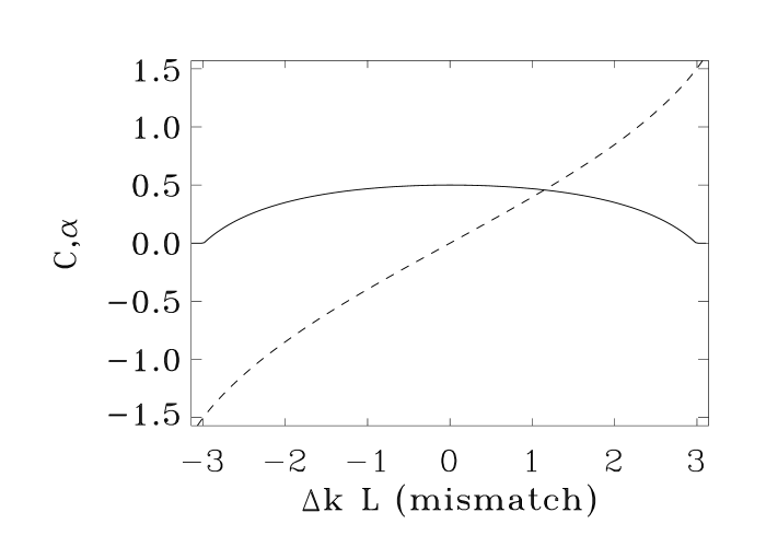
FIG. 2.:

FIG. 3.:

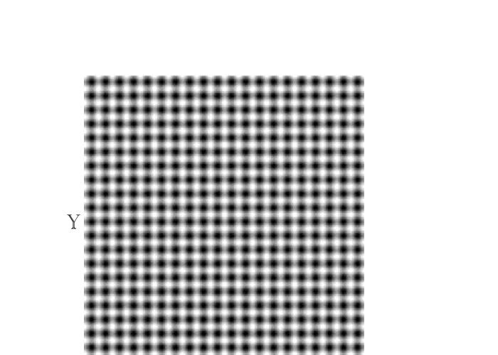
FIG. 4.:

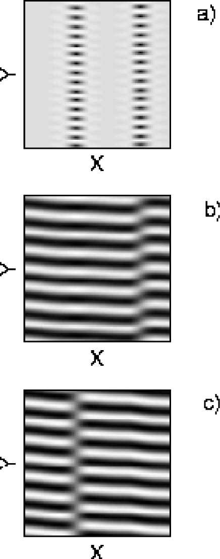
FIG. 5.:

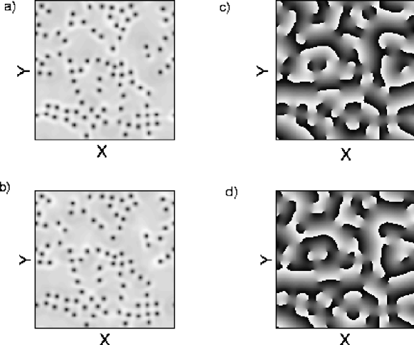
FIG. 6.:

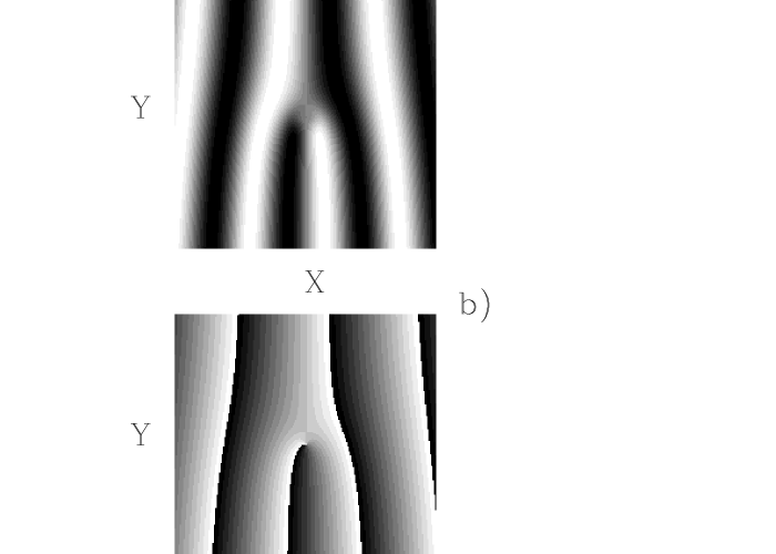
FIG. 7.:

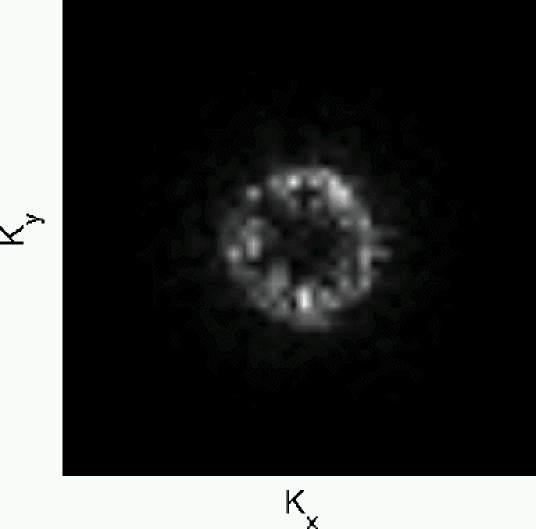
FIG. 8.:

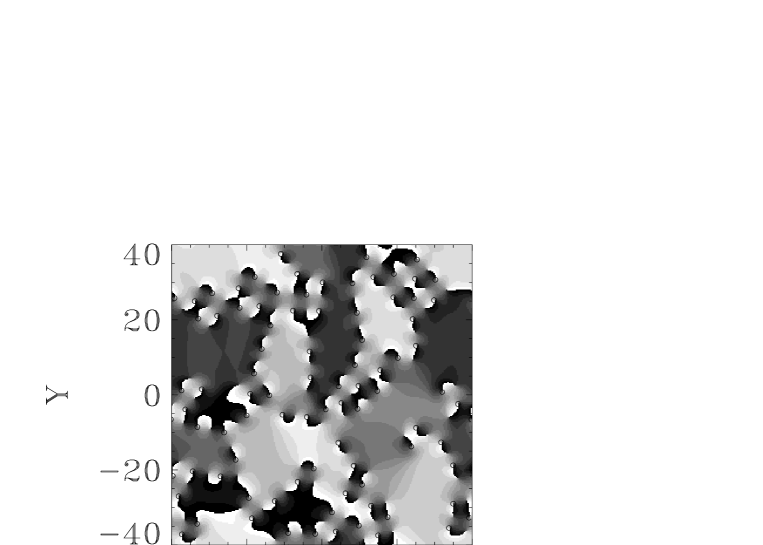
a)

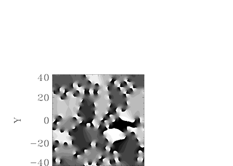
b)

FIG. 9.:

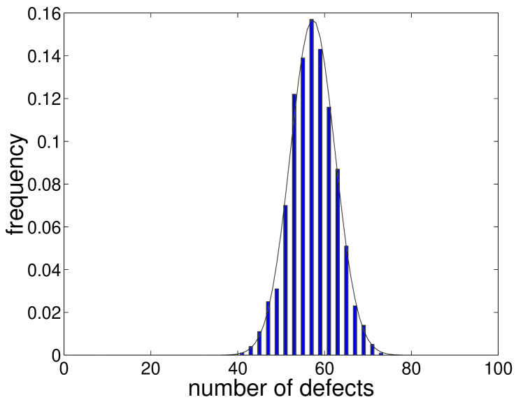
FIG. 10.:

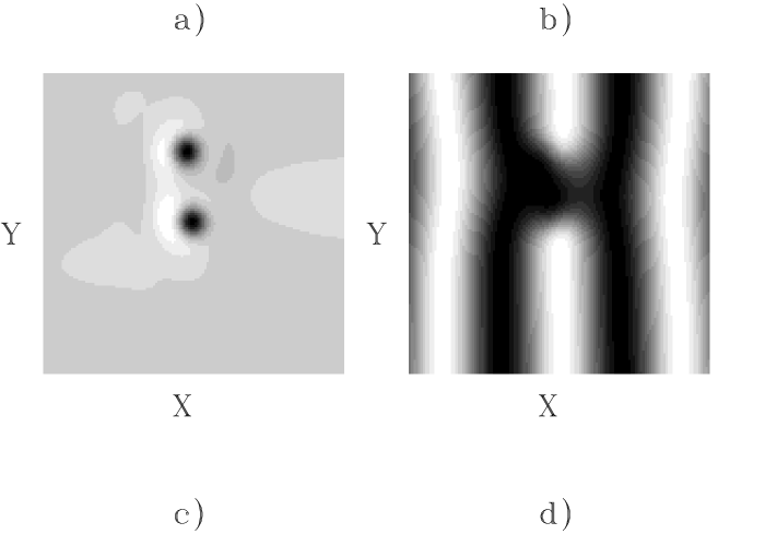
FIG. 11.:

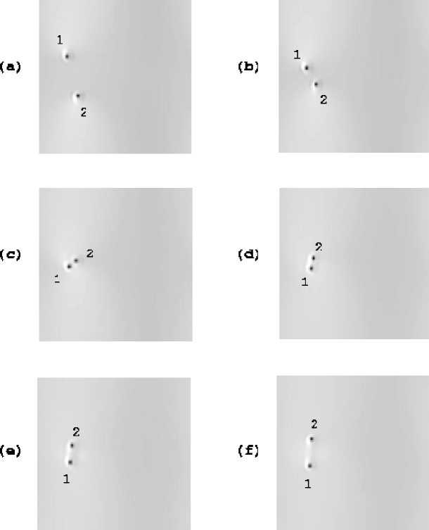
FIG. 12.:

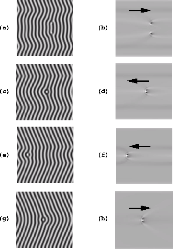
FIG. 13.:

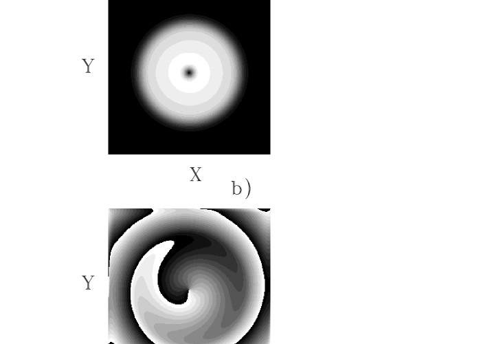
FIG. 14.:

FIG. 15.:

REFERENCES

- [1] http://www.imedea.uib.es/PhysDept
- [2] Nonlinear optical structures, patterns, chaos, ed. L.A. Lugiato special issue of Chaos, solitons and fractals 4, 1251 (1994) and references therein.
- [3] Nonlinear optical structures, patterns, chaos, ed. L.A. Lugiato special issue of Chaos, solitons and fractals 10, 617 (1999) and references therein.
- [4] Proceedings of the Euroconference: Patterns in nonlinear optical systems, Alicante (Spain) 1998 published in the special issue of Journal of Optics B: Quantum Semiclass. Opt., 1, (1999).
- [5] M. Tlidi, P. Mandel, R. Lefever, Phys. Rev. Lett. 73, 640 (1994).
- [6] M. Saffman, D. Montgomery, D. Z. Anderson, Opt. Lett. 19, 518 (1994).
- [7] W. Firth, A.J. Scroggie, Phys. Rev. Lett. 76, 1623 (1996).
- [8] N. N. Rosanov, Progress in Optics 35, 1 (1996).
- [9] A. Schreiber, B. Thuring, M. Kreuzer, T. Tschudi, Opt. Comm. 136, 415 (1997).
- [10] C. Etrich, U. Peschel, F. Lederer, Phys. Rev. Lett. 79, 2454 (1997).
- [11] K. Staliunas, J. V. Sánchez-Morcillo, Phys. Rev. A 57, 1454 (1998).
- [12] L. Spinelli, G. Tissoni, M. Brambilla, F. Prati, L. Lugiato, Phys. Rev.A 58, 2542 (1998).
- [13] C. O. Weiss, M. Vaupel, K. Staliunas, G. Slekys, V. B. Taranenko, Appl. Phys. B 68, 151 (1999).
- [14] G.-L. Oppo, A.J. Scroggie, W.J. Firth, Journal of Optics B: Quantum Semiclass. Opt. 1, 133 (1999).
- [15] M. Le Berre, D. Leduc, E. Ressayre, A. Tallet, Journal of Optics B: Quantum Semiclass. Opt., 1, 153 (1999).
- [16] B. Schapers, M. Feldmann, T. Ackemann, W. Lange, Phys. Rev. Lett., 85, 748 (2000).
- [17] P.L. Ramazza, E. Benkler, S. Boccaletti, U. Bortolozzo, S. Ducci, F.T. Arecchi, ”Tuning the properties of localized structures in a nonlinear interferometer” (Los Alamos e-print nlin.PS/0109016).
- [18] G.L. Oppo, A.J. Scroggie, W.J. Firth, Phys. Rev. E, 63, 066209 (2001).
- [19] J.B. Geddes, J.V. Moloney, E.M. Wright, W.J. Firth Opt. Comm., 111, 623 (1994).
- [20] M. Hoyuelos, P. Colet, M. San Miguel, D. Walgraef Phys. Rev. E 58, 2992 (1998).
- [21] R. Gallego, M. San Miguel, R. Toral, Phys. Rev. E 61, 2241 (2000).
- [22] A. Aumann, E. B the, Yu. A. Logvin, T. Ackemann, W. Lange, Phys. Rev. A, 56, R1709 (1997).
- [23] M. San Miguel, Phys. Rev. Lett. 75, 425 (1995).
- [24] J.Martin-Regalado, S. Balle, M. San Miguel, Optics Letters 22, 460 (1997).
- [25] E. Hernández-García, M. Hoyuelos, P. Colet, R. Montagne, M. San Miguel, Int. J. Bif. and Chaos 9, 2257 (1999); E. Hernández-García, M. Hoyuelos, P. Colet, M. San Miguel, Physical Review Letters, 85, 744 (2000).
- [26] U. Peschel, D. Michaelis, C. Etrich, F. Lederer Phys. Rev. E 58, R2745 (1998).
- [27] P. Coullet, L. Gil, F. Rocca, Opt. Comm., 73, 403 (1989).
- [28] A.B. Coates et al., Phys. Rev. A, 49, 1452 (1994).
- [29] F.T. Arecchi, G. Giacomelli, P. L. Ramazza, S. Residori, Phys. Rev. Lett., 67, 3751 (1991).
- [30] K. Staliunas, G.Slekys, C. O. Weiss, Phys. Rev. Lett., 79, 2658 (1997).
- [31] G-L. Oppo, M. Brambilla, L.A. Lugiato, Phys. Rev. A, 49, 2028 (1994).
- [32] G-L. Oppo, M. Brambilla, D. Camesasca, A. Gatti, L.A. Lugiato, J. Mod. Opt. 41, 1151 (1994).
- [33] K. Staliunas, J. Mod. Opt. 42, 1261 (1995).
- [34] S. Longhi, J. Mod. Opt. 43, 1089 (1996).
- [35] S. Longhi, J. Mod. Opt. 43, 1569 (1996).
- [36] S. Longhi, Phys. Rev. A 53, 4488 (1996).
- [37] S. Longhi, A. Geraci Phys. Rev. A 54, 4581 (1996).
- [38] G.J. de Varcarcel, K. Staliunas, E. Roldan, V.J. Sanchez-Morcillo, Phys. Rev. A 54, 1609 (1996).
- [39] V.J. Sanchez-Morcillo, E. Roldan, G.J. de Varcarcel, K. Staliunas, Phys. Rev. A 56, 3237 (1997).
- [40] M. Santagiustina, P. Colet, M. San Miguel, D. Walgraef, Phys. Rev. E 58, 3843-3853 (1998).
- [41] H. Ward, M.N. Ouarzazi, M. Taki, P. Glorieux, Eur. Phys. Journ. D. 3, 275-288 (1998).
- [42] P. Lodahl, M. Bache, M. Saffman, Phys Rev. Lett. 85, 4506 (2000).
- [43] S. Trillo, M. Haelterman, A. Sheppard, Opt. Lett., 22, 1454-1456 (1997).
- [44] S. Longhi, Phys. Scr. 57, 611 (1997).
- [45] S. Trillo, M. Haelterman, Opt. Lett. 23, 1514-1526 (1998).
- [46] M. Santagiustina, P. Colet, M. San Miguel, D. Walgraef, Opt. Lett. 23, 1167-1169 (1998).
- [47] G. Izus, M. Santagiustina, M. San Miguel, P. Colet, Jour. Opt. Soc. Am. 16, 1592 (1999).
- [48] M. Vaupel, A. Ma tre, C. Fabre, Phys. Rev. Lett., 83, 5278 (1999).
- [49] S. Ducci, N. Treps, A. Maitre, C. Fabre, Phys. Rev. A, 64, 023803 (2001).
- [50] M. Santagiustina, P. Colet, M. San Miguel, D. Walgraef, Opt. Express 3, 63-70 (1998).
- [51] M. Taki,N. Ouarzazi, H. Ward, P. Glorieux, Jour. Opt. Soc. Am. B, 17, 997 (2000).
- [52] H. Ward, M. N. Ouarzazi, M. Taki, P. Glorieux, Phys. Rev. A, 63, 016604 (2001).
- [53] G. Izus, M. Santagiustina, M. San Miguel, Opt. Lett., 25, 1454 (2000); G. Izus, M. Santagiustina, M. San Miguel ”Phase-Locked Spatial Domains and Bloch Domain Walls in Type-II Optical Parametric Oscillators”, to be published, Physical Review E (2001).
- [54] D. Michaelis, U. Peschel, F. Lederer, D. V. Skryabin, W. J. Firth, Phys. Rev. E, 63, 066602 (2001).
- [55] R.C. Eckart, C.D. Nabors, W.J. Kozlovsky, R.L. Byer, Jour. Opt. Soc. Am. B 8, 646 (1991).
- [56] J-Y Zhang, J. Huang, Y.R. Shen, ”Optical parametric generation and amplification”, in Laser Science and Technology vol 19, V.S. Letokhov, C.V. Shank, Y.R. Shen, H. Walther Eds. (Harwood Ac., 1995).
- [57] T. Debuisschert, A. Sizmann, E. Giacobino, C. Fabre, J. Opt. Soc. Am. B 10, 1668 (1993).
- [58] In our approximation the cavity is almost filled by the nonlinear crystal and thus the cavity length is very close to the crystal length.
- [59] B. E. A. Saleh, M. C. Teich, ”The fundamentals of photonics”, (Wil ey, New York 1991), Chap. 6.
- [60] Movies showing time evolution under several circumstances can be downloaded from the URL http://www.imedea.uib.es/Nonlinear/research_topics/OPO/.
- [61] M.C. Cross, P.C. Hohenberg, Reviews of Modern Physics 65, 851 (1993).
- [62] L.M. Pismen, Vortices in Nonlinear Fields, (Oxford University Press, Oxford, 1999).
- [63] A. Berzanskis, A. Matijosius, A. Piskarkas, V. Smilgevicius, A. Stabinis,Opt. Comm. 140, 273 (1997); Opt. Comm. 150, 372 (1998).
- [64] C.L. Tang, L. K. Cheng, Laser Science and Technology vol 20, V.S. Letokhov, C.V. Shank, Y.R. Shen, H. Walther Eds. (Harwood Ac., 1995).
- [65] G.I. Stegeman, M. Sheik-Bahae, E. Van Stryland, G. Assanto, Opt. Lett. 18, 13 (1993).
- [66] K.T. Gahagan, G.A. Swartzlander Jr.,Opt. Lett. 21, 827 (1996).