Statistical Properties of Fano Resonances in Atomic and Molecular Photoabsorption

Abstract

Statistical properties of Fano resonances occurring in photoabsorption to highly excited atomic or molecular states are derived. The situation with one open and one closed channel is analyzed when the classical motion of the excited complex in the closed channel is chaotic. The closed channel subspace is modeled by random matrix theory. The probability distribution of the Fano parameter is derived both for the case of time reversal symmetry (TRS) and broken time reversal symmetry. For the TRS case the area distribution under a resonance profile relevant for low resolution experiments is discussed in detail.

Introduction — Resonance phenomena are ubiquitous in highly excited quantum systems. Typical examples are auto-ionizing atomic resonances Fri98 or photodissociation of rovibrational molecular states Schi93 . When the density of resonances is high a common and natural way to extract information about resonance properties is to resort to statistical methods Haake01 ; Stoeck99 ; Guhr98 . Typically as a consequence of the high excitation the resonant complex behaves chaotically from a classical point of view. It is then appropriate to model the excited complex by means of random matrix theory BGS84 ; Alhas92 ; Alhas98 .

Here I address a problem frequently encountered in photoabsorption processes of atomic and molecular systems: What are the statistical properties of line shapes when photoabsorption into a highly excited resonant state takes place? Since the seminal work of Fano Fano61 it is known that when at least two pathways exist for an atomic or molecular system to decay after having absorbed a photon the line shapes of resonances differ in general considerably from the Breit-Wigner form. In photodissociation of molecules or photoexcitation of an atom to an auto-ionizing resonance interference between the indirect and the direct decay process results in a Beutler-Fano resonance profile of the photoabsorption cross section Fri98 ; Conn88 ; Durand01 (abbreviated as Fano profile in the following). The shape of the resonant part of the cross section is determined by a single parameter, the Fano parameter $q$. This contribution is aimed at such a statistical theory of Fano resonances.

It is worthwhile to stress that atomic and molecular systems are ideally suited to test the predictions on Fano resonances as neither Coulomb or dephasing effects which may become relevant in mesoscopic structures have to be taken into account Clerk01 .

Theory — For photodissociation of a molecule Fig. 1 schematically depicts the situation envisaged footnt1 . The molecule is coherently laser excited from the ground state or a low lying state $|0\rangle$ of energy $E_{0}$ onto two electronic potential surfaces. The transition is accomplished by the dipole operator $D$. Electronic surface S1 is the open channel — the energy $E$ of the molecular complex is above the dissociation threshold — while the motion on the potential surface S2 is bound (closed channel). The dipole matrix element for transition to the open channel is given by $d_{1}\equiv\langle 0|D|\psi_{E}^{\rm{(reg)}}\rangle$, where $|\psi_{E}^{\rm{(reg)}}\rangle$ is the regular continuum solution at energy $E$ in the open channel, normalized in energy. When $E$ coincides with the energy $E_{n}$ of a bound state $|\phi_{n}\rangle$ in the channel 2 the closed channel carries the transition amplitude $\langle 0|D|\phi_{n}\rangle$ in the absence of coupling to the continuum. In the following it is assumed that transitions between the two excited manifolds are possible. In the diabatic representation the coupling between the two surfaces is given by a non-diagonal potential $V$. Then the eigenstate $|\phi_{n}\rangle$ turns into a resonance with width $\Gamma_{n}=2\pi|\langle\psi_{E}^{\rm{(reg)}}|V|\phi_{n}\rangle|^{2}$.

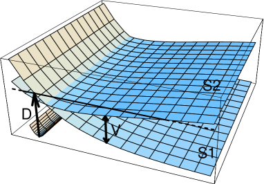
Figure 1: Schematic sketch of the photodissociation process: Laser excitation takes place from a low lying electronic potential surface (dipole operator $D$). The classical dynamics on surface S2 is bound and chaotic. Dissociation can take place directly by dipole excitation to channel 1 or indirectly by excitation to channel 2 and the coupling $V$ between the surfaces S1 and S2.

In the regime $\Gamma_{n}\ll\Delta$ of isolated resonances ($\Delta$ being the mean energy spacing of resonances) the oscillator strength $D\!f(E)$ for the dipole transition is given by Fri98

$$D\!f(E)=D\!f^{\rm(bg)}\,\frac{|q_{n}+\epsilon_{n}|^{2}}{1+\epsilon_{n}^{2}}\,,$$ (1)

where $D\!f^{\rm(bg)}\equiv 2\mu(E-E_{0})|d_{1}|^{2}/\hbar^{2}$ is the background oscillator strength for the transition to the open channel in the absence of coupling to the closed channel, $\mu$ is the reduced mass of the excited complex and $\epsilon_{n}\equiv 2(E-E_{n}-\Delta_{n})/\Gamma_{n}$ the reduced energy. The energy shift $\Delta_{n}$ of the resonance is neglected in the following. The line shape of the resonance is parameterized by the Fano parameter $q_{n}$. For a non-degenerate continuum it is given by Fri98

$$q_{n}=\frac{\langle 0|D|\phi_{n}\rangle}{\pi d_{1}\langle\psi_{E}^{\rm{(reg)}}|V|\phi_{n}\rangle}+{\overline{q}}\,,\quad{\overline{q}}=-\frac{\langle 0|D|\psi_{E}^{\rm{(irr)}}\rangle}{\langle 0|D|\psi_{E}^{\rm{(reg)}}\rangle}\,.$$ (2)

The irregular continuum solution $|\psi_{E}^{\rm{(irr)}}\rangle$ appears in the expression for $q_{n}$ because near resonance the wave function in the open channel is a superposition of the regular and the irregular solution. Both $d_{1}$ and ${\overline{q}}$ depend only weakly on $E$ and are assumed to be constant within the energy window over which a sample of resonances is taken. From (2) it is seen that the distribution of a set of Fano parameters $\{q_{n}\}$ taken over a stretch of the energy spectrum is determined by the statistical properties of the set of the eigenstates $\{|\phi_{n}\rangle\}$ of the closed channel.

The distribution of the Fano parameter is derived under the two following conditions: Firstly the classical motion of the excited molecular complex on the electronic surface S1 of the closed channel is completely chaotic. This ensures that the statistical properties of generic wave functions in chaotic systems apply and that the closed channel subspace can be modeled by random matrix theory Haake01 . Secondly the excitation process and the coupling between the two electronic surfaces are assumed to be spatially well separated: the overlap of the initial wave packet $\langle{\bf r}|D|0\rangle$ and the coupling potential $V({\bf r})$ in coordinate representation is negligible. Therefore $x\equiv\langle 0|D|\phi_{n}\rangle/d_{1}$ and $y\equiv\pi\langle\psi_{E}^{\rm{(reg)}}|V|\phi_{n}\rangle$ can be taken statistically independent random variables footnt2 .

Distribution of the Fano parameter — With these ingredients the calculation of the probability distribution $P(q)$ of the Fano parameter is straightforward. (The index $n$ of the resonance is omitted in the following.) In the case of time reversal symmetry the wave functions and viz. $x$ and $y$ can be chosen real. The closed channel subspace is modeled by $N\times N$ matrices taken from the Gaussian orthogonal ensemble (GOE). All results are understood in the limit $N\to\infty$ where $x$ and $y$ are Gaussian random random variables with zero mean and variances $\sigma_{x}^{2}$ and $\sigma_{y}^{2}$. The probability distribution is given by

$$P_{\rm GOE}(q)=\!\int\limits_{-\infty}^{\infty}\!dx\!\int\limits_{-\infty}^{\infty}\!dy\,P_{\sigma_{x}}(x)\,P_{\sigma_{y}}(y)\,\delta\!\left(q-{\overline{q}}-\frac{x}{y}\right)$$ (3)

and $P_{\sigma_{x}}(x)$ is the probability distribution of $x$ (and likewise for $y$). The integral is most easily evaluated by using the Fourier integral representation of the delta function and the result is

$$P_{\rm GOE}(q;s)=\frac{1}{\pi}\frac{s}{s^{2}+(q-{\overline{q}})^{2}}\,,\quad\quad s\equiv\sigma_{x}/\sigma_{y}\,.$$ (4)

The probability distribution of the Fano parameter in the GOE case thus turns out to be Lorentzian with mean value ${\overline{q}}$ and width $s$.

The width $s$ of the probability distribution is related to the coupling strength $V$ between the closed channel and the continuum channel and the ratio of the dipole transition matrix elements to both channels. Assume $V$ can be written in the form $V=\lambda V_{0}$ where $\lambda$ characterizes the coupling strength and $V_{0}$ is fixed. Then $\sigma_{y}\sim\lambda$ and therefore $s\sim 1/\lambda$. For strong coupling to the continuum the Lorentz distribution acquires a small width centered around ${\overline{q}}$. The same holds if direct photoexcitation dominates over the indirect process since then $\sigma_{x}$ becomes small.

In the case of broken time reversal symmetry the Hamiltonian of the closed channel is modeled by $N\times N$ matrices from the Gaussian unitary ensemble (GUE). In this case $x$ and $y$ are complex Gaussian random variables with independent real and imaginary parts and the Fano parameter is in general complex. Most conveniently the distribution of $q$ is characterized by the probability distribution of the phase $\varphi_{q}$ and the modulus $r_{q}$ of the quantity $q-\langle q\rangle$. The phases $\varphi_{x}$ of $x$ and $\varphi_{y}$ of $y$ are uniformly distributed ${\rm mod}(2\pi)$ and the same holds for $\varphi_{q}=\varphi_{x}-\varphi_{y}$. Denoting the modulus of $x$ by $r_{x}$ and of $y$ by $r_{y}$ the probability distribution $P_{\rm GUE}(r_{q})$ is given by

$$P_{\rm GUE}(r_{q})=\!\int\limits_{0}^{\infty}dr_{x}\!\int\limits_{0}^{\infty}dr_{y}\,P(r_{x})\,P(r_{y})\,\delta\!\left(r_{q}-\frac{r_{x}}{r_{y}}\right)\,,$$ (5)

where $r_{x}$ (and likewise $r_{y}$) has the probability distribution $P(r_{x})=\sigma_{r_{x}}^{-2}r_{x}\exp(-r_{x}^{2}/2\sigma_{r_{x}}^{2})$. [Notice that $P(r_{x}^{2})\sim\exp(-r_{x}^{2}/2\sigma_{r_{x}}^{2})$ has the form of a Porter-Thomas distribution for GUE.] Proceeding as in the GOE case the integrals turn out to be more complicated as they involve error functions. The final result is nevertheless simple and reads

$$P_{\rm GUE}(r_{q})=\delta(r_{q})+\frac{s_{r}^{2}r_{q}}{\left(s_{r}^{2}+r_{q}^{2}\right)^{2}}\,,\quad\quad(r_{q}\geq 0)\,,$$ (6)

where $s_{r}\equiv\sigma_{r_{x}}/\sigma_{r_{y}}$. The distribution is delta peaked at $r_{q}=0$ and has a local maximum at $r_{q}^{(0)}=s_{r}/\sqrt{3}$ with $P(r_{q}^{(0)})=3\sqrt{3}/(16s_{r})$. Again, as discussed for the GOE case the width $s_{r}$ of the probability distribution $P_{\rm GUE}(r_{q})$ is determined by the strength of the coupling between the two channels and the ratio of the strength between the dipole transition to the closed and to the open channel.

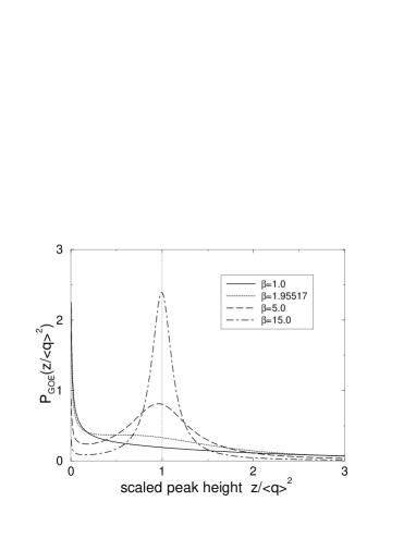
Figure 2: Peak height distribution $P_{\rm GOE}(z/{\overline{q}}^{2})$ in the GOE case for different values of $\beta={\overline{q}}/s$, $s$ being the width of the $q$-parameter distribution Eq. (4). For $\beta\geq 1.95517$ the distribution displays a local maximum between zero and one.

Peak height distribution for GOE — For the TRS case the maximum of the Fano profile is given at $\epsilon=1/q$ with peak height $z\equiv[D\!f-D\!f^{\rm(bg)}]/D\!f^{\rm(bg)}=q^{2}$ relative to the background oscillator strength. The distribution of peak heights can easily be calculated from (4) and is given by

$$P_{\rm GOE}(z)=\frac{1}{2\sqrt{z}}\left[P_{\rm GOE}(\sqrt{z};s)+P_{\rm GOE}(-\sqrt{z};s)\right]$$ (7)

with $z>0$. In Fig. 2 $P_{\rm GOE}(z)$ is plotted in terms of the scaled variable $z/{{\overline{q}}}^{2}$ and different values of the parameter $\beta={\overline{q}}/s$. It has a local maximum at a value $0<z/{\overline{q}}^{2}<1$ for $\beta\geq 1.95517$. Therefore for a local maximum to occur the width $s$ of the Lorentz profile (4) must be smaller than approximately twice the average value ${\overline{q}}$ of the Fano parameter. For $\beta\to\infty$ the position of the maximum approaches $z={\overline{q}}^{2}$.

Profile area distribution for GOE — In low resolution experiments the relevant experimental quantity is the profile area distribution under the resonance rather than the peak height distribution. To be more specific assume that the band width $\delta E$ of the exciting laser beam is larger than the width $\Gamma$ of the resonance but still smaller than the mean spacing $\Delta$ between adjacent resonances ($\Gamma<\delta E<\Delta$). Assuming a rectangular laser profile the excess oscillator strength averaged over the resonance profile with respect to the background strength is given by Bohm86

$$\overline{D\!f}^{\rm(res)}(E)=\frac{1}{\delta E}\!\!\int\limits_{E-\delta E/2}^{E+\delta E/2}\!\!D\!f^{\rm(bg)}(E^{\prime})\left[F(q;\epsilon)-1\right]dE^{\prime}$$ (8)

where $F(q;\epsilon)\equiv|q+\epsilon|^{2}/(1+\epsilon^{2})$ is the profile function of the resonance [cf. (1)]. Since $\Gamma<\delta E$ the range of integration in (8) can be extended to infinity and $\overline{D\!f}^{\rm(res)}(E)$ is given by

$$\overline{D\!f}^{\rm(res)}(E)=D\!f^{\rm(bg)}\frac{\Gamma}{2\,\delta E}\int\limits_{-\infty}^{\infty}\frac{q^{2}+2q\epsilon-1}{1+\epsilon^{2}}d\epsilon\,,$$ (9)

which performing the integration gives $\overline{D\!f}^{\rm(res)}/D\!f^{\rm(bg)}=\pi\Gamma(q^{2}-1)/2\equiv\Theta$. In the following the statistical distribution of the observable $\Theta$ is discussed. It can be written as $\Theta=x^{2}+2{\overline{q}}xy+({\overline{q}}^{2}-1)y^{2}\equiv f(x,y)$ in terms of the matrix elements $x$, $y$ and the mean value ${\overline{q}}$ of the Fano parameter. The probability distribution of $\Theta$ is given by

$$P(\Theta)=\!\!\int\limits_{-\infty}^{\infty}\!dx\,P_{\sigma_{x}}(x)\!\int\limits_{-\infty}^{\infty}\!dy\,P_{\sigma_{y}}(y)\,\delta\!\left(\Theta\!-\!f(x,y)\right)\,.$$ (10)

Introducing the scaled area ${\hat{\Theta}}\equiv a\Theta$ with $a=(\sigma_{x}\sigma_{y})^{-1}\sqrt{1/4+b^{2}}$ and $b=\left[s+s^{-1}({\overline{q}}^{2}-1)\right]/4$ the distribution $P({\hat{\Theta}})$ can be written as

$$P({\hat{\Theta}})=\frac{1}{\pi\sqrt{1+4b^{2}}}\exp(\mu{\hat{\Theta}})K_{0}(|{\hat{\Theta}}|)\,,$$ (11)

where $K_{0}$ is the MacDonald function. Additionally the asymmetry parameter $\mu=b\,[\frac{1}{4}+b^{2}]^{-1/2}$ has been introduced which determines how much $P({\hat{\Theta}})$ deviates from a symmetric distribution. $P({\hat{\Theta}})$ diverges logarithmically as ${\hat{\Theta}}$ approaches zero.

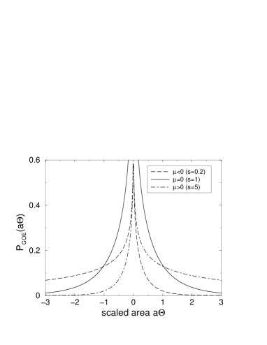
Figure 3: Distribution $P({{\hat{\Theta}}})$ of the scaled resonance area ${\hat{\Theta}}=a\Theta$, see discussion after Eq. (10). The average value of the Fano parameter is fixed at ${\overline{q}}=0$ and $s$ is varied.

Fig. 3 demonstrates the dependence of $P({\hat{\Theta}})$ at fixed ${\overline{q}}=0$ in the three characteristic regimes $\mu<0$, $\mu=0$ and $\mu>0$ by varying $s$. For $\mu=0$ the probability distribution is symmetric with respect to ${\hat{\Theta}}=0$ (solid line). For $\mu<0$ the area distribution is asymmetric with the flat side at negative values of ${\hat{\Theta}}$ (dashed line). The opposite holds for $\mu>0$ (dot-dashed line).

As $\mu$ depends both on $s$ and ${\overline{q}}$ a contour plot of $\mu$ as a function of $({\overline{q}},1/s)$ is presented in Fig. 4. The variable $1/s$ instead of $s$ has been chosen for matters of discussion as $1/s\to\infty$ corresponds to the limit of strong coupling between the closed and the continuum channel. The range of $\mu$ is $-1<\mu<1$. The white dashed line marks the subspace of parameters where $P({\hat{\Theta}})$ is symmetric $(\mu=0)$, given by ${\overline{q}}^{2}+s^{2}=1$. If $|{\overline{q}}|\geq 1$ the asymmetry parameter $\mu$ is always positive regardless of $1/s$. For fixed $|{\overline{q}}|<1$ and weak coupling ($1/s$ small) the asymmetry parameter $\mu$ is positive, too. If the coupling is enlarged $\mu$ becomes negative above a certain value of $1/s$ which depends on ${\overline{q}}$.

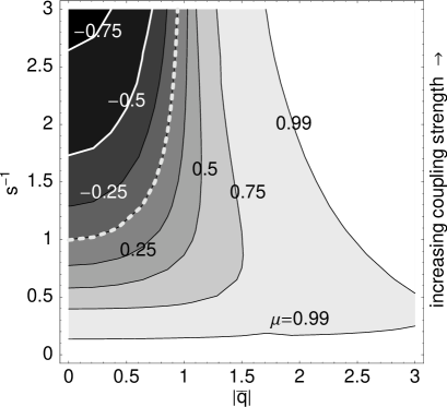
Figure 4: Asymmetry parameter $\mu$ of the area distribution, Eq. (11) as a function of the average shape parameter ${\overline{q}}$ and $s^{-1}$. The white dashed line marks the values $({\overline{q}},1/s)$ where $\mu=0$.

The expectation value of the scaled area distribution is given by $\langle{\hat{\Theta}}\rangle=\mu\,(1+4b^{2})$. Thus $\langle{\hat{\Theta}}\rangle$ is always positive when $|{\overline{q}}|\geq 1$. Note that the area under an individual resonance is positive if for its Fano parameter $|q|>1$ holds. When $|q|<1$ the area associated with an individual resonance is negative. In contrast $\langle{\hat{\Theta}}\rangle$ can either be positive or negative for $|{\overline{q}}|<1$ depending on the coupling strength to the continuum. Strong coupling to the continuum ($1/s\to\infty$) results in a negative value of $\langle{\hat{\Theta}}\rangle$. In the limit $\mu\to+1$ Breit-Wigner resonances dominate the spectrum. For fixed $|{\overline{q}}|>1$ this limit is reached both for weak and large coupling to the continuum. For $|{\overline{q}}|<1$ the Breit-Wigner limit is reached only for weak coupling ($1/s\to 0$). For $|{\overline{q}}|<1$ and strong coupling to the continuum ($1/s\to\infty$) the expectation value of the area distribution is negative and window resonances with negative area dominate the spectrum in the limit $\mu\to-1$.

Summary — Statistical properties of Fano resonances were derived for the situation of competing direct and indirect photoabsorption on the basis that the classical motion in the closed channel is chaotic. This situation is frequently encountered in photodissociation of highly excited rovibrational states of molecules or photoabsorption of atoms to auto-ionizing resonances. The closed channel subspace is modeled by random matrix theory. The distribution of the Fano parameter $q$ was derived for both the GOE and the GUE cases. The peak height distribution and the resonance area distribution were discussed in detail for the GOE.

- (1) H. Friedrich, Theoretical Atomic Physics, Springer Verlag, Berlin and Heidelberg (1998).
- (2) R. Schinke, Photodissociation Dynamics, Cambridge University Press, Cambridge (1993).
- (3) F. Haake, Quantum Signatures of Chaos, Springer Verlag, Berlin and Heidelberg (2001).
- (4) H.-J. Stöckmann, Quantum Chaos, An Introduction, Cambridge University Press, Cambridge (1999).
- (5) T. Guhr, A. Müller-Groeling and H. A. Weidenmüller, Phys. Rep. 299, 190 (1998).
- (6) O. Bohigas, M. J. Giannoni and C. Schmit, Phys. Rev. Lett. 52, 1 (1984).
- (7) Y. Alhassid and R. D. Levine, Phys. Rev. A 46, 4650 (1992),
- (8) Y. Alhassid and Y. V. Fyodorov, J. Phys. Chem. A 102, 9577 (1998).
- (9) U. Fano, Phys. Rev. 124, 1866 (1961).
- (10) J.-P. Connerade and A. M. Lane, Rep. Prog. Phys. 51, 1439 (1988).
- (11) Ph. Durand, I. Paidarová and F. X. Gadéa, J. Phys. B 34, 1953 (2001).
- (12) A. A. Clerk, X. Waintal and P. W. Brouwer, Phys. Rev. Lett. 86, 4636 (2001).
- (13) The situation is analogous for photoexcitation of an auto-ionizing atomic resonance when the system can be described by a model with one open channel and one closed chaotic channel. An example is the hydrogen atom in a homogeneous magnetic field in the chaotic regime between the first and the second Landau threshold Gremaud93 .
- (14) A. Böhm, Quantum Mechanics: Foundations and Applications, Springer Verlag, Berlin and Heidelberg (1986).
- (15) The situation where and are correlated is deferred to a future publication.
- (16) B. Grémaud, D. Delande and J. C. Gay, Phys. Rev. Lett. 70, 1615 (1993).