Reconstruction of dynamical equations for traffic flow

Abstract

Traffic flow data collected by an induction loop detector on the highway close to Köln-Nord are investigated with respect to their dynamics including the stochastic content. In particular we present a new method, with which the flow dynamics can be extracted directly from the measured data. As a result a Langevin equation for the traffic flow is obtained. From the deterministic part of the flow dynamics, stable fixed points are extracted and set into relation with common features of the fundamental diagram.

I Introduction

By increasing the number of licensed vehicles on our roads it becomes more and more necessary to reduce appearances of traffic congestion. Getting higher capacities of highways means looking for optimized flow rates of cars. In order to do so, it is necessary to investigate the complex system of traffic flow and to understand its regularities. In a subsequent step, intelligent traffic control systems may use these laws to influence the traffic flow and thus to increase the highway’s capacity utilization.

For our investigation a large amount of traffic flow data were collected at the highway near Köln-Nord (Germany) over more than one week. For each car crossing an induction loop detector the following data were recorded: (i) the time, when the car crossed the detector, with an resolution of 1 sec, (ii) the type of car (passenger car, truck), (iii) the lane number, (iv) the velocity, truncated to an 8-bit integer (0…255 km/h), accuracy of approximately 3 %, (v) the length of the car in meters (8-bit integer, not calibrated) and (vi) the distance to the car driving ahead (an integer in the range 0…999 m, not calibrated). The lanes are labeled from A to C, where lane A is the right driving lane where mostly trucks are found (because of a German law), and lanes B and C are the fast drivers’ lanes.

In the following we present a new method to derive from the measured data dynamical equations for the traffic situation. We start with the common presentation of the fundamental diagram. Next, we evaluate the deterministic and the stochastic content of of the traffic dynamics by means of a Langevin equation. Finally, we give an interpretation of the determined Langevin equation.

II Fundamental diagrams

Here and in the following we calculate the car density $k$ [km^-1] and the flux state $q$ [h^-1] of each car using the measured data: the velocity $v$ [km/h], the length of the car $l$ [m] and the distance $d$ [m] to the car ahead:

$$k = \frac{1000}{l+d}\;\;,$$ (1)

$$q = k\cdot v\;\;.$$ (2)

To avoid an overload of the presentation we restrict the diagrams and the following calculations to two cases. Firstly, only the traffic of a single lane C, secondly the cumulative traffic of all three lanes A, B and C are considered. Furthermore we calculate for each density state $k$ the mean flux state

$$\langle q\rangle_{k}=\frac{1}{n(k)}\sum q(k)\;\;.$$ (3)

The obtained fundamental diagrams (q_i;k_i) and ($<$q$>$;k) are shown in Fig. 1. We note that for this presentation no significant difference in the traffic dynamics of one lane and the cumulative dynamics of three lanes can be detected. In both diagrams we find a maximum flux in free traffic flow of $q_{\rm max}=8000$ cars/h, according to the results of [1]. For the flux out of traffic jams we find in both cases $q_{\rm out}=5000$ cars/h. So we have a ratio of $\eta:=q^{\rm free}_{\rm max}/q_{\rm out}=1.6$, which meets the value $\eta\approx 1.5$ found in [1] quite well.

III Langevin equation for the traffic flow

In order to grasp the underlying dynamics of the traffic flow (one lane and all three lanes), we utilize a new method to analyze the traffic data more extensively. In particular, the iterative dynamics of the traffic state ${\mathbf{x}}_{N}$, given by the velocity ${\mathbf{v}}_{N}$ and the flux ${\mathbf{q}}_{N}$ of the $N$-th car, as a function of traffic state ${\mathbf{x}}_{N-1}$ of the $N-1$-th car is investigated. Note, that other state variables could have been choosen as well.

For the iterative dynamics of the traffic state ${\bf x}_{N}$ (which may be taken in a generalized case as a $r$-dimensional variable) we propose a description by a stationary Langevin equation, taking into account a combination of deterministic and random (noisy) forces cf. [2]:

$$x_{i,N+1}=x_{i,N}+h_{i}({\bf x}_{N})+\sum_{j=1}^{r}g_{ij}({\bf x}_{N})\cdot\Gamma_{j,N}\;\;,$$ (4)

where the indices $i$ and $j$ denote components of the multidimensional variables, $N$ the time, and $\Gamma_{j,N}$ are $r\times N$ independent Gaussian noise variables with zero mean and with variance 2, i.e.,

$$\langle\Gamma_{j,N}\rangle=0\;,\;\;\langle\Gamma_{j,M}\cdot\Gamma_{k,N}\rangle=2\delta_{j,k}\delta_{M,N}\;\;.$$ (5)

The central part of our following work is that it is possible to determine the functions $h_{i}$ and $g_{ij}$ directly from empirical data. Taking (4) as the Ito presentation of the stochastic process the following relation to the Kramers-Moyal coefficients can be given,

$$D_{i}^{(1)}({\bf x}) = h_{i}({\bf x})$$ (6)

$$D_{ij}^{(2)}({\bf x}) = \sum_{k=1}^{r}g_{ik}({\bf x})g_{jk}({\bf x})\;\;,$$ (7)

where $D^{(1)}$ and $D^{(2)}$ are called drift and diffusion coefficient. These coefficients can be evaluated by the conditional moments

$$D_{i}^{(1)}({\bf x})=\langle x_{i,N+1}-x_{i}\rangle\Big{|}_{{\bf x}_{N}={\bf x}}\;\;,$$ (8)

$$D_{ij}^{(2)}({\bf x})=\langle(x_{i,N+1}-x_{i})(x_{j,N+1}-x_{j})\rangle\Big{|}_{{\bf x}_{N}={\bf x}}\;\;.$$ (9)

Recently it has been shown that with the analogous definition of these Kramers-Moyal coefficients it is possible to reconstruct from time continuous dynamics the underling stochastic differential equation [3].

Before presenting our results on the dynamics we want to comment on the validity of this ansatz to describe the traffic flow by the Langevin equation (4). This ansatz implies that the dynamics is in the class of Markovian processes, i.e. the system does not have a memory. This can be tested by conditional probabilities

$$p(\bf{x}_{N}|\bf{x}_{N-1},\ldots,\bf{x}_{N-m})=p(\bf{x}_{N}|\bf{x}_{N-1})$$ (10)

or by the necessary condition of the Chapman-Kolmogorov equation

$$p(\bf{x}_{N}|\bf{x}_{N-r})=\sum_{\bf{x}_{N-s}}p(\bf{x}_{N}|\bf{x}_{N-s})p(\bf{x}_{N-s}|\bf{x}_{N-r})\;\;,$$ (11)

where $r>s$. From our data, conditional probabilities have been evaluated and the validity of the Chapman-Kolmogorov equation was found for the iterative dynamics of both quantities, the velocity and the flux. If this Markovian property holds, the inherent noise of the dynamics ($\Gamma$) can be taken as $\delta$-correlated. It should be noted, that even in the case where the noise is not $\delta$-correlated, the deterministic part of the dynamics can be reconstructed from given data (8), as we found by analysing numerically generated test data, [4].

As expressed by (9), the knowledge of the conditional probabilities $p(\bf{x}_{N}|\bf{x}_{N-1})$ provides the basis to estimate the Kramers-Moyal coefficients from the traffic data. First we consider the simplified case of the onedimensional dynamics of the velocity only. The results for and $D^{(2)}$(v) for the traffic of one lane and for the cumulative traffic of all three lanes are shown in Fig. 2. The one dimensional deterministic dynamics can also be expressed by the potential $\Phi_{D}$(v), defined as - $\frac{\delta\Phi_{D}}{\delta v}$ = D⁽¹⁾(v). The corresponding potentials are shown in Fig. 3. From these results three noticable velocities $v_{1}\approx 37$ km/h, $v_{2}\approx$ 75 km/h and $v_{3}\approx$ 107 km/h appear, which allows to identify the so called congested flow for $v\leq v_{1}$, correlated flow for $v_{1}<v\leq v_{2}$ and the free flow for $v>v_{2}$ [5, 7], respectively. Note these velocities can be defined as fixed points ($D^{(1)}(v)=0$) of the deterministic part of the cumulative traffic dynamics (see Fig. 2b).

For the traffic dynamics of lane C we find in the congested and in the correlated regime metastable traffic states, the deterministic drift term $D^{(1)}$ gets zero over finite intervals. This corresponds to the plateau structure in the potential, see Fig. 3a. A clearly different behaviour is found for the cumulative traffic dynamics of all three lanes, see Figs. 2b and 3b. The different flow regimes are seperated by two fixed points at $v_{1}$ and $v_{2}$. The slope of these fixed points defines the stability, thus the congested and the correlated flow regimes are separated by a stable fixed point, whereas the correlated and the free flow regime are separated by an instable fixed point. For the free flow, in both cases of one lane or three lane traffic a stable fixed point is found at $v_{3}$, correspondingly the drift potential has its local minimum. Because of a speed limit of 100 km/h given on the inspected highway we see a great increase of the potential for $v>v_{3}$: the faster a car is driving, the stronger the attraction is to the potential’s minimum [6] .

To get an understanding of the real traffic dynamics grasped by these drift coefficients or drift potentials, the additional noise has to be taken into account. In Fig. 2c and d the corresponding magnitude of the noise are expressed by the evalutaed diffusion coefficients $D^{(2)}$. The noise will now cause transitions between different flow states. For the traffics dynamics of one lane, the noise will effect larger fluctuations as it is the case for the cumulative traffic dynamics, which has two clear minima in the potential. A further interesting detail is that the magnitude of $D^{(2)}$ has a minimum around the stable fixed point at $v_{3}$. This indicates a pronounced stability of this traffic situation.

Next we present the results of a higher dimensional analysis by taking ${\bf x}$ with the components $x_{1}=v$ and $x_{2}=q$. Now also the drift coefficient $D^{(1)}$ becomes a vector depending on $v$ and $q$, as shown in Fig. 4. These results were obtained by binning the velocity flux data into a $25\times 25$ matrix, corresponding to a binning of the velocity into intervals of $\Delta\,v=5$ km/h.

The solid lines in Fig. 4 show the states where we have no drift of the flux component: $D_{q}^{(1)}=0$. On these lines we find only a velocity drift with a constant flux. In accordance to Fig. 2a we find in Fig. 4a for slow velocities mainly no velocity drift, in Fig. 4b (like in Fig. 2b) there seem to exist stable velocity drift states at the same velocities ($v_{i}\approx 37$km/h,$107$ km/h). The topology of the instable fixed point gets now a saddle point which is attractive for larger and smaller flux values but instable in the direction of larger and smaller velocity values. Again clear differences of the dynamics of on lane and three lanes is found.

IV Discussion and Conclusion

By the investigation of traffic flow data as an iterative stochastic process we were able to calculate from the given data the 1-dimensional drift and diffusion coefficients and thus to find the deterministic and stochastic part of the corresponding Langevin equation. We are able to find stable, metastable and unstable states (fixed points) in the deterministic part of free, correlated and congested traffic flow. For a fully description of the whole dynamics also the diffusion coefficient has to be taken into account, which provides transition probabilities between the different (meta-)stable states. Without this noisy part of the traffic flow dynamics, the stable states would never be left, i.e. a congestion would stay forever if once prepared.

To see the dependency of velocity and flow from each other, the investigations were expanded to a higher dimensional analysis. In this case we find the deterministic and stochastic part of the 2-dimensional Langevin equation. Now we are able to identify stable velocity and flux states of the deterministic part.

Interestingly, the results found in this study are in agreement with empirical investigations that have identified three phases of traffic [8], together with transitions connecting theses phases. Especially the transition from free flow to correlated flow (or synchronized flow in the terminology of [8]) has similarities.

Finally we want to point out, that we presented here a new method to analyse traffic data with respect to a derivation of dynamical equations from pure data analysis. Furthermore we could show that our method provides more insight into the traffic dynamics than the presentations of diagrams like the fundamental diagram. A clear difference in the dynamics of one lane and the dynamics of cumulative three lanes was found. Our analysis provides evidence of the presence of fixed points, which are of practical importance if a control of a traffic should be achieved. At last one may conclude that this method will be helpful to perform a more thorough comparison between traffic flow models and empirical data.

Acknowledgement: Helpful discussions with Ch. Renner, St. Lück and M. Siefert are acknowledged. We also would like to thank the Landschaftsverband Rheinland and the Northrhine-Westfalia Ministry for Economy and Transport for providing the data used in this study.

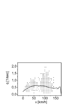
FIG. 1.: Fundamental diagram of (a) lane C and of (b) all three lanes A,B, and C. The dots represent the measured traffic data, the solid line corresponds to the mean flux $\langle q\rangle_{k}$.

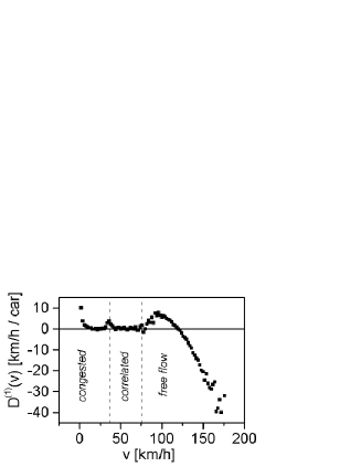
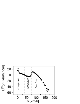
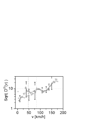
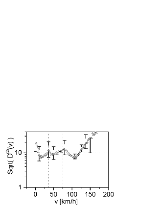
FIG. 2.: Drift and diffusion coefficients for the traffic of one lane C, (a) and (c) and of all three lanes (b) and (d).

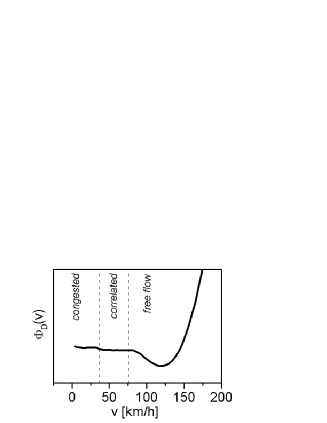
FIG. 3.: Corresponding potentials for the deterministic dynamics given by the drift coefficients in Fig. 2.

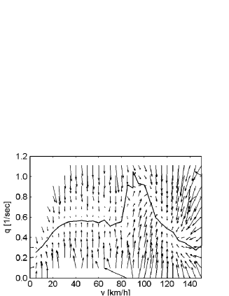
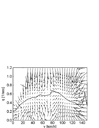
FIG. 4.: Deterministic dynamics of the twodimensional traffic states $(q,v)$ given by the drift vector for (a) one lane C and (b) all three lanes. Bold dots indicate stable fixed points and open dots saddle points, respectively.

REFERENCES

- [1] B. S. Kerner, Traffic Flow, Experiment and Theory, in Proceedings of the Workshop on Traffic and Granular Flow ’97, (Springer Verlag, Berlin, 1998) pp. 239-267
- [2] H. Risken, The Fokker–Planck Equation (Springer, Berlin, 1989).
- [3] S. Siegert, R. Friedrich, and J. Peinke, Phys. Lett. A 243, 275 (1998); 271, 217 (2000).
- [4] M. Siefert, Diplomarbeit Oldenburg, 2000.
- [5] B. S. Kerner, Phys. Rev. Lett. 81, 3797 (1998).
- [6] It is commonly known, that in Germany people like to drive about 10 percent faster than given speed limits. With this speed there is still no punishment by the police.
- [7] L. Neubert, L. Santen, A. Schadschneider, and M. Schreckenberg, Phys. Rev. E 60 6480 (1999).
- [8] B. S. Kerner, J. Phys. A 33, L221-L228 (2000).