Zipf’s law in human heartbeat dynamics

Abstract

It is shown that the distribution of low variability periods in the activity of human heart rate typically follows a multi-scaling Zipf’s law. The presence or failure of a power law, as well as the values of the scaling exponents, are personal characteristics depending on the daily habits of the subjects. Meanwhile, the distribution function of the low-variability periods as a whole discriminates efficiently between various heart pathologies. This new technique is also applicable to other non-linear time-series and reflects these aspects of the underlying intermittent dynamics, which are not covered by other methods of linear- and nonlinear analysis.

The nonlinear and scale-invariant aspects of the heart rate variability (HRV) have been studied intensively during the last decades. This continuous interest to the HRV can be attributed to the controversial state of affairs: on the one hand, the nonlinear and scale-invariant analysis of HRV has resulted in many methods of very high prognostic performance (at least on test groups) Amaral ; Ivanov ; Thurner ; Saermark ; on the other hand, practical medicine is still confident to the traditional “linear” methods. The situation is quite different from what has been observed three decades ago, when the “linear” measures of HRV became widely used as important noninvasive diagnostic and prognostic tools, soon after the pioneering paper Hon . Apparently, there is a need for further evidences for the superiority of new methods and for the resolution of the existing ambiguities.

During recent years the main attention of studies has been focused on the analysis of the scale-invariant methods. It has been argued that measures related to a certain time-scale (e.g. 5 min) are less reliable, because the characteristic time-scales of physiological processes are patient-specific. The scale-invariant measures are often believed to be more universal and sensitive to life-threatening pathologies Amaral ; Ivanov . However, carefully designed time-scale-related measures can be also highly successful, because certain physiological processes are related to a specific time scale Thurner .

The scale invariance has been exclusively seen in the heart rhythm following the (multi)fractional Brownian motion (fBm) Peng . It has been understood that the heart rhythm fluctuates in a very complex manner and reflects the activities of the subject (sleeping, watching TV, walking etc.) Poon ; Struzik and cannot be adequately described by a single Hurst exponent of a simple fBm. In order to reflect the complex behavior of the heart rhythm, the multi-affine generalization of the fBm has been invoked Amaral ; Ivanov ; it has been claimed that the multifractal scaling exponents are of a significant prognostic value.

The approach based on fBm addresses long-time dynamics of the heart rhythm while completely neglecting the short-scale dynamics on time scales less than one minute (the respective frequencies are typically filtered out Peng ). The short-time variability has been described only by the so called linear measures, such as $p_{NN50}$ (the probability that two adjacent normal heart beat intervals differ more than 50 milliseconds). Meanwhile, the level of the short-time variability of the human heart rate varies in a very complex manner, the high- and low-variability periods are deeply intertwined Poon . This is a very important aspect, because the low-variability periods are the periods when the heart is in a stressed state, with high level of signals arriving from the autonomous nervous system. The conventional linear measures are not appropriate for describing such a complex behavior. Thus, there is a clear need for suitable nonlinear methods.

In this paper we present a new scale-invariant description of the short-time variability of the heart rate. It is shown that the distribution of low-variability periods in the activity of a normal heart follows the Zipf’s law. It is also shown that the distribution function of the low-variability periods contains a considerable amount of diagnostically valuable information. This new technique is also applicable to other non-linear time-series, such as EEG signals and financial data KSK .

Our analysis is based on ambulatory Holter-monitoring data (recorded at Tallinn Diagnostic Centre) of 218 patients with various diagnoses. The groups of patients are shown in Table 1. The sampling rate of ECG was 180 Hz. The patients were monitored during 24 hour under normal daily activities. The preliminary analysis of the ECG recordings was performed using the commercial software; this resulted in the sequence of the normal-to-normal (NN) intervals $t_{NN}$ (measured in milliseconds), which are defined as the intervals between two subsequent normal heartbeats (i.e. normal QRS complexes).

	Healthy	IHD	SND	VES	PCI	RR	FSK
No. of patients	103	8	11	16	7	11	6
Mean age	$45.5$	$65.4$	$50.0$	$55.9$	$47.3$	$55.5$	$11.7$
Std. dev. of age	$20.5$	$11.4$	$19.3$	$14.3$	$11.6$	$14.4$	$4.6$

Table 1: Test groups of patients. Abbreviations are as follows: IHD - Ischemic Heart Disease (Stenocardia); SND - Sinus Node Disease; VES - Ventricular Extrasystole; PCI - Post Cardiac Infarction; RR - Blood Pressure Disease; FSK - Functional Disease of Sinus Node.

Originally, the Zipf’s law addressed the distribution of words in a language Zipf : every word has assigned a rank, according to its “size” $f$, defined as the relative number of occurrences in some long text (the most frequent word obtains rank $r=1$, the second frequent — $r=2$, etc). The empirical size-rank distribution law $f(r)\propto r^{-\alpha}$ is surprisingly universal: in addition to all the tested natural languages, it applies also to many other phenomena. The scaling exponent $\alpha$ is often close to one (e.g. for the distribution of words). Typically, the Zipf’s law is applicable to a dynamical system at statistical equilibrium, when the following conditions are satisfied: (a) the system consists of elements of different size; (b) the element size has upper and lower bounds; (c) there is no intermediate intrinsic size for the elements. As already mentioned, the human heart rhythm has a complex structure, where the duration $\tau$ of the low-variability periods varies in a wide range of scales, from few to several hundreds of heart beats. Thus, one can expect that the distribution of the low-variability periods follows the Zipf’s law

$$r\propto\tau^{-\gamma}.$$ (1)

However, the scaling behavior should not be expected to be perfect. Indeed, the heart rate is a non-stationary signal affected by the non-reproducible daily activities of the subjects. The non-stationary pattern of these activities, together with their time-scales, is directly reflected in the above mentioned distribution law. This distribution law can also have a fingerprint of the characteristic time-scale (around ten to twenty seconds) of the blood pressure oscillations. Finally, there is a generic reason why the Zipf’s law fails (or is non-perfect) at small rank numbers. The Zipf’s law is a statistical law; meanwhile, each rank-length curve is based on a single measurement. Particularly, there is only one longest low-variability period (and likewise, only one most-frequent word), the length of which is just as long as it happens to be, there is no averaging whatsoever. For large rank values $r$, the relative statistical uncertainty can be estimated as $1/\sqrt{r}$.

To begin with, we define the local variability for each ($i$-th) interbeat interval as the deviation of the heart rate from the local average,

$$\delta(i)=\frac{|t_{NN}(i)-\left<t_{NN}(i)\right>|}{\left<t_{NN}(i)\right>}.$$ (2)

The angular braces denote the local average, calculated using a narrow (5 beats wide) Gaussian weight function. Further, we introduce a threshold value $\delta_{0}$; $i$-th interbeat interval is said to have a low variability, if the condition

$$\delta(i)\leq\delta_{0}$$ (3)

is satisfied. A low-variability period is defined as a set of consecutive low-variability intervals; its length $\tau$ is measured in the number of heartbeats. Finally, all the low-variability periods are arranged according to their lengths and associated with ranks. The rank of a period is plotted versus its length in a logarithmic graph, see Fig. 1; Zipf’s law would correspond to a straight descending line.

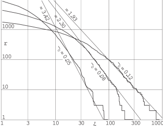
Figure 1: Multi-scaling distribution of the low-variability periods: the rank $r$ of a period is plotted versus its duration $\tau$ (measured in heartbeats) for different values of the threshold parameter $\delta_{0}$.

For a very low threshold parameter $\delta_{0}$, all the low-variability periods are very short, because it is difficult to satisfy the stringent condition (3). In that case, the inertial range of scales is too short for a meaningful scaling law. On the other hand, for a very high value of $\delta_{0}$, there is a single low-variability period occupying the entire HRV-recording. Between these two cases, there is such a range of the values of $\delta_{0}$, which leads to a non-trivial rank-length law. For a typical healthy patient, the $r(\tau)$-curve is reasonably close to a straight line, and the scaling exponent $\gamma$ is a function of the threshold parameter $\delta_{0}$. Thus, unlike all the other well-known applications of the Zipf’s law, we are dealing with a multi-scaling law.

Recently, Ivanov et. al. Ivanov have reported that anomalous multifractal spectra of the HRV signal indicate an increased risk of sudden cardiac death. Therefore, it is natural to ask, does the presence or failure of the multiscaling behavior indicate the healthiness of the patient? In what follows we discuss a somewhat more general question: what is the relationship between the properties of the distribution function of the low variability periods and the diagnosis of the patient. Testing the prognostic significance for predicting sudden cardiac death, which is also of a great importance, has been postponed due to the nature of our test groups.

First, let us analyze the correlation between the diagnosis of a patient and the scaling exponent $\gamma$. To begin with, we have to determine the optimal value for the threshold parameter $\delta_{0}$. For a meaningful analysis, the scaling behavior should be as good as possible. It turned out that for a typical patient, the best approximation of the function $r(\tau)$ with a power law is achieved for $\delta_{0}\approx 0.05$ (see Fig. 2a); in what follows, all the values of the exponent $\gamma$ are calculated for $\delta_{0}=0.05$. It should be noted that for some patients, the length-rank distribution is still far from a power law (see Fig. 2b).

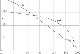
Figure 2: Rank-length curves for a patient with a good power law (a) and for a patient with no power law (b). In both cases, the threshold parameter $\delta_{0}=0.05$.

The slope of a curve on the logarithmic plot is calculated using root-mean-square (rms) fit for such a range of lengths $[\tau_{\mbox{\scriptsize start}},\tau_{\mbox{\scriptsize end}}]$, for which the $r(\tau)$-curve is nearly a power law, and the scaling range width $\Delta=\ln\tau_{\mbox{\scriptsize end}}-\ln\tau_{\mbox{\scriptsize start}}$ is as large as possible. Bearing in mind the statistical nature of the Zipf’s law and non-stationarity of the underlying signal, we have chosen a not very stringent definition of what is “nearly a power law”, see Fig. 3. Around the rms-fit-line, two limit lines are drawn; $\tau_{\mbox{\scriptsize start}}$ and $\tau_{\mbox{\scriptsize end}}$ correspond to the points, where the $r(\tau)$-curve crosses the limit lines.

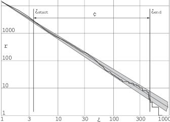
Figure 3: Definition of the width of the scaling interval $\Delta$. The rank-length curve is fitted with a power law; the boundaries of the scaling interval are defined as the intersection points of limit lines and $r(\tau)$-curve.

Note that the precise placement and shape of the limit lines is arbitrary, i.e. small variations do not lead to qualitative effects. Here, the distance of the limit lines from the central line has been chosen to be $\ln 2$ at $\tau=\tau_{\max}$, and zero at $\tau=1$, where $\tau_{\max}$ is the length of the longest low-variability period. Admitting mismatch $\ln 2$ at $\tau=\tau_{\max}$ is motivated by the observation that due to the lack of any statistics, the longest low-variability period could have been easily twice as long as we measured it to be. For large rank values, the statistical uncertainty is assessed as $\sqrt{r}$; in logarithmic graph, this would correspond to an exponentially decreasing (with increasing $r$) distance between a limit curve and the central fit-line. However, the above mentioned effect of the non-stationary pattern of the subjects daily activities makes the situation more complicated. There is no easy way to quantify this effect and therefore, we opted for the simplest possible solution, simple straight limit lines.

The scaling exponent $\gamma$ has been calculated for all the patients and Student test was applied to every pair of groups. In most cases, the significance was quite low; two best distinguishable groups were RR and FSK, the result of Student test being 5.7%. Therefore, one can argue that the slopes of linear parts are highly personal characteristics depending also on the daily habits of the subjects, which are weakly correlated with diagnosis.

Further we tested, how is the failure of the power law correlated with the diagnosis. The width of the scaling range $\Delta$ was used as a measure of how well the curve is corresponding to a power law. The Student test results for the parameter $\Delta$ turned out to be similar to what has been observed for the parameter $\gamma$: the correlation between the failure of the power law and diagnosis was weak. Thus, a rank-length curve resembling the one depicted by a dashed line in Fig. 2, does not hint to heart pathology. It should be also noted that the dashed curve in Fig. 2 can be considered as a generalized form of scale-invariance with scale-dependent differential scaling exponent. Such a behavior seems to be universal; for instance, certain forest fire models Chen lead to the differential fractal dimension depending on the local scale.

Finally, we analyzed the diagnostic significance of the parameters $\ln\tau_{\mbox{\scriptsize end}}$ and $\ln\tau_{\mbox{\scriptsize start}}$. This analysis does make sense, because typically, the start- and end-points of the scaling range correspond to certain physiological time-scales. The parameter $\ln\tau_{\mbox{\scriptsize end}}$ provided, indeed, a remarkable resolution between the groups of patients, see Table 2. According to the Student test, the healthy patients, were distinct from five heart pathology groups with probability $p<1.6$%. The parameter $\ln\tau_{\mbox{\scriptsize start}}$ was diagnostically less significant.

Table 2: $p$-values of the Student test. Data in the topmost triangular region (with label A) are calculated using the parameter $\ln\tau_{\mbox{\scriptsize end}}$. Triangular region B corresponds to the parameter $\ln r_{\max}$, region C — to $\ln r_{100}$, and region D — to $\ln\tau_{40}$. Gray background highlights small $p$-values, $p<10\%$.

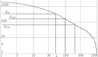
Figure 4: Definition of the parameters $r_{50}$, $r_{100}$, and $r_{200}$.

Unfortunately, the calculation of the parameter $\tau_{\mbox{\scriptsize end}}$ is technically quite a complicated task, not suited for clinical practice. Therefore, we aimed to find a simpler alternative to it. Basically, the strategy was to find a simple parameter reflecting the behavior of the rightmost (large-$\tau$) part of the $r(\tau)$-curve. An easy option is $\ln\tau_{\max}$, which has been already analyzed JKMS . This parameter has indeed a considerable diagnostic value, but its reliability is decreased by the above discussed statistical fluctuations. Better alternatives are provided by (a) the overall number of low-variability periods $r_{\max}$ (which is small, if there are lot of long low-variability periods); (b) the coordinates of specific points of the rank-length curve. Here we chose a set of critical ranks $R=10$, $20$ or $40$, and determined the respective lengths $\tau_{R}$ so that $r(\tau_{R})=R$. We also fixed a set of critical length values, $T=50$, $100$, or $200$, and determined the respective rank numbers $r_{T}=r(T)$, see Fig. 4. Both techniques turned out to be of high diagnostic performance; illustrative $p$-values are given in Table 2. Parameters $\tau_{10}$ and $\tau_{20}$ performed less well than $\tau_{40}$ (for instance, the $p$-values for the healthy and VES-subject groups were 0.60%, 0.58% and 0.34%, respectively), and are not presented in tabular data. Similarly, $r_{100}$ turned out to be more efficient than $r_{50}$ and $r_{200}$ (the respective healthy and VES-group $p$-values being $0.02$%, $0.01$%, and $0.09$%). It also outperforms $\tau_{40}$, but is sometimes less efficient than $r_{\max}$ or $\tau_{\mbox{\scriptsize end}}$ (see Table 2). Hence, various heart pathologies seem to affect the heart rate dynamics at the time scale around 100 heart beats (one to two minutes).

In conclusion, new aspect of non-linear time-series has been discovered, the scale-invariance of low-variability periods. We have shown that the distribution of low variability periods in the activity of human heart rate typically follows a multi-scaling Zipf’s law. The presence or failure of a power law, as well as the values of the scaling exponents, are personal characteristics depending on the daily habits of the subjects. Meanwhile, the distribution function of the low-variability periods as a whole contains also a significant amount of diagnostically valuable information, the most part of which is reflected by the parameters $r_{100}$, $r_{\max}$, and $\tau_{\mbox{\scriptsize end}}$, see Table 2. These quantities characterize the complex structure of HRV signal, where the low- and high variability periods are deeply intertwined, aspect which is not covered by the other methods of heart rate variability analysis (such as fractional Brownian motion based multifractal analysis). As a future development, it would be of great importance to analyze the prognostic value of the above mentioned parameters for patients with sudden cardiac death.

The support of ESF grant No. 4151 is acknowledged.

References

- (1) L.A.N. Amaral, A.L. Goldberger, P.Ch. Ivanov, and H.E. Stanley, Phys. Rev. Lett. 81, 2388,(1998).
- (2) P.Ch. Ivanov et al, Nature, 399, 461 (1999).
- (3) S. Thurner, M.C. Feurstein, and M.C. Teich, Phys. Rev. Lett. 70, 1544,(1998).
- (4) K. Saermark et al, Fractals, 8, 315,(2000).
- (5) E.H. Hon and S.T. Lee, Am. J. Obstet. Gynec. 87, 814, (1965).
- (6) C.K. Peng et al., Phys. Rev. Lett. 70, 1343,(1993).
- (7) C.S. Poon and C.K. Merrill, Nature, 389, 492,(1997).
- (8) J. Kalda, M. Säkki, R. Kitt, unpublished.
- (9) Z.R. Struzik, Fractals, 9, 77(2001).
- (10) K. Chen and P. Bak, Phys. Rev. E, 62, 1613 (2000).
- (11) J. Kalda, M. Vainu, and M. Säkki, Med. Biol. Eng. Comp. 37, 69(1999).
- (12) G.K. Zipf, Human Behavior and the Principle of Least Effort (Cambridge, Addison-Wesley, 1949).