Internal energy of high density Hydrogen: Analytical approximations compared with path integral Monte Carlo calculations

Abstract

The internal energy of high-density hydrogen plasmas in the temperature range $T=10,000\dots 50,000K$ is calculated by two different analytical approximation schemes (method of effective ion-ion interaction potential - EIIP and Padé approach within the chemical picture - PACH) and compared with path integral Monte Carlo results. Reasonable agreement between the results obtained from the three independent calculations is found, the reasons for still existing differences is investigated. Interesting high density phenomena such as the formation of clusters and the onset of crystallization are discussed.

I Introduction

The thermodynamics of strongly correlated Fermi systems at high pressure are of growing importance in many fields, including shock and laser plasmas, astrophysics, solids and nuclear matter, see Refs. [1, 2, 3, 4, 5] for an overview. In particular, the thermodynamic properties of hot dense plasmas are essential for the description of plasmas generated by strong lasers [5]. Further, among the phenomena of current interest are the high-pressure compressibility of deuterium [6], metallization of hydrogen [7], plasma phase transition etc., which occur in situations where both interaction and quantum effects are relevant. Among the early theoretical papers on dense hydrogen we refer to Wigner/Huntington [8], Abrikosov [9], Ashcroft [10] and Brovman et al. [11] and, concerning the plasma phase transition, see Norman and Starostin [12], Kremp et al. [13], Saumon and Chabrier [14] and Schlanges et al. [15], as well as to some earlier investigations of one of us [16, 17, 18, 19]. Among the early simulation approaches we refer to several Monte Carlo (MC) calculations, e.g. [20, 21, 22].

There has been significant progress in recent years in studying these systems analytically and numerically, see e.g. [1, 2, 4, 23, 24, 25, 26, 27] for an overview. However, there remains an urgent need to test analytical models by an independent numerical approach. Besides the molecular dynamics approach, e.g. [23, 25], the path integral Monte Carlo (PIMC) method is particularly well suited to describe thermodynamic properties in the region of high density. This is because it starts from the fundamental plasma particles - electrons and ions, (physical picture) and treats all interactions, including bound state formation, rigorously and selfconsistently. We notice remarkable recent progress in applying these techniques to Fermi systems, for an overview see e.g. Refs. [1, 2, 28, 29].

Several methods have been developed to perform quantum MC. First we mention the restricted PIMC method [30, 31, 32, 33]; here special assumptions on the density operator ${\hat{\rho}}$ are introduced in order to reduce the sum over permutations to even (positive) contributions only. It can be shown, however, that this method does not reproduce the correct ideal Fermi gas limit [34]. An alternative are direct fermionic PIMC simulations which have occasionally been attempted by various groups. Recently, three of us have proposed a new path integral representation for the N-particle density operator [35, 36, 37, 38] which allows for direct fermionic path integral Monte Carlo simulations of dense plasmas in a wide range of densities and temperatures. Using this concept, the pressure and energy of a degenerate strongly coupled hydrogen plasma have been computed [36, 37, 38, 39] as well as the pair distribution functions in the region of partial ionization and dissociation [37, 38]. This scheme is rather efficient when the number of time slices (beads) in the path integral is less or equal 50 and was found to work well for temperatures $k_{B}T>0.1Ry$.

One difficulty of PIMC simulations is that reliable error estimates are often not available, in particular for strongly coupled degenerate systems. Here, we will make a comparison with two independent analytical methods. The first is the method of an effective ion-ion interaction potential (EIIP) which has previously been developed for application to simple solid and liquid metals [11, 23] and which is here, for the first time adopted to dense hydrogen. The second is the method of Padé approximations in combination with Saha equations, i.e. the chemical picture (PACH) [3]. The Padé formulas are constructed on the basis of the known analytical limits of low density [3, 40] and high density [3], and they are exact up to quadratic terms in the density, interpolating between the virial expansions and the high-density asymptotics [18, 41, 42].

We will show here that both methods, EIIP and PACH provide results for the internal energy which agree well with each other at high densities where the electrons are strongly degenerate and no bound states exist, approximately for $n>10^{24}$cm^-3. In this region, there is also good agreement with recent density functional results [43]. The agreement with the PIMC results is very good below $10^{22}$cm^-3. For intermediate densities, where the degree of ionization changes strongly, we observe deviations. Also, at high densities, the PIMC results, tend to lower energies than the analytical approaches. Finally, they reveal several interesting effects, such as the formation of clusters and the onset of ion crystallization.

II Physical parameters and basic effects

Let us study a hydrogen plasma consisting of $N_{e}$ electrons and $N_{p}$ protons ($N_{e}=N_{p}$). The total proton (atom) density is $n=N_{p}/V$. The average distance between the electrons is the Wigner-Seitz radius $d=[3/4\pi n]^{1/3}$, and other characteristic lengths are the Bohr radius $a_{\rm B}=\hbar/me^{2}$, the Landau length $l=e^{2}/kT$ and the De Broglie wave length $\Lambda_{\rm e}=h/[2\pi m_{\rm e}kT]^{1/2}$ of the electrons. The degeneracy parameter is $n\Lambda_{\rm e}^{3}$. We define the dimensionless temperature $\tau=kT/Ry$ which, in the considered below temperature interval, varies between $0.06<\tau<0.4$. Furthermore, we introduce the Wigner-Seitz parameter $r_{s}=d/a_{B}$ and the dimensionless classical coupling strength $\Gamma=e^{2}/(kTd)$.

Hydrogen is anti-symmetric with respect to the charges ($e_{-}=-e_{+}$) and symmetric with respect to the densities ($n_{+}=n_{-}=n$) and, due to the big mass difference, $m_{p}=1836~{}m_{\rm e}$, ions and electrons behave quite differently. At the considered temperatures, the ions may be treated classically as long as $n\lesssim 10^{27}$ cm^-3. Further, for these temperatures and densities, the proton coupling parameter is in the range $0<\Gamma<150$, i.e. we expect strong coupling effects. We study in this work the internal energies of the fluid hydrogen system and start with providing some simple estimates for guidance. In the following we will give all energies in Rydberg units.

First, at very low densities the electrons and the protons behave like an ideal Boltzmann gas. Therefore, the energy per proton (of free electrons and protons) is given by (in Rydberg units)

$$\epsilon=E/N=3\tau.$$ (1)

In other words the low-density limit is, in our temperature interval, a positive number in the region $\epsilon\simeq 0.2-1.2$. With increasing density we expect a region where atoms and, possibly also a few molecules, are formed [16, 38]. In the region of atoms a lower bound for the energy per proton is

$$\epsilon=\frac{3}{2}\tau-1,$$ (2)

where the last term represents the binding energy $1Ry$ of H-atoms. If molecules are formed, the corresponding estimate per proton is still lower

$$\epsilon=\frac{3}{4}\tau-1.17.$$ (3)

Generally, the existence of a lower bound for the energy per proton was proven by Dyson and Lenard [44] and Lieb and Thirring [45]

$$E/N>-C,$$ (4)

where the best estimate known to us (which certainly is much too large), is $C\simeq 23$ [45]. We see that, with increasing density, the energy per proton tends to negative values and may reach a finite minimum. Further density increase will cause the energy to increase again as a result of quantum degeneracy effcts.

In order to understand this increase let us look first at the limit of very high density (still in the region where the protons are classical). Then the first estimate of the energy is

$$\epsilon=\frac{3}{2}\tau+\frac{2.21}{r_{s}^{2}},$$ (5)

which is positive. The last term, representing the Fermi energy of the electrons, is strongly increasing with density (with power $n^{2/3}$). In the next approximation according to Wigner’s estimate we have to take into account the Hartree contribution to the electron energy and a corresponding estimate for the proton energy. The proton energy is estimated under the assumption that protons form a lattice. This way we find the estimate

$$\epsilon=\left(\frac{3}{2}\tau-\frac{1.793}{r_{s}}\right)+\left(\frac{2.21}{r_{s}^{2}}-\frac{0.916}{r_{s}}\right).$$ (6)

The two corrections that were added to Eq. (5) are both negative and scale like $n^{1/3}$. In other words, these interaction terms might play a major role with decreasing density. At a critical density the energy per proton may become negative. This densitiy can be estimated from Eq. (6) by solving the quadratic equation

$$0=\frac{3}{2}\tau\,r_{s}^{2}-2.709\,r_{s}+2.21,$$ (7)

perturbatively, starting with the zero temperature limit, and adding the first (linear in $\tau$) correction,

$$r_{s}^{0}\simeq 0.816+0.37\tau+....$$ (8)

This result coincides, for $\tau\rightarrow 0$, with Wigner’s criterion for the existence of molecules: for $d<a_{B}$, molecules cannot exist since there is no room for forming bound state wave functions. According to Eq. (8), for finite temperature, molecules exist only for still larger $d$ as thermal fluctuations increase the wave function overlap. More generally, with increasing temperature, the energy becomes positive at lower density compared to the case $T=0$.

Summarizing the qualitative results obtained in this section we may state that we expect, in the given temperature range, the following general behavior of the internal energy per proton: at zero density the energy starts with the ideal gas expression which depends only on the temperature. With increasing density the energy per proton becomes negative due to correlation effects (bound states, electron correlations, proton correlations). A minimum is formed and at a density where the proton density is close to the inverse Bohr radius cubed the energy per proton turns to positive values and is more and more determined by the ideal electron energy increasing with $n^{2/3}$, corrected by correlation contributions of order $n^{1/3}$ which are determined by the Hartree term and by proton-proton coupling effects. In the following we will show that this qualitative picture is supported by the results of our calculations.

III Method of an effective ion-ion interaction potential

It is well known that in plasmas and plasma-like systems, in a broad parameter range, the interaction between the electron and ion subsystems is weak, whereas the interacrtions within the electron and ion subsystems can be strong. The corresponding small parameter is the ratio $u_{ei}/{E_{F}}$ of the characteristic value of electron–ion interaction $u_{ei}$ to the electron Fermi energy $E_{F}$. Therefore, the mentioned approximation is valid for systems with degenerate electrons, if $E_{F}\gg T_{e}\geq T_{i}$, where $T_{e}$ and $T_{i}$ are the electron and ion temperatures respectively (below we will consider the case $T_{e}=T_{i}$). Typical systems for which this approximation is fulfilled are simple solid and liquid metals and non-transitional metals in general, and this approximation serves as the basis for the computation of thermodynamic and electron kinetic properties, e.g. [23, 46].

For simple metals the Fermi energy is not very large compared to the characteristic electron–ion Coulomb interaction, taken at the average interparticle distance. However, due to the orthogonality of the wave functions for the conduction electrons and electrons bound in the ion shells, there is a partial compensation of the electron–ion Coulomb attraction at small distances which effectively weakens the electron–ion interaction. This fact is described in the theory of simple metals in the framework of the so called pseudopotential theory. The calculation of the pseudopotential is, in general, a complicated problem in particular due to its non-local structure [46, 47]. For practical applications it can be represented approximately as a local interaction with one or two fitting parameters for each metal. On basis of the pseudopotential theory all thermodynamic properties and electronic kinetic coefficients can be calculated with sufficiently high accuracy for a wide range of temperatures and pressures. Naturally, these calculations require reliable knowledge of the properties of the two quasi–independent subsystems: the degenerate electron liquid on the positive charge background and the classical ion subsystem with some effective strong inter-ion interaction.

It is apparent that there is also a wide range of parameters for highly ionized strongly compressed hydrogen plasmas, where the electron–ion interaction is weak. For these parameters the complicated problem of calculating the properties of a strongly coupled quantum electron–proton system can be essentially simplified. In so doing, the results obtained for high compression (when no bound electron states – hydrogen atoms and molecules – are existing), do not require any fitting, in contrast to the case of simple metals, because the inter–ion potential for hydrogen is pure Coulomb. Therefore, the data obtained with this analytical approximation, can be considered as an reliable basis for comparison with the results of alternative approaches, including analytical and simulation methods for degenerate quantum systems of Fermi particles. The results of this pseudopotential approach are especially important for conditions of extreme compression where the plasma is characterized by strong interaction within the electron and, especially, the ion subsystem. For these difficult situations experimental data are still missing whereas new acurate numerical methods for Fermi system are only emerging.

Let us consider the Hamiltonian of an electron–proton plasma, for which the terms with infinite zero-components of the potentials are canceled, due to quasineutrality (for generality we retain the charge number $Z$ of the ions):

$$H = \sum_{k}\epsilon_{k}a^{\dagger}_{k}a_{k}+\frac{1}{2V}\sum_{k,k^{\prime},q\neq 0}\frac{4\pi e^{2}}{q^{2}}a^{\dagger}_{k-q}a^{\dagger}_{k^{\prime}+q}a_{k^{\prime}}a_{k}+\frac{1}{V}\sum_{k,q^{\prime}\neq 0}u_{ei}(q)a^{\dagger}_{k}a_{k+q}\sum_{j=1}^{N_{i}}e^{i\vec{q}\vec{R}_{j}}$$ (9)

$$+ \frac{1}{2V}\sum_{i\neq j}\sum_{q\neq 0}\frac{4\pi Z^{2}e^{2}}{q^{2}}e^{i\vec{q}\left(\vec{R}_{i}-\vec{R}_{j}\right)}+K_{i}.$$ (10)

Here $\epsilon_{k}$ is the energy of the electron with momentum $\hbar k$ and $u_{ei}(q)=-\frac{4\pi Ze^{2}}{q^{2}}$ is the Fourier-component of the electron–proton interaction potential. For the electron degrees of freedom in the Hamiltonian $H$ the representation of second quantization is used where $a^{\dagger}_{p}$ and $a_{p}$ are, respectively, the operators of creation and annihilation of an electron with momentum $p$ . For the classical ions the coordinate representation is more convenient, thus in Eq. (9) $R_{i}$ denotes the coordinate of the i-th ion. To calculate the plasma energy, as in the theory of simple metals [11, 23], two main approximations have to be used. The first is the adiabatic approximation for the ion motion, which is slow compared to the electron one. The second is the smallness of the ratio of the characteristic electron–proton Coulomb interaction to the Fermi energy $E_{F}$. The respective parameter is $\displaystyle{\Gamma_{ei}=\frac{Ze^{2}}{dE_{F}}=Z\Gamma\frac{kT}{E_{F}}\sim n^{-1/3}}$. Calculation of the electron energy in the external field of the immobile ions (protons) leads to the energy of the plasma given as function of the ion coordinates $R_{j}$. In general, the perturbation theory in terms of the parameter $\Gamma_{ei}$ gives rise not only to pair but, naturally, also to higher order ion–ion interactions, which are rather complicated. To second order of perturbation theory in the parameter $\Gamma_{ei}$ the energy per one electron of a plasma with a fixed proton configuration $\left\{R_{j}\right\}$ is easily written,

$$\frac{E\left(\left\{R_{j}\right\}\right)}{N_{i}} = \frac{\langle H\rangle_{e}}{N_{i}}=\epsilon_{e}+\frac{3}{2}kT-\frac{1}{2}\int\frac{d^{3}q}{(2\pi)^{3}}\frac{u_{ei}^{2}(q)\Pi_{e}(q)}{\varepsilon_{e}(q)}$$ (11)

$$- \frac{Z^{2}n_{i}}{2\Pi_{e}(q=0)}+\frac{1}{2VN_{i}}\sum_{q}\sum_{i\neq j}{\cal{V}}^{\rm{eff}}(q)e^{i\vec{q}(\vec{R}_{i}-\vec{R}_{j})}.$$ (12)

Here $\epsilon_{e}$ is the energy (per ion) of the correlated electron liquid on the homogeneous positive charge background. The functions $\Pi_{e}(q)$ and $\varepsilon_{e}(q)$ are, respectively, the static polarization function and the static dielectric function of the correlated electron liquid. These functions are related to one another by the usual equality:

$$\varepsilon_{e}(q)=1+\frac{4\pi e^{2}}{q^{2}}\Pi_{e}(q).$$ (13)

The Fourier-component of the effective pair interaction potential between the ions, ${\cal{V}}_{ii}^{\rm{eff}}$, which appears in (11) has the form:

$${\cal{V}}_{ii}^{\rm{eff}}(q)=\frac{4\pi Z^{2}e^{2}}{q^{2}}-u_{ei}^{2}(q)\frac{\Pi_{e}(q)}{\varepsilon_{e}(q)}=\frac{4\pi Z^{2}e^{2}}{q^{2}\varepsilon_{e}(q)}.$$ (14)

In the following, we will concentrate on hydrogen and set $Z=1$ leading to the effective proton-proton interaction

$${\cal{V}}_{pp}^{\rm{eff}}(q)=\frac{4\pi e^{2}}{q^{2}\varepsilon_{e}(q)}.$$ (15)

It is clear that, in contrast to liquid metals, where the presence of the pseudopotential leads to a more complicated structure of the effective potential, in a dense hydrogen plasma, the effective potential is determined only by electron screening. As it was shown in [11] for liquid metals, the additional pair interaction, arising from third and fourth order terms in the expansion of the electron energy in terms of the pseudopotential can play an important role in the effective interaction. For the effective potential of a hydrogen plasma a recent detailed analysis of these terms [48] showed that these terms are essential only for rather rarified plasma conditions ($r_{s}>1.5$), and they are practically negligible for higher densities, $r_{s}<1.5$, which we are considering in this paper. In fact, for $r_{s}>1.6$, the structure of the effective ion-ion potential in hydrogen changes drastically and can be considered as precursor of the appearence of molecular states. In this paper, we will use the simplest version of the method of an effective ion-ion potential (EIIP) which includes the electron-proton interaction up to second order, so we are restricted to sufficiently high densities, corresponding to $r_{s}<1.5$.

Further progress can be made by using for $\Pi_{e}$ the random phase approximation (RPA), together with the long-wavelength and short-wavelength limits,

$$\Pi^{\rm{RPA}}(q) = \Pi^{\rm{RPA}}(0)\left[1-\frac{1}{12}\frac{q^{2}}{q^{2}_{F}}\right]\,,\qquad q\ll q_{F}\,,$$ (16)

$$\Pi^{\rm{RPA}}(q) = \Pi^{\rm{RPA}}(0)\frac{4}{3}\frac{q^{2}_{F}}{q^{2}}\,,\qquad q\gg q_{F}\,,$$ (17)

where $\hbar q_{F}=\sqrt{2m\epsilon_{F}}$ is the Fermi momentum of the electrons. The analysis of this expression shows that the main contribution to the energy (11) comes from the small wave numbers. Therefore, with sufficient accuracy, it is possible to neglect the q-dependence of $\Pi_{e}$ in Eq. (11) and, in particular, in the effective potential (14), replacing $\Pi^{\rm{RPA}}(q)\rightarrow\Pi^{\rm{RPA}}(0)$. This means, we also neglect the well-known small oscillations of the effective potential for large distances, which are the result of a logarithmic singularity of the derivative $\left(d\Pi^{\rm{RPA}}/dq\right)|_{q=2q_{F}}$. For the densities under consideration (which are much higher than usual metallic densities), these oscillations are not essential for the thermodynamic functions. At the same time, it is crucial to calculate the polarization function $\Pi_{e}(0)$ fully selfconsistently:

$$\Pi_{e}(0)=\left(\frac{\partial n}{\partial\mu_{e}}\right)_{T}\,,\qquad\mu_{e}=\left(\frac{\partial{n\epsilon_{e}}}{\partial n}\right)_{T},$$ (18)

where $\epsilon_{e}$ is determined by (11) and, consequently, takes into account the electron-electron exchange and correlations. For the case of degenerate electrons we can use one of the analytical approximations for $\epsilon_{e}$ such as, for example, that of Nozieres and Pines or Wigner, see e.g. [49] for an overview. Below we use Wigner’s formula for the correlation energy, although for small $r_{s}$ the approximation of Nozieres and Pines is better (in fact, for the region $r_{s}<1$, where the deviations between these approximations for the correlation energy become essential, we can neglect correlations at all in comparison to kinetic and exchange terms). Because $\Pi_{e}^{\rm{RPA}}(0)=\kappa^{2}_{TF}/(4\pi e^{2})$ it is clear that Eq. (18) means renormalization of $\Pi_{e}^{\rm{RPA}}\rightarrow\Pi_{e}$ due to electron-electron interaction and, therefore, a renormalization of the momentum $\kappa_{TF}\rightarrow\tilde{\kappa}_{TF}$:

$$\Pi_{e}(0) = \Pi_{e}^{\rm{RPA}}(0)\,\gamma(r_{s})\,,\qquad\tilde{\kappa}_{TF}\equiv\kappa_{TF}\sqrt{\gamma(r_{s})},$$ (19)

$$\gamma(r_{s}) = \left(\frac{9\pi}{4}\right)^{2/3}\frac{6}{r_{s}^{2}}\frac{1}{r_{s}^{2}\frac{\partial^{2}\epsilon_{e}}{\partial r_{s}^{2}}-2r_{s}\frac{\partial\epsilon_{e}}{\partial r_{s}}}.$$ (20)

Because for the considered approximation the effective proton-proton potential is described by the screened potential of Thomas-Fermi type, see Eqs. (14)-(19):

$$\Phi_{pp}(r)=\frac{e^{2}}{r}\,e^{-\frac{r}{\tilde{r}_{TF}}},$$ (21)

we conclude that there is renormalization of the screening radius which is due to electronic correlations:

$$\tilde{r}_{TF}=\frac{1}{\tilde{\kappa}_{TF}}\equiv\frac{r_{TF}}{\sqrt{\gamma(r_{s})}}.$$ (22)

Let us now rewrite Eg. (11) for the considered approximation in the form:

$$\epsilon=\epsilon_{e}+\epsilon_{i}$$ (23)

$$\epsilon_{i}=\frac{3}{2}kT+\frac{1}{2N}\sum_{i\neq j}\Phi_{pp}(R_{i}-R_{j})-\frac{e^{2}}{d}\left(\frac{\kappa}{2}+\frac{3}{2\kappa^{2}}\right),$$ (24)

where $\kappa\equiv d\cdot\tilde{\kappa}_{TF}$. After averaging over the proton positions with a Gibbs distribution (denoted by $\langle\dots\rangle$), Eq. (23) can be represented as the sum of two terms: $\epsilon_{e}$ - the energy of a degenerate electron liquid on the positive homogeneous charge background and the energy of screened classical charged protons, interacting via the screened potential (22) and renormalized by the constant terms, obtained above:

$$\epsilon_{i}=\left(u+\frac{3}{2}\right)kT,$$ (25)

with

$$\quad u\equiv\Gamma\left\{\frac{d}{2Ne^{2}}\left\langle\sum_{i\neq j}\Phi_{pp}(R_{i}-R_{j})\right\rangle-\frac{\kappa}{2}-\frac{3}{2\kappa^{2}}\right\}.$$ (26)

Here $u$ is the ionic interaction energy in $kT-$ units. The energy (25) coincides with accuracy $(kT/E_{F})^{2}$ with the usual thermodynamic energy determined from the free energy of the system because, in the considered parameter range, the electrons are degenerate (with the same accuracy). From expression (25) follows that the energy of a classical one-component system of charged particles interacting via a screened (Debye or Yukawa) potential tends to infinity as $3k_{B}T\Gamma/2\kappa^{2}$ for $\kappa\rightarrow 0$ (i.e. the screening radius diverges). The function $u/\Gamma$ has been tabulated in [50, 51] (for the calculations of the phase diagram of a purely classical one-component Debye plasma), as function of the two parameters $\Gamma$ and the dimensionless screening length $\kappa$, based on accurate MD calculations for the Debye system. Below we use these numerical results to calculate the energy of a dense hydrogen plasma in the described above approximations. Within the Wigner approximation for the electron energy,

$$\epsilon_{e} = \left(\frac{2.21}{r_{s}^{2}}-\frac{0.916}{r_{s}}+\epsilon_{\rm{corr}}\right)Ry,$$ (27)

$$\epsilon_{\rm{corr}} = -\frac{0.88}{r_{s}+7.8},$$ (28)

we obtain, from Eq. (19):

$$\gamma(r_{s}) = \frac{22.1}{r_{s}^{2}\varphi(r_{s})},$$ (29)

$$\varphi(r_{s}) = \frac{22.1}{r_{s}^{2}}-\frac{3.664}{r_{s}}-\frac{1.76r_{s}}{(r_{s}+7.8)^{2}}-\frac{1.76r_{s}^{2}}{(r_{s}+7.8)^{3}},$$ (30)

where $\gamma(r_{s}\rightarrow 0)\rightarrow 1$. Now, the total internal energy, Eq. (25), can be expressed in terms of the tabulated function $u/\Gamma$ as:

$$\epsilon=\left[\frac{2.21}{r_{s}^{2}}-\frac{0.916}{r_{s}}+\epsilon_{\rm{corr}}+\frac{2}{r_{s}}\left(\frac{u}{\Gamma}+\frac{3}{2\Gamma}\right)\right]Ry.$$ (31)

The numerical results computed from this approximation are included in Figs. 1–3 below.

Alternatively, we may use additional approximations for the computation of the internal energy of the plasma. This can be done by averaging Eq. (11) over the ion Gibbs distribution with the same effective Hamiltonian (11). Than we immediately find for the average energy per proton,

$$\frac{\langle E\{R_{i}\}\rangle}{N_{p}} = \epsilon_{e}+\frac{3}{2}k_{B}T-\frac{1}{2}\int\frac{d^{3}q}{(2\pi)^{3}}\frac{u_{ei}^{2}(q)\Pi_{e}(q)}{\varepsilon_{e}(q)}+$$ (32)

$$+ \frac{1}{2}\int\frac{d^{3}q}{(2\pi)^{3}}{\cal V}_{ii}^{\rm{eff}}(q)\left[S_{ii}(q)-1\right]=$$ (33)

$$= \epsilon_{e}+\frac{3}{2}k_{B}T+\frac{1}{2}\int\frac{d^{3}q}{(2\pi)^{3}}u_{ii}(q)\left[S_{ii}(q)-1\right]-\frac{1}{2}\int\frac{d^{3}q}{(2\pi)^{3}}\frac{u_{ei}^{2}\Pi_{e}(q)}{\varepsilon_{e}(q)}S_{ii}(q),$$ (34)

where we introduced the ion-ion structure factor $S_{ii}(k)$ defined as

$$\langle\varrho_{\vec{k}_{1}}\varrho_{\vec{k}_{2}}\rangle = NS_{ii}(\vec{k}_{1})\delta_{\vec{k}_{1}+\vec{k}_{2},0}+N^{2}\delta_{\vec{k}_{1},0}\delta_{\vec{k}_{2},0}$$ (35)

$$\varrho_{k} \equiv \sum_{j}e^{-i\vec{k}\vec{R}_{j}}\,,\qquad\delta_{k,0}=\left\{\begin{array}[]{ll}1,&k=0\\ 0,&k\neq 0\end{array}\right.$$ (38)

Eq. (32) can be simplified by replacing, approximately, the full structure factor by the OCP structure factor $S_{ii}^{\rm{OCP}}$, computed with the effective ion–ion interaction. Then, the full energy can be written as the sum of three contributions: the first from the electron subsystem, the second from the classical ion OCP subsystem (both imbedded, respectively, into a positive and negative charge background) and a third term, $\epsilon_{i}^{POL}$, which describes in perturbation-theoretical approximation for the polarization of the electron liquid by the ions. The resulting formulas coincide with the perturbation approximations derived by Hansen, DeWitt and others [21, 22]:

$$\frac{\langle E\{R_{i}\}\rangle}{N_{p}} = \epsilon_{e}+\epsilon_{i}^{\rm{OCP}}+\delta\epsilon\,,$$ (39)

$$\delta\epsilon = \frac{e^{2}}{\pi}\int\limits_{0}^{\infty}dq\left(\frac{1}{\varepsilon_{e}(q)}-1\right)S_{ii}^{\rm{OCP}}(q).$$ (40)

As is clear from the above derivations, Eqs. (39), (40) are less accurate than the full EIIP model presented above.

IV Padé approximations and chemical picture: PACH method

In this section we will explain in brief the method of Padé approximations in combination with the chemical picture, i.e. Saha equations [3, 18, 41, 42] (PACH). On the basis of the PACH-approximation we will calculate the internal energy for the 3 isotherms $T=10,000$K, $30,000$K, and $50,000$K for those regions of the density where bound states (atoms and molecules) play a minor role. In other words we restrict our study to the density region where the plasma is strongly (but not necessarily fully) ionized. This method works only with analytical formulae which are, however, rather complicated; nevertheless the calculation of one energy data point takes no more than a few seconds on a PC.

The Padé approximations were constructed in earlier work from the known analytical results for limiting cases of low density [3, 40] and high density [3]. The structure of the Padé approximations was devised in such a way that they are analytically exact up to quadratic terms in the density (up to the second virial coefficient) and interpolate between the virial expansions and the high-density asymptotic expressions [18, 41, 42]. The formation of bound states was taken into account by using a chemical picture.

We follow in large here this cited work, only the contribution of the OCP-ion-ion interaction which is, in most cases, the largest one, was substantially improved following [54]. With respect to the chemical picture we restricted ourselves to the region of strong ionization where the number of atoms is still relatively low and where no molecules are present. We will discuss here only the general structure of the Padé formulae. The internal energy density of the plasma is given by

$$E=E_{id}+E_{int}$$ (41)

Here $E_{id}$ is the internal energy of an ideal plasma consisting of Fermi electrons, classical protons and classical atoms and $E_{int}$ is the interaction energy which is represented by

$$E_{int}=N_{p}\left(\epsilon_{e}+\epsilon_{i}+\epsilon_{a}\right)$$ (42)

The splitting of the interaction contribution to the internal energy corresponds largely to the previous section. We have:

• The electron-electron interaction: This term corresponds to the OCP energy of the electron subsystem. Instead of the simple expressions used in earlier work [18, 41, 39] we used here a more refined formula for the energy [52]. This formula is an interpolation between the Hartree limit with the Gellman-Brueckner correction (used already in the previous section), the Wigner limit and the Debye law including quantum corrections
  

  $$\epsilon_{e}=-\frac{(r_{s}^{3}+50)\left[a_{H}+a_{W}(r_{s})\right]+2\sqrt{6}\,d_{0}\,r_{s}^{5.5}\,\tau^{2.5}+24\,d_{H}\,r_{s}^{4}\,\tau^{2}}{(r_{s}^{3}+50)r_{s}+2.3\,r_{s}^{4}\,\tau^{2}+2\sqrt{6}\,d_{1}\,r_{s}^{5.5}\,\tau^{2}+r_{s}^{7}\,\tau^{3}}.$$ (43)

  Here, a Wigner function has been introduced which is given by

  $$a_{W}(x)=2\,b_{0}\,x\log\left(1+\left[x^{0.5}e^{-b_{1}/(2b_{0})}+2b_{0}x/a_{W}\right]^{-1}\right),$$ (44)

  and the constants have the values $d_{0}=0.5;d_{1}=0.6631;d_{H}=0.125;a_{H}=0.91633;a_{W}=0.87553;b_{0}=0.06218;$ and $b_{1}=0.0933$. We mention that similar formulas are valid also for other thermodynamic functions by adjusting the constants [52]. The formula we have used here for the OCP contains all terms taken into account in the previous section but, in addition, also temperature dependent corrections.

• The ion contribution to the internal energy $\epsilon_{i}$. This term was calculated in the previous section. Here we will use a procedure which is based on the approximation (35, 39). This enables us to use results of the MC-calculations of Hansen, DeWitt and others [22, 53]. According to Eqs. (35, 39) the ion contribution is split into two terms

  $$\epsilon_{i}=\epsilon_{i}^{OCP}+\epsilon_{i}^{POL},$$ (45)

  where the first represents the OCP-contribution of the protons and the second the polarization of the proton OCP by the electron gas. For the region of high densities, i.e. large $\Gamma$ and small $r_{s}$ we use the Livermore Monte Carlo data which were parametrized by DeWitt in the form

  $$\epsilon_{i}^{OCP} = -.8946\Gamma+.8165\Gamma^{.25}-.5012,$$ (46)

  $$\epsilon_{i}^{POL} = -r_{s}\,(.0543\Gamma+.1853\Gamma^{.25}-.0659).$$ (47)

  We note that the polarization term describes the correction due to screening of the proton-proton interaction by the electron fluid. In order to obtain these expressions, semiclassical MC calculations were performed based on effective ion interactions which model the electrons as a responding background [21, 22]. We do not need to go into the details of this method since the procedure corresponds to Eq. (40) derived in the last section.
  In the low density limit we used the Debye law with quantum corrections [3, 42]

  $$\epsilon_{i}^{OCP} = -.86603\tau d_{0}\Gamma^{1.5}[1-B_{1}\Gamma^{1.5}],$$ (48)

  $$\epsilon_{i}^{POL} = -.71744\Gamma^{1.5}[1-C_{1}\Gamma^{1.5}].$$ (49)

  Here, the temperature functions $B_{1}$ and $C_{1}$ describe rather complex quantum corrections which are, however, explicitly known and are easily programmed [3]. The Padé approximations which connect the high and the low density limits are constructed by standard methods [18, 41, 42] and will not be given here in explicit form. For the OCP-energy of the ions we use the very accurate formulas proposed by Kahlbaum [54].

• The atomic contribution: In the region of densities and temperatures which is studied in this work this contribution gives only a small correction. We calculate the number of atoms on the basis of a nonideal Saha equation. The formation of molecules is not taken into account. We restrict the calculations to a region where the number density of atoms is so small, that the degree of ionization is larger than $75\%$. The contributions to the chemical potential which appear in the Saha equation are calculated, in part, from scaling relations and, in part by numerical differentiation of the free energy given earlier [18, 41]. For the partition function in the Saha equation we use the Brillouin-Planck-Larkin expression [3, 42]. The nonideal Saha equation which determines the degree of ionization (the density of the atoms) is solved by 5-100 iterations starting from the ideal Saha equation. Due to the high degree of ionization, the atomic interaction contributions can be approximated in the simplest way by the second virial contribution and by treating the atoms as small hard spheres.

The results of our Padé calculations for a broad density interval for three isotherms are included in Figs. 1–3.

V Summary of the Path integral Monte Carlo simulations

The analytical approximations discussed in the previous sections work very well at high densities and if bound states are of minor importance. These conditions are not fulfilled for densities below than the Mott point corresponding to $r_{s}>1$. Here, recently developed path integral Monte Carlo simulations can be used. Starting from the basic plasma particles, electrons and ions, they “automatically” account for bound state formation and ionization and dissociation. Furthermore, in contrast to a chemical picture, no restrictions on the type of chemical species are made and the appearance of complex aggregates such as molecular ions or clusters of several atoms are fully included. On the other hand, the simulations are becoming increasingly difficult at high density where the electron degenercy is large. For this reason it is of high interest to compare results of the PIMC approach with alternative theories as they are expected to complement each other. This will be done in the next section.

But first, we briefly outline the idea of our direct PIMC scheme. All thermodynamic properties of a two-component plasma are defined by the partition function $Z$ which, for the case of $N_{e}$ electrons and $N_{p}$ protons, is given by

$$Z(N_{e},N_{p},V,\beta) = \frac{Q(N_{e},N_{p},\beta)}{N_{e}!N_{p}!},$$ (50)

$$\mbox{with}\qquad Q(N_{e},N_{p},\beta) = \sum_{\sigma}\int\limits_{V}dq\,dr\,\rho(q,r,\sigma;\beta),$$ (51)

where $\beta=1/k_{B}T$. The exact density matrix is, for a quantum system, in general, not known but can be constructed using a path integral representation [55],

$$\int\limits_{V}dR^{(0)}\sum_{\sigma}\rho(R^{(0)},\sigma;\beta) = \int\limits_{V}dR^{(0)}\dots dR^{(n)}\,\rho^{(1)}\cdot\rho^{(2)}\,\dots\rho^{(n)}$$ (52)

$$\times \sum_{\sigma}\sum_{P}(\pm 1)^{\kappa_{P}}\,{\cal S}(\sigma,{\hat{P}}\sigma^{\prime})\,{\hat{P}}\rho^{(n+1)},$$ (53)

where $\rho^{(i)}\equiv\rho\left(R^{(i-1)},R^{(i)};\Delta\beta\right)\equiv\langle R^{(i-1)}|e^{-\Delta\beta{\hat{H}}}|R^{(i)}\rangle$, whereas $\Delta\beta\equiv\beta/(n+1)$ and $\Delta\lambda_{a}^{2}=2\pi\hbar^{2}\Delta\beta/m_{a}$, $a=p,e$. ${\hat{H}}$ is the Hamilton operator, ${\hat{H}}={\hat{K}}+{\hat{U}}_{c}$, containing kinetic and potential energy contributions, ${\hat{K}}$ and ${\hat{U}}_{c}$, respectively, with ${\hat{U}}_{c}={\hat{U}}_{c}^{p}+{\hat{U}}_{c}^{e}+{\hat{U}}_{c}^{ep}$ being the sum of the Coulomb potentials between protons (p), electrons (e) and electrons and protons (ep). Further, $R^{(i)}=(q^{(i)},r^{(i)})\equiv(R_{p}^{(i)},R_{e}^{(i)})$, for $i=1,\dots n+1$, $R^{(0)}\equiv(q,r)\equiv(R_{p}^{(0)},R_{e}^{(0)})$, and $R^{(n+1)}\equiv R^{(0)}$ and $\sigma^{\prime}=\sigma$. This means, the particles are represented by fermionic loops with the coordinates (beads) $[R]\equiv[R^{(0)};R^{(1)};\dots;R^{(n)};R^{(n+1)}]$, where $q$ and $r$ denote the electron and proton coordinates, respectively. The spin gives rise to the spin part of the density matrix ${\cal S}$, whereas exchange effects are accounted for by the permutation operator ${\hat{P}}$, which acts on the electron coordinates and spin projections, and the sum over the permutations with parity $\kappa_{P}$. In the fermionic case (minus sign), the sum contains $N_{e}!/2$ positive and negative terms leading to the notorious sign problem. Due to the large mass difference of electrons and ions, the exchange of the latter is not included.

To compute thermodynamic functions, the logarithm of the partition function has to be differentiated with respect to thermodynamic variables. In particular, the internal energy $E$ follows from $Q$ by

$$\beta E = -\beta\partial{\rm ln}Q/\partial\beta,$$ (54)

This leads to the following result (for details, cf. [39]),

$$\beta E=\frac{3}{2}(N_{e}+N_{p})+\frac{1}{Q}\frac{1}{\,\lambda_{p}^{3N_{p}}\Delta\lambda_{e}^{3N_{e}}}\sum_{s=0}^{N_{e}}\int dq\,dr\,d\xi\,\rho_{s}(q,[r],\beta)\,\times$$ (55)

$$\Bigg{\{}\sum_{p<t}^{N_{p}}\frac{\beta e^{2}}{|q_{pt}|}+\sum_{l=0}^{n}\Bigg{[}\sum_{p<t}^{N_{e}}\frac{\Delta\beta e^{2}}{|r^{l}_{pt}|}+\sum_{p=1}^{N_{p}}\sum_{t=1}^{N_{e}}\Psi_{l}^{ep}\Bigg{]}$$ (56)

$$+\sum_{l=1}^{n}\Bigg{[}-\sum_{p<t}^{N_{e}}C^{l}_{pt}\frac{\Delta\beta e^{2}}{|r^{l}_{pt}|^{2}}+\sum_{p=1}^{N_{p}}\sum_{t=1}^{N_{e}}D^{l}_{pt}\frac{\partial\Delta\beta\Phi^{ep}}{\partial|x^{l}_{pt}|}\Bigg{]}$$ (57)

$$\,-\,\frac{1}{{\rm det}|\psi^{n,1}_{ab}|_{s}}\frac{\partial{\rm\,det}|\psi^{n,1}_{ab}|_{s}}{\partial\beta}\Bigg{\}},$$ (58)

$${\rm with}\quad C^{l}_{pt}=\frac{\langle r^{l}_{pt}|y^{l}_{pt}\rangle}{2|r^{l}_{pt}|},\qquad D^{l}_{pt}=\frac{\langle x^{l}_{pt}|y^{l}_{p}\rangle}{2|x^{l}_{pt}|},\quad$$ (59)

and $\Psi_{l}^{ep}\equiv\Delta\beta\partial[\beta^{\prime}\Phi^{ep}(|x^{l}_{pt}|,\beta^{\prime})]/\partial\beta^{\prime}|_{\beta^{\prime}=\Delta\beta}$ contains the electron-proton Kelbg potential $\Phi^{ep}$, cf. Eq. (62) below. Here, $\langle\dots|\dots\rangle$ denotes the scalar product, and $q_{pt}$, $r_{pt}$ and $x_{pt}$ are differences of two coordinate vectors: $q_{pt}\equiv q_{p}-q_{t}$, $r_{pt}\equiv r_{p}-r_{t}$, $x_{pt}\equiv r_{p}-q_{t}$, $r^{l}_{pt}=r_{pt}+y_{pt}^{l}$, $x^{l}_{pt}\equiv x_{pt}+y^{l}_{p}$ and $y^{l}_{pt}\equiv y^{l}_{p}-y^{l}_{t}$, with $y_{a}^{n}=\Delta\lambda_{e}\sum_{k=1}^{n}\xi^{(k)}_{a}$. Here we introduced dimensionless distances between neighboring vertices on the loop, $\xi^{(1)},\dots\xi^{(n)}$, thus, explicitly, $[r]\equiv[r;y_{e}^{(1)};y_{e}^{(2)};\dots].$ Further, the density matrix $\rho_{s}$ in Eq. (59) is given by

$$\rho_{s}(q,[r],\beta)=C^{s}_{N_{e}}\,e^{-\beta U(q,[r],\beta)}\prod\limits_{l=1}^{n}\prod\limits_{p=1}^{N_{e}}\phi^{l}_{pp}{\rm det}\,|\psi^{n,1}_{ab}|_{s},$$ (60)

where $U(q,[r],\beta)=U_{c}^{p}(q)+\{U^{e}([r],\Delta\beta)+U^{ep}(q,[r],\Delta\beta)\}/(n+1)$ and $\phi^{l}_{pp}\equiv\exp[-\pi|\xi^{(l)}_{p}|^{2}]$. We underline that the density matrix (60) does not contain an explicit sum over the permutations and thus no sum of terms with alternating sign. Instead, the whole exchange problem is contained in a single exchange matrix given by

$$||\psi^{n,1}_{ab}||_{s}\equiv||e^{-\frac{\pi}{\Delta\lambda_{e}^{2}}\left|(r_{a}-r_{b})+y_{a}^{n}\right|^{2}}||_{s}.$$ (61)

As a result of the spin summation, the matrix carries a subscript $s$ denoting the number of electrons having the same spin projection.

The potential $\Phi^{ab}$ appearing in Eq. (59) is an effective quantum pair interaction between two charged particles immersed into a weakly degenerate plasma. It has been derived by Kelbg and co-workers [58, 59] who showed that it contains quantum effects exactly in first order in the coupling parameter $\Gamma$,

$$\Phi^{ab}(|{\bf r}_{ab}|,\Delta\beta)=\frac{e_{a}e_{b}}{\lambda_{ab}x_{ab}}\,\left\{1-e^{-x_{ab}^{2}}+\sqrt{\pi}\,x_{ab}\left[1-{\rm erf}(x_{ab})\right]\right\},$$ (62)

where $x_{ab}=|{\bf r}_{ab}|/\lambda_{ab}$, and we underline that the Kelbg potential is finite at zero distance.

The structure of Eq. (59) is obvious: we have separated the classical ideal gas part (first term). The ideal quantum part in excess of the classical one and the correlation contributions are contained in the integral term, where the second line results from the ionic correlations (first term) and the e-e and e-i interaction at the first vertex (second and third terms respectively). Thus, Eq. (59) contains the important limit of an ideal quantum plasma in a natural way. The third and fourth lines are due to the further electronic vertices and the explicit temperature dependence [in Eq. (59)] and volume dependence (in the corresponding equation of state result) of the exchange matrix, respectively. The main advantage of Eq. (59) is that the explicit sum over permutations has been converted into the spin determinant which can be computed very efficiently using standard linear algebra methods. Furthermore, each of the sums in curly brackets in Eq. (59) is bounded as the number of vertices increases, $n\rightarrow\infty$. The error of the total expression is of the order of $1/n$. Thus, expression (59) and the analogous result for the equation of state are well suited for numerical evaluation using standard Monte Carlo techniques, e.g. [20, 28].

In our Monte Carlo scheme we used three types of steps, where either electron or proton coordinates, $r_{i}$ or $q_{i}$ or inidividual electronic beads $\xi_{i}^{(k)}$ were moved until convergence of the calculated values was reached. Our procedure has been extensively tested. In particular, we found from comparison with the known analytical expressions for pressure and energy of an ideal Fermi gas that the Fermi statistics is very well reproduced [37]. Further, we performed extensive tests for few–electron systems in a harmonic trap where, again, the analytically known limiting behavior (e.g. energies) is well reproduced [60, 61]. For the present simulations of dense hydrogen, we varied both the particle number and the number of time slices (beads). As a result of these tests, we found that to obtain convergent results for the thermodynamic properties of hydrogen in the density-temperature region of interest here, particle numbers $N_{e}=N_{p}=50$ and beads numbers in the range of $n=6\dots 20$ are an acceptable compromise between accuracy and computational effort [36, 37, 38].

VI Numerical Results. Comparison of the analytical and simulation data

Let us now come to the numerical results. We have computed the internal energy of dense hydrogen using the two analytical (EIIP and PACH) approaches and the PIMC simulations. The data are shown in Figs. 1–3 for three temperatures, $10,000$K, $30,000$K and $50,000$K, respectively.

Consider first the general behavior which is clearly seen for the lowest temperature, cf. Fig. 1.b. The overall trend is an increase of the energy with density which is particularly rapid at high densities due to electron degeneracy effects; this is clearly seen from the ideal plasma curve (dash-dotted line). The nonideal plasma results show a prominent deviation from this trend which is in full agreement with the discussion given in Section II: the formation of an energy minimum (where the energy may become negative) at intermediate densities. Our calculations for a nonideal hydrogen plasma asymptotically approach the ideal curve both, at low density (ideal classical plasma) and at high density (ideal mixture of classical protons and quantum electrons). At intermediate densities, between $10^{19}$cm^-3 and $10^{25}$cm^-3, the nonideal plasma energy is significantly lower than the ideal energy which is due to strong correlations and formation of bound states. In particular, we see clearly that indeed, for the considered temperatures, the total energy reaches negative values.

Let us now compare the results from the different methods. First, we see that the energy minimum is reproduced by all methods, but there are quantitative differences regarding its depth and width. The general observation made for all temperatures, cf. also Figs. 2 and 3, is that the simulations yield a deeper minimum and shift of the energy increase towards higher densities. Before further analyzing these differences, we concentrate on the results of the analytical approaches. For all temperatures (including higher ones), the PACH and EIIP approaches coincide in the limit of high densities. This is an important test since both contain the ideal Fermi gas result as a limiting case for high degeneracy. The interesting result is that this agreement holds up to densities as low as $n=10^{24}$cm^-3. For still lower densities, the EIIP method yields lower energies which are closer to the PIMC results. At these densities, atom and molecule formation is becoming important, and both analytical methods (in their present form) are becoming unreliable. (For this reason, the Padé curve in Fig. 1.a is discontinued below $10^{23}$cm^-3, and in Fig. 2 the uncertain region is indicated by the dotted curve.)

It interesting compare to another theoretical approach based on density functional (DFT) calculations. Recently, Xu and Hansen [43] published data for $T=10,000$K and $r_{s}\leq 1.5$ which are also included in Fig. 1. These calculations which also neglect bound state formation practically coincide with the PACH results. The good agreement of the three completely independent approaches - EIIP, PACH and DFT - is a strong indication that they are able to yield reliable results for a fully ionized macroscopic hydrogen plasma at high densities, $r_{s}\leq 1.5$.

Let us now turn to the comparison with the PIMC simulations. As noted above, the overall agreement of all methods is satisfactory in view of the strength of correlation and quantum effects. Nevertheless, we observe deviations of our PIMC results from all other data, in particular around the energy minimum. Our data for $T=10,000$K are also lower than restricted PIMC results of Militzer et al. [33], cf. Fig. 1.b, whereas we found excellent quantitative agreement between the two independent quantum Monte Carlo methods above $T=50,000$K, see the point for $T=62,500$K in Fig. 3.a, (see also Ref. [39]). The reason for the low energies observed in our PIMC simulations at $T=10,000$K are finite size effects: the homogeneous plasma state is unstable in the density region of the energy minimum. An analysis of the electron-proton configurations reveals that the plasma gains energy by forming small droplets [64] which is a direct indication for a first order phase transition as discussed in the Introduction. These effects begin to appear in the weakly ionized plasma and are not contained in the present variants of the PACH and EIIP methods although they have been analyzed before [65]. It is interesting to note that Xu and Hansen [43] observed strong fluctuations in their density functional calculations below $r_{s}=1.5$ which strongly resembled precursors of a phase transition. To clearify this interesting issue more in detail requires extensive simulations which are presently under way.

For completeness, we mention further effects which tend to lower the total energy and which are neglected in the analytical approaches: increased electron polarization and nonadditive terms in the efficient proton-proton interaction which were analyzed by Kagan and co-workers [11].

The next interesting feature of the PIMC simulations is the shift of the energy growth to higher density values compared to the analytical models. This tendency becomes stronger with increasing temperature, as can be seen in Figs. 1–3. There is no reason to doubt that the analytical methods (in accord with the density functional results) yield the correct energy asymptotics of a macroscopic electron-proton plasma at very high densities. (Account of proton degeneracy effects which are not included would only further increase the energies.) As noted above, our direct PIMC simulations become increasingly difficult with growing electron degeneracy, so we expect the results to become less accurate for densities exceeding $10^{25}$cm^-3.

However, the most important effect results again from the finite-size character of our simulations. To better understand the high-density results, we analyze in Fig. 4 the electron-electron (e-e), proton-proton (p-p) and electron-proton (e-p) pair distribution functions. These functions exhibit features typical for strongly correlated systems. The most prominent effect is seen in the p-p function which exhibits a periodic structure at $T=50,000$K which is even more pronounced at $T=10,000$K. This proton ordering is typical for a strongly correlated ion fluid which is near the crystallization temperature [66]. Our simulations for still higher densities show the formation of an ionic lattice immersed into a delocalized sea of electrons, i.e. an ionic Wigner crystal as it is known to exist in high density objects such as White or Brown dwarf stars. Thus, qualitatively, the simulations show the correct behavior at high densities. But due to the small size of the simulations (only 50 electrons and protons are presently feasible), the results are much closer to those for small ionic clusters which are known to exhibit quite peculiar behavior, including strong size dependence of the energy, negative specific heat etc. Therefore, in order to obtain more accurate data for the internal energy of a macroscopic two-component plasma at ultrahigh compression, a significant increase of the simulation size is desirable which should become feasible in the near future.

VII Discussion

This work is devoted to the investigation of the thermodynamic properties of hot dense plasmas in the temperature region between $10,0000$ and $50,000$K. We presented a new theoretical approach to high-density plasmas which is based on the theory of an effective ion-ion potential (EIIP). This method is shown to be quite efficient for fully ionized strongly correlated plasmas above the Mott density.

Furthermore, a detailed comparison of several theoretical approaches on one hand and simulations on the other, has been performed over a wide density range. The first include the analytical models EEIP and the PACH on one hand and recent density functional data of Xu and Hansen [43] on the other hand. The second group of data includes several new data points based on direct path integral Monte Carlo simulations (PIMC) of a correlated proton-electron system with degenerate electrons. In addition, we compared with restricted PIMC data of Militzer et al. [33].

From this comparison we conclude that the three theoretical approaches are in very good agreement with each other for a fully ionized hydrogen plasma in the high density region where $r_{s}<1$. On the other hand, the two simulations agree with each other for temperatures above $50,000$K although no RPIMC data for high densities are yet available to us. This agreement over a broad range of parameters is certainly remarkable since the plasma is far outside the perturbative regime: it is strongly correlated and the electrons are degenerate. Moreover, all considered methods are essentially independent.

Finally, the comparison of our PIMC simulation results with the analytical data reveals an overall good agreement, although deviations are observed above $n=10^{22}$cm^-3. The simulation energy reaches a far deeper minimum and the energy increase due to electron degeneracy appears at higher densities. The discrepancy at lower densities (below $n=10^{23}$cm^-3) was attributed to not adequate treatment of bound state effects in the analytical methods, whereas the deviations at higher density are most likely due to finite size effects encountered by the simulations. These lead to droplet formation at low temperature and for densities between $n=10^{23}$cm^-3 and $n=10^{24}$cm^-3 which are an indication for the plasma phase transition [64]. At high density, the simulations reveal ordering of protons into a strongly correlated fluid and onset of the formation of a proton Wigner crystal. These interesting physical effects in high pressure hydrogen are of relevance for many astrophysical systems, but also for many laboratory experiments, including ultracold degenerate trapped ions and laser plasmas.

VIII Acknowledgements

We acknowledge stimulating discussions with W.D. Kraeft, D. Kremp, R. Redmer and M. Schlanges on the properties of hydrogen.

This work has been supported by the Deutsche Forschungsgemeinschaft (grant BO-1366/2) and by a grant for CPU time at the NIC Jülich.

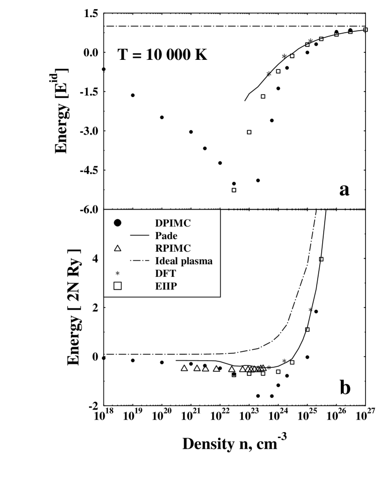
FIG. 1.: Internal Energy of hydrogen for $T=10,000K$, a) normalized to the energy of a noninteracting electron-proton system and b) in units of 2N Rydberg. The curves show results of PACH-calculations (“Pade”), the EIIP model, our Monte Carlo simulations (“DPIMC”), density functional theory (“DFT”) [43] and restricted PIMC data (“RPIMC”) of Militzer et al. [33].

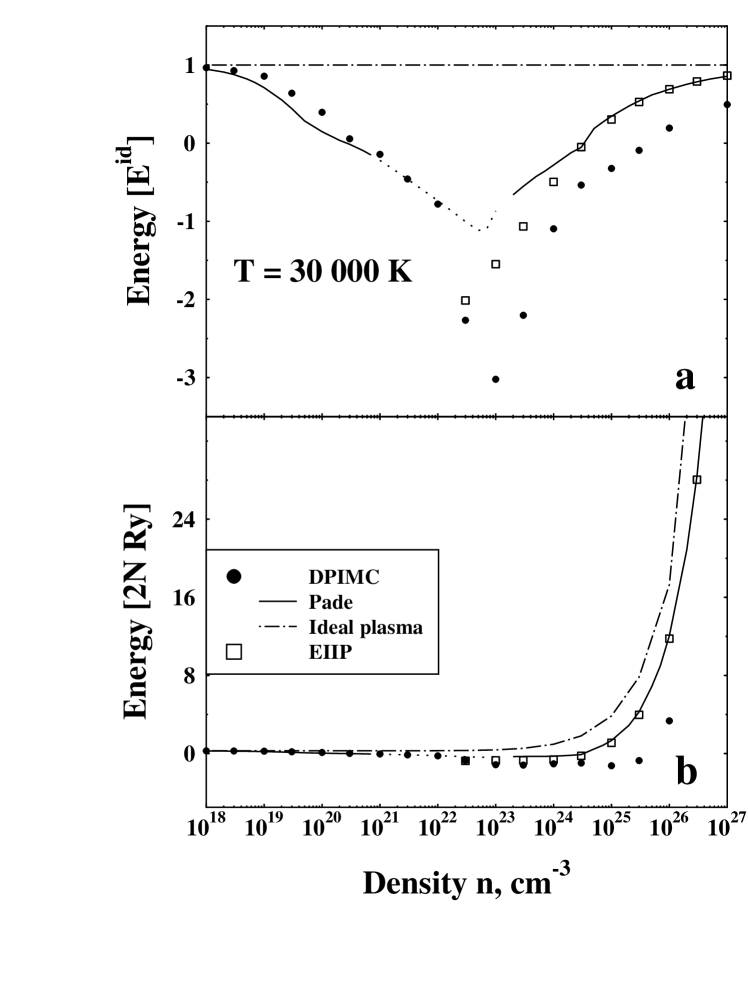
FIG. 2.: Internal Energy of hydrogen for $T=30,000K$. Same notation as in Fig. 1. Dotted line indicates region of low degree of ionization where the Pade and EEIP results are less reliable.

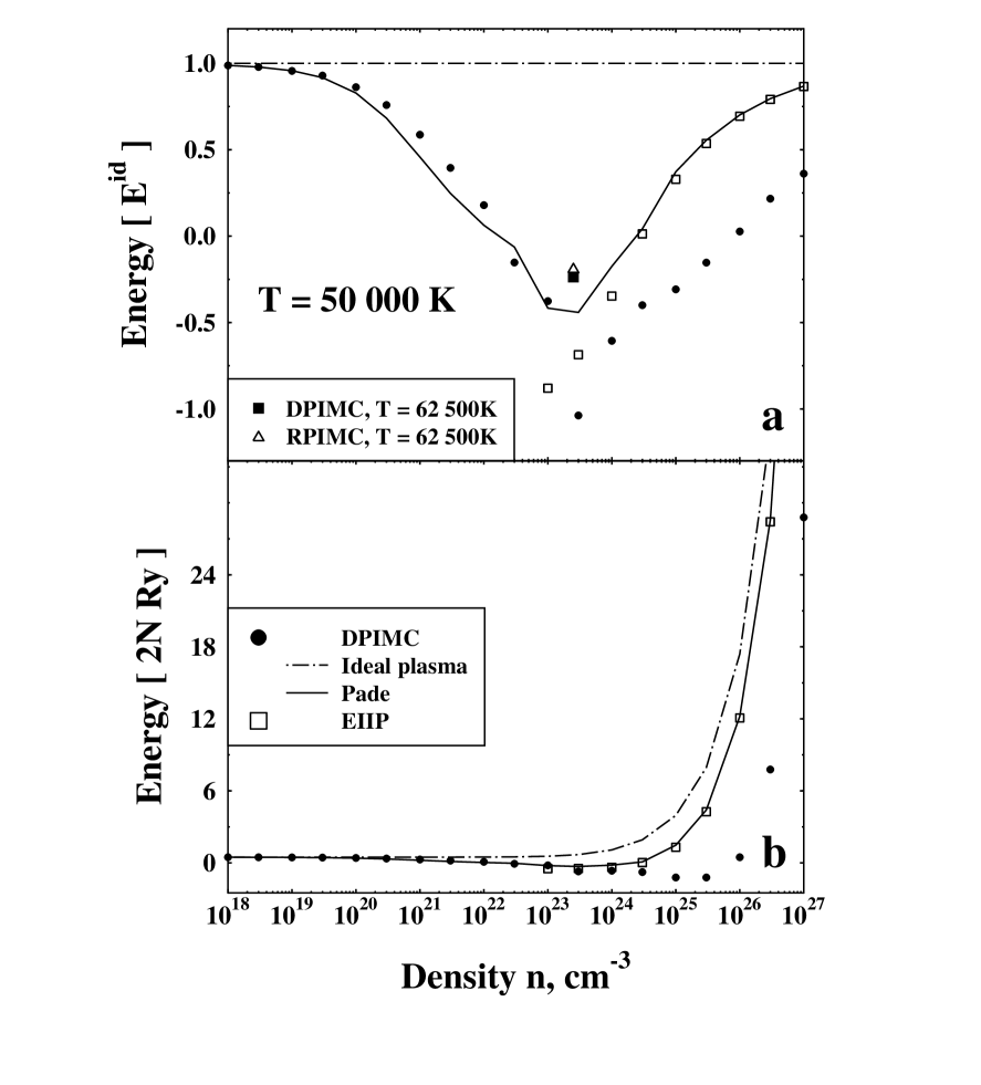
FIG. 3.: Internal Energy of hydrogen for $T=50,000K$. Same notation as in Fig. 1.

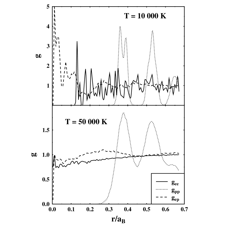
FIG. 4.: Electron-electron (ee), proton-proton (pp) and electron-proton (ep) pair distribution functions of hydrogen from the PIMC simulations at $n=10^{26}$cm^-3 for a temperature of 10,000K (upper figure) and 50,000K (lower figure). Note the different vertical scales.

REFERENCES

- [1] Strongly Coupled Coulomb Systems, G. Kalman (ed.), Pergamon Press 1998
- [2] Proceedings of the International Conference on Strongly Coupled Plasmas, W.D. Kraeft and M. Schlanges (eds.), World Scientific, Singapore 1996
- [3] W.D. Kraeft, D. Kremp, W. Ebeling, and G. Röpke, Quantum Statistics of Charged Particle Systems, Akademie-Verlag Berlin 1986
- [4] M. Bonitz, “Quantum Kinetic Theory”, B.G. Teubner, Stuttgart/Leipzig 1998
- [5] H. Haberland, M. Schlanges, W. Ebeling (eds.): Proc. 10th Int. Workshop on the Physics of Nonideal Plasmas, Contrib. Plasma Phys. 41, No 2-3 (2001).
- [6] L.B. Da Silva et al., Phys. Rev. Lett. 78, 483 (1997).
- [7] S.T. Weir, A.C. Mitchell, and W.J. Nellis, Phys. Rev. Lett. 76, 1860 (1996)
- [8] E.P. Wigner, and H.B. Huntington, J. Chem. Phys. 3, 764 (1935).
- [9] A.A. Abrikossov, JETP (Sov.Phys. - JETP), 39, 1798 (1960); 41, 565 (1961); 45, 2038 (1962).
- [10] N.W. Ashcroft, and D. Stroud, in Solid State Physics, ed. by H. Ehrenreich, F. Seitz, and D. Turnbull (Academic N.Y.), v. 33, p.1. N.W.Ashcroft, Phys.Rev.Lett. 21, 1748 (1968).
- [11] E.G. Brovman, Yu. Kagan, and A. Kholas, JETP (Sov.Phys. - JETP) 61, 2429 (1971).
- [12] G.E. Norman, and A.N. Starostin, Teplofiz. Vys. Temp. 6, 410 (1968); 8, 413 (1970), [Sov. Phys. High Temp. 6, 394 (1968); 8, 381 (1970)]
- [13] P. Haronska, D. Kremp, and M. Schlanges, Wiss. Z. Universität Rostock 98, 1 (1987)
- [14] D. Saumon, and G. Chabrier, Phys. Rev. A 44, 5122 (1991)
- [15] M. Schlanges, M. Bonitz, and A. Tschttschjan, Contrib. Plasma Phys. 35, 109 (1995)
- [16] W. Ebeling, W.D. Kraeft, and D. Kremp, “Theory of bound states and ionization equilibrium in plasmas and solids”. Akademie-Verlag Berlin 1976; Russ. Transl. Mir Moscow 1979
- [17] W. Ebeling, Physica 130 A, 587 (1985)
- [18] W. Ebeling, and W. Richert, Phys. Lett. A 108, 80 (1985); phys. stat sol. (b) 128, 167 (1985).
- [19] D. Beule et al., Phys. Rev. B 59, 14177 (1999 ); Contr. Plasma Phys. 39, 21 (1999)
- [20] V.M. Zamalin, G.E. Norman, and V.S. Filinov, The Monte Carlo Method in Statistical Thermodynamics, (Nauka, Moscow) 1977 (in Russian).
-
[21]
J.-P.Hansen, P.Viellefosse, Phys. Lett. A, 53, 187 (1975);
S. Galam, J.P. Hansen, Phys. Rev. A 14, 816 (1976) - [22] H.E.De Witt, in Strongly Coupled Plasmas, ed. G.Kalman, and P.Carini (Plenum N.Y.), 1978.
- [23] N.P. Kovalenko, Yu.P. Krasny, and S.A. Trigger Statistical theory of liquid metals, (Nauka, Moscow) 1990 (in Russian)
- [24] M. Bonitz et al., J. Phys. B: Condensed Matter 8, 6057 (1996)
- [25] V. Golubnychiy, M. Bonitz, D. Kremp, and M. Schlanges, Phys. Rev. E 64, 016409 (2001).
- [26] W. Ebeling, W. Stolzmann, A. Förster, and M. Kasch, Contr. Plasma Phys. 39, 287 (1999).
- [27] D. Klakow, C. Toepffer, and P.-G. Reinhard, Phys. Lett. A 192, 55 (1994); J. Chem. Phys. 101, 10766 (1994).
- [28] The Monte Carlo and Molecular Dynamics of Condensed Matter Systems, K. Binder and G. Cicotti (eds.), SIF, Bologna 1996
- [29] Classical and Quantum Dynamics of Condensed Phase Simulation, B.J. Berne, G. Ciccotti and D.F. Coker eds., World Scientific, Singapore 1998.
- [30] D.M. Ceperley, in Ref. [28], pp. 447-482
- [31] D.M. Ceperley, Rev. Mod. Phys. 65, 279 (1995)
- [32] B. Militzer, and E.L. Pollock, Phys. Rev. E 61, 3470 (2000)
- [33] B. Militzer, and D.M. Ceperley, Phys. Rev. Lett. 85, 1890 (2000)
- [34] V.S. Filinov, J. Phys. A 34, 1665 (2001).
- [35] V.S. Filinov, P.R. Levashov, V.E. Fortov, and M. Bonitz, in Ref. [67] p. 513, (archive: cond-mat/9912055)
- [36] V.S. Filinov, and M. Bonitz, (archive: cond-mat/9912049)
- [37] V.S. Filinov, M. Bonitz, and V.E. Fortov, JETP Letters 72, 245 (2000)
- [38] V.S. Filinov, V.E. Fortov, M. Bonitz, and D. Kremp, Phys. Lett. A 274, 228 (2000)
- [39] V.S. Filinov, M. Bonitz, W. Ebeling, and V.E. Fortov, Plasma Phys. Contr. Fusion 43, 743 (2001)
- [40] W. Ebeling, Ann. Physik (Leipzig) 21, 315 (1968); 22, 33, 383, 392 (1969); Physica 38, 378 (1968); 40, 290 (1968).
- [41] W. Ebeling, Contr. Plasma Physics 29, 165 (1989); 30, 553 (1990).
- [42] W. Ebeling, A. Förster, V. Fortov, V. Gryaznov, and A. Polishchuk, Thermophysical properties of hot dense plasmas, Teubner, Stuttgart-Leipzig 1991
- [43] H. Xu, and J. P. Hansen, Phys. Rev. E 57, 211 (1998).
- [44] F.J. Dyson, and A. Lenard, J. Math. Phys. 8, 423 (1967)
- [45] E.H. Lieb, and W. Thirring, Phys. Rev. Lett. 31, 111 (1975)
- [46] W.A. Harrison, “Pseudopotentials in the theory of metals”, W.A. Benjamin, INC., New York/Amsterdam 1966.
- [47] V.B. Bobrov, and S.A. Trigger, Solid State Communications 56, 21 and 27 (1985).
- [48] S.D. Kaim, N.P. Kovalenko, and E.V. Vasiliu, J. Phys. Studies 1, 589 (1977).
- [49] G. Mahan, “Many-Particle Physics”, Plenum Press, New York 1981.
- [50] S. Hamaguchi, R.T. Farouki, and D.H.E. Dubin, Phys.Rev. E 56, 4671 (1997)
- [51] R.T. Farouki, and S. Hamaguchi, J. Chem. Phys.101, 9885 (1994).
- [52] W. Ebeling, W.D. Kraeft, D. Kremp, G. Röpke, Physica 140 A, 160 (1986).
- [53] W.L. Slattery, G.D. Doolen, H.E. De Witt, Phys. Rev. A 21, 2087 (1980)
- [54] T. Kahlbaum, in Physics of Strongly Coupled Plasmas, W.D. Kraeft, M. Schlanges (eds.), World Scientific, Singapore 1996
- [55] R.P. Feynman, and A.R. Hibbs, Quantum mechanics and path integrals, McGraw-Hill, New York 1965
- [56] V.S. Filinov, High Temperature 13, 1065 (1975) and 14, 225 (1976)
- [57] B.V. Zelener, G.E. Norman, V.S. Filinov, High Temperature 13, 650, (1975)
- [58] G. Kelbg, Ann. Physik, 12, 219 (1963); 13, 354; 14, 394 (1964).
- [59] W. Ebeling, H.J. Hoffmann, and G. Kelbg, Contr. Plasma Phys. 7, 233 (1967) and references therein.
- [60] A.V. Filinov, Yu.E. Lozovik, and M. Bonitz, phys. stat. sol. (b), 221, 231 (2000)
- [61] A.V. Filinov, M. Bonitz, and Yu.E. Lozovik, Phys. Rev. Lett. 86, 3851 (2001)
- [62] S.A. Trigger, and W. Ebeling, Proceedings of the IInd Capri Workshop on Dusty Plasmas, Capri, May 2001, in print.
- [63] N.I. Klyuchnikov, and S.A. Trigger, Doklady of Russian Academy of Science (Sov.Phys - Doklady) 238, 565 (1978) (in Russian).
- [64] V.S. Filinov, V.E. Fortov, M. Bonitz, and P.R. Levashov, accepted for publication in JETPL
- [65] Using a modified PACH approach, Beule et al. [19] predicted a first order phase transition in hydrogen for K with a pressure and density GPa and gcm-3. Similar results were obtained by Schlanges et al. [15].
- [66] In fact, the first minimum of the proton-proton function (around ) for K is far lower than the standard value of 0.35 typical for a liquid.
- [67] “Progress in Nonequilibrium Greens Functions”, M. Bonitz (ed.), World Scientific Publ., Singapore 2000.