Alteration of Chemical Concentrations through Discreteness-Induced Transitions in Small Autocatalytic Systems

Abstract

We study an autocatalytic system consisting of several interacting chemical species. We observe a strong dependence of the concentrations of the chemicals on the size of the system. This dependence is caused by the discrete nature of the molecular concentrations. Two basic mechanisms responsible for them are identified and elucidated. The relevance of the transitions to processes in biochemical systems and in micro-reactors is briefly discussed.

Keywords: Discreteness, Phase Transition, Stochastic Processes, Reactions, Biochemical Systems

Rate equations are often employed in the study of biochemical reaction processes. In rate equations, the quantities of chemicals are treated as continuous variables, and the actual discreteness of the molecular concentration is ignored. Of course, fluctuations of numbers of molecules have been studied using stochastic differential equations and introduced non-trivial effects [1, 2]. Still, discreteness has not been considered in any such study. In many biochemical processes, however, some chemicals play important roles at extremely low concentrations, amounting to only a few molecules per cell [3, 4]. Furthermore, there exist amplification mechanisms involving enzymes in cells through which even a change by one molecule in a cell can result in drastic effects. In such situations, the discreteness of the molecular concentration is obviously not negligible.

We previously showed the existence of a novel transition induced by the discreteness of the molecular concentration in an autocatalytic reaction system [5]. The system contains four chemicals $X_{i}(i=1,\cdots,4)$. We considered an autocatalytic reaction network (loop) represented by $X_{i}+X_{i+1}\rightarrow 2X_{i+1}$ (with $X_{5}\equiv X_{1}$) within a container that is in contact with a reservoir of molecules. Through interaction with the reservoir, each molecule species $X_{i}$ diffuses in and out at a total rate of $D_{i}s_{i}V$, where $D_{i}$ is the flow rate, $s_{i}$ the concentration of chemical $X_{i}$ in the reservoir, and $V$ the volume of the container. In this system, a novel state appears as a result of fluctuations and the discreteness of the molecular concentration, characterized as extinction and subsequent reemergence of molecule species alternately in the autocatalytic reaction loop.

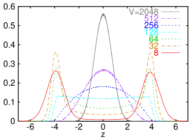
Figure 1: Probability distribution of $z\equiv(x_{1}+x_{3})-(x_{2}+x_{4})$. Here $s_{i}=1$, and $D=1/128$. For $V\geq 256$, $z$ has a distribution around $0$, corresponding to the fixed point state $x_{i}=1$ (for all $i$). For $V\leq 64$, the distribution has double peaks around $z=4$, corresponding to the 1-3 rich state ($N_{1},N_{3}\gg N_{2},N_{4}\approx 0$), and $z=-4$, corresponding to the 2-4 rich state.

When the volume of the container is small, $N_{i}$, the number of molecules of species $X_{i}$, may go to $0$ (i.e. become extinct) through a finite-size fluctuation due to the discreteness of the molecular concentration. Once $N_{i}$ reaches $0$, it remains $0$ until an $X_{i}$ molecule flows in. Thus, if the flow rate of molecules is sufficiently small, state with $N_{1}=N_{3}=0$ or $N_{2}=N_{4}=0$ can be realized. In a state with $N_{2},N_{4}\approx 0$ (a “1-3 rich” state), switches between states with $N_{1}>N_{3}$ and $N_{3}>N_{1}$ can occur, and similarly for a state with $N_{1},N_{3}\approx 0$ (a “2-4 rich” state). A symmetry-breaking transition to these states was observed in our previous study, with the decrease of $V$, as is shown in Fig. 1, as the change of the probability distribution of the number of molecules. For large $V$, corresponding to the continuum limit, the distribution of $z=((N_{1}+N_{3})-(N_{2}+N_{4}))$ shows a single-peaked distribution around $z=0$, whereas it is replaced by a symmetric, double-peak distribution as $V$ is decreased. This is a novel discreteness-induced transition (DIT) occurring with the decrease of $V$. The transition occurs without any change of parameters, and thus cannot be discussed in the rate equation with noise (i.e., by the continuum description).

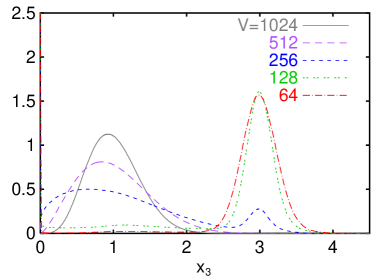
Figure 2: Probability distribution of $x_{3}$ in our model with $s_{1}=s_{2}=1.99$, $s_{3}=s_{4}=0.01$, $D=1/128$, sampled over a time span of $5\times 10^{6}$, for different $V$ (see Case II for details).

In the system investigated in our previous work, the long-term average concentration of each chemical does not differ from that in the continuum limit, since the system over time switches between the two states of broken symmetry. It is important to determine if there are systems for which the average concentrations of chemicals are significantly altered by the DIT. We will show that this is possible in a system possessing some kind of asymmetry. With the DIT without symmetry breaking, the average concentrations of chemicals are drastically altered by the change of $V$. The peak position of the distribution is changed with a finite jump, as the volume is decreased (see Fig. 2, while see later sections for the description of the model and simulation). Borrowing the term of thermodynamics, the DIT reported previously is regarded as a second order transition involving symmetry breaking, while the DIT reported here corresponds to the first order transition without symmetry breaking. This result is biologically significant as providing a possible description of the alteration of the concentrations of some molecules within cells. Note in a cell, the number of molecules of each chemical species is not necessarily huge, and the discreteness effect is not always negligible.

To investigate this problem, we again use an autocatalytic reaction loop of chemicals, but here we consider the case in which $D_{i}$, $r_{i}$ or $s_{i}$ is dependent on the chemical species $i$, where $r_{i}$ is the reaction constant of the reaction $X_{i}+X_{i+1}\rightarrow 2X_{i+1}$. To study the effects of discreteness, we investigated the reaction model by using a stochastic particle simulation. We assumed that the chemicals are well stirred in the container. At each simulation step, two molecules in the container are randomly chosen. Then we judge if the molecules react or not, by checking if one of the two acts as a catalyst for the other as a substrate. To carry out the simulation efficiently here, we adopted Gillespie’s direct method [6] (see Appendix) [7].

Note that for there to be a DIT to a 1-3 or 2-4 rich state, it is necessary that the time interval for inflow of molecules be longer than the time scale of the reactions. This time interval for $X_{i}$ inflow should be $\sim 1/D_{i}s_{i}V$. In our previous study, in which we considered the case of identical parameter values for all $i$, the discreteness of the molecular concentration has the same effect for all the molecule species, and the transition occurs near $DsV=r$.

It is important to realize that the relevance of the discreteness of the molecular concentration depends on the reaction and flow rates of each molecule when the parameter values are not identical. For example, if $D_{1}s_{1}<D_{2}s_{2}$, the inflow time interval for $X_{1}$ molecules is longer than that for $X_{2}$ molecules, so that the discreteness of the $X_{1}$ flow has a greater effect on the behavior of the system. In general, $V$ may determine the species that become extinct, and the average concentration of each molecule can be greatly changed by the discreteness effect.

Here, we consider the case in which $s_{i}$ is species dependent, while $D$ and $r$ are identical for all species, for the autocatalytic loop introduced above. With this choice, the discreteness effect of each chemical $X_{i}$ depends on $i$. In this system, we find discreteness effects that result in changes of the average concentrations $\bar{x_{i}}$, with the temporal average of the concentration $x_{i}=N_{i}/V$. Although this result is obtained with this simple example, the mechanism we find would appear to be quite general, and hence there is reason to believe that the DIT we find exists in a wide variety of real systems.

We first consider the effect of the discreteness of the inflow of chemicals and how this depends on the relation between the reaction rate and the inflow rate. In our model, the inflow interval of $X_{i}$ is $\sim\frac{1}{Ds_{i}V}$, and the time scale of the reaction is $\sim\frac{x_{i}}{rx_{i}x_{i+1}}$. When the former time scale is larger than the latter, the reaction from $i$ to $i+1$ can proceed to completion before the inflow of species $i$ occurs. Then $N_{i}$ becomes $0$. As long as $N_{i}=0$, no reaction to produce chemical $X_{i}$ occurs, and the average density may be decreased radically from the continuum limit case.

Case I : inflow discreteness and reaction rate

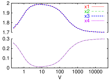
Figure 3: The average concentration $\bar{x_{i}}$ in Case I : $s_{1}=s_{3}=1.7$, $s_{2}=s_{4}=0.3$, as a function of the volume $V$ (sampled over a time span of $10^{6}$ for $V>1024$, $10^{7}$ for $32<V\leq 1024$, and $10^{8}$ for $V\leq 32$, also the same for Figs. 5 and 9). $D=1/128$.

As a simplest example to study this mechanism, we consider the case with $s_{1}=s_{3}>s_{2}=s_{4}$. In this case, the rate equation in the continuum limit has a stable fixed point $\forall i:x_{i}=s_{i}$. When $V$ is large, each $x_{i}$ fluctuates around this fixed point. The average concentration $\bar{x_{i}}$ is shown in Fig. 3. With the decrease of $V$, the difference between the pair $\bar{x_{1}}$ and $\bar{x_{3}}$ and the pair $\bar{x_{2}}$ and $\bar{x_{4}}$ is amplified, and there is clear deviation from the continuum limit case.

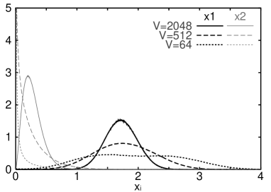
Figure 4: Probability distribution of $x_{1}$ and $x_{2}$, sampled over a time span of $5\times 10^{6}$. $s_{1}=s_{3}=1.7$, $s_{2}=s_{4}=0.3$ (Case I). $D=1/128$. In the case $V=2048$, peaks around $x_{i}=s_{i}$, which correspond to the fixed point at the continuum limit, is shown. As $V$ decreases, the peaks get broader according to fluctuations, and the tail of the distribution of $x_{2}$ reaches $0$. Thus, there appears a peak around $x_{2}=0$.

The mechanism responsible for this amplification can be understood as follows. As $V$ is decreased, we have found that the 1-3 rich state, with extinction of $N_{2}$ and $N_{4}$, appears when the increase of $\bar{x_{1}}$ and $\bar{x_{3}}$ occurs. To realize $N_{2}=N_{4}=0$, it is necessary for the inflow interval of $X_{2}$ or $X_{4}$ to be longer than the time scale of the reaction. The inflow interval of $X_{i}$ molecules is $\sim\frac{1}{Ds_{i}V}$, while the time scale for the reaction is $\sim\frac{x_{i}}{rx_{i}x_{i+1}}$. Since we set $r=1$ and $x_{i}=O(1)$, the 1-3 rich state appears for $\frac{1}{Ds_{2}V},\frac{1}{Ds_{4}V}>\frac{1}{r}$, while the 2-4 rich state appears for $\frac{1}{Ds_{1}V},\frac{1}{Ds_{3}V}>\frac{1}{r}$. Thus in the present case, the 1-3 rich state is first observed as $V$ is decreased. In the range of values of $V$ for which the relations $\frac{1}{Ds_{1}V},\frac{1}{Ds_{3}V}<\frac{1}{r}<\frac{1}{Ds_{2}V},\frac{1}{Ds_{4}V}$ are satisfied, the 1-3 rich state is realized often, while the 2-4 rich state is not (see Fig. 4).

Once the 1-3 rich state is realized, an $X_{2}$ molecule and an $X_{4}$ molecule must enter the system almost simultaneously for the system to break out of this state. Thus the ‘rate of interruption’ of the 1-3 rich state is roughly proportional to $s_{2}s_{4}V^{2}$, the product of the rates of $X_{2}$ inflow and $X_{4}$ inflow. The expected residence time in the 1-3 rich state is the reciprocal of the rate of interruption. Thus the ratio of the expected residence times in the 1-3 rich and 2-4 rich states is $\frac{s_{1}s_{3}}{s_{2}s_{4}}$.

From the above considerations, we expect that for some $V\approx\frac{r}{Ds_{2}}$, there appears a transition to the 1-3 rich state, leading to a drastic increase of the 1-3 concentration. The validity of this conclusion has been confirmed by several simulations, one of whose results is shown in Fig. 3.

Case I^′ : imbalance of inflow discreteness

The transition discussed above can create a stronger effect on the concentrations. As an example, consider the case $s_{1}=s_{3}>s_{2}>s_{4}$.

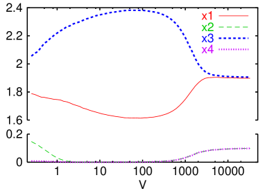
Figure 5: The average concentration $\bar{x_{i}}$ in Case I^′ : $s_{1}=s_{3}=1.9$, $s_{2}=0.19$, $s_{4}=0.01$, as a function of the volume $V$. $D=1/128$.

In this case, as in case I, the 1-3 rich state is stable. While in this state, the system switches from a condition of $N_{1}>N_{3}$ to one of $N_{1}<N_{3}$ due to $X_{2}$ inflow and from $N_{1}<N_{3}$ to $N_{1}>N_{3}$ due to $X_{4}$ inflow. Since the latter event is less frequent for $s_{2}>s_{4}$, the condition $N_{1}<N_{3}$ is satisfied for a greater amount of time in the 1-3 rich state. Hence, it is expected that $\bar{x_{1}}<\bar{x_{3}}$. This is confirmed by the results displayed in Fig. 5. This is in strong contrast with the result in the continuum limit, where $\bar{x_{1}}\approx\bar{x_{3}}$ if $D\ll rs_{i}$ (i.e., the time scale of the reactions is much shorter than that of the inflow). The significant difference between $\bar{x_{1}}$ and $\bar{x_{3}}$ found here appears only when the 1-3 rich state is realized through the effect of the discreteness of the flow of $X_{4}$ molecules. As shown in Fig. 5, there is amplification of the difference between $\bar{x_{1}}$ and $\bar{x_{3}}$ as $V$ decreases that occurs simultaneously with the transition to the 1-3 rich state.

Case II : inflow and outflow

When $Ds_{i}V$ is small enough to insure the existence of both 1-3 and 2-4 rich states, the preference of states can depend on the concentrations $s_{i}$. The preferred state is selected through another DIT caused by outflow rather than inflow of a particular chemical.

As an example, we consider the case $s_{2}\geq s_{1}>s_{3}=s_{4}$. Here again, the rate equation in the continuum limit has a stable fixed point. If $D\ll rs_{i}$, then $x_{1},x_{3}\approx\frac{s_{1}+s_{3}}{2}$ and $x_{2},x_{4}\approx\frac{s_{2}+s_{4}}{2}$ at the fixed point.

As discussed above, 1-3 and 2-4 rich states appear for small $Ds_{3}V$. In the 2-4 rich state, it is likely for $N_{4}$ to decrease as a result of the outflow of $X_{4}$ and the reaction $X_{4}+X_{1}\rightarrow 2X_{1}$ facilitated by the inflow of $X_{1}$.

If $s_{4}V<1$, it may be the case that all $X_{4}$ molecules flow out, and $N_{4}$ becomes $0$. The time required to realize $N_{4}=0$ from $N_{4}=n$ should be $\sim\frac{1}{D}\log n$ when $s_{4}V\approx 0$ and $n\gg 1$. However, if $s_{1}$ is large, $X_{4}$ will be consumed by the reaction caused by $X_{1}$, and for this reason, $N_{4}$ will decrease to $0$ more rapidly. The time required to use up $X_{4}$ may also depend on $s_{1}$. In this case, the 1-3 rich state is favoured by the mechanism described below.

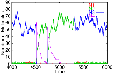
Figure 6: Time series of the number of molecules $N_{i}$ for $V=16$. Here $s_{1}=0.09$, $s_{2}=3.89$, $s_{3}=s_{4}=0.01$, and $D=1/64$. There is a transition to the 2-4 rich state at $t=4511$. In the 2-4 rich state, $X_{4}$ molecules flow out at the rate $D$, and $N_{4}$ thereby decreases. Due to the flow of $X_{3}$ molecules, switching from $N_{2}>N_{4}$ to $N_{2}<N_{4}$ occurs, and $N_{4}$ increases again (as seen at $t=4743$). Here, the interval over which the switching takes place is longer than the interval of $X_{3}$ inflow, $1/DVs_{3}=400$, and is indeed long enough for most $X_{4}$ molecules to diffuse out before $X_{3}$ molecules can flow into the system. Thus, here $N_{4}$ readily decreases to $0$ before the switch. At $t=5300$, with $N_{4}=0$ an $X_{3}$ molecule flows into the container, leading to a switch to the 1-3 rich state.

When $N_{4}>0$, $N_{4}$ can increase again as a result of $X_{3}$ inflow, which leads to switch from the $N_{2}>N_{4}$ condition to the $N_{2}<N_{4}$ condition. The inflow interval for $X_{3}$ is $\sim\frac{1}{Ds_{3}V}$. If this interval is much shorter than the time required for $N_{4}$ to reach $0$, $N_{4}$ may increase again, causing the 2-4 rich state to be preserved. However, if the interval is longer, $N_{4}$ may decrease to $0$, in which case, the 2-4 rich state can be readily destroyed by the inflow of an $X_{3}$ molecule, as shown in Fig. 6.

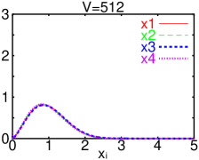
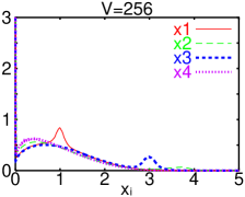
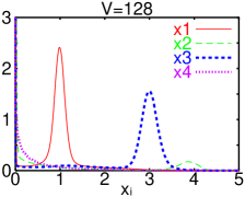
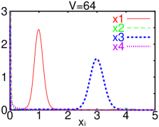
Figure 7: Probability distribution of $x_{i}$ in Case II : $s_{1}=s_{2}=1.99$, $s_{3}=s_{4}=0.01$, sampled over a time span of $5\times 10^{6}$, for different $V$. $D=1/128$. In the case $V=512$, all $x_{i}$ shows peaks around $x_{i}=1$, which correspond to the fixed point at the continuum limit. When $V$ is small, each $x_{i}$ shows a peak at a different concentration, and the peak height changes greatly with change of $V$. For $V=256$, there appear peaks at around $x_{1}=1$, $x_{3}=3$, $x_{2}=4$, and also around $x_{i}=0$ (for all $i$). With further decrease of $V$, $N_{2}$ and $N_{4}$ reach $0$ more easily than $N_{1}$ and $N_{3}$ do. Accordingly the peaks for $x_{2}$ and $x_{4}$ around 0 grows as shown in the case $V=128$. The system tends to stay at the 1-3 rich state, and the peak around $x_{2}=4$ gets smaller (as shown in the case $V=64$).

When the system is in the 1-3 rich state, on the other hand, switches from a condition of $N_{1}>N_{3}$ to one of $N_{1}<N_{3}$ due to $X_{2}$ inflow, cause $N_{3}$ to remain large (as in case I^′). The system therefore tends to maintain the condition $N_{1}<N_{3}$ (as long as $D/rs_{i}$ is not too large). However, $N_{1}$ only rarely decreases to $0$, unlike $N_{4}$, because $s_{1}$ is relatively large. Thus the 1-3 rich state is more stable than the 2-4 rich state, as shown in Figs. 7 and 8.

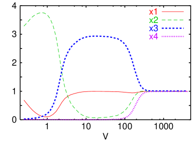
Figure 9: The average concentration $\bar{x_{i}}$ in Case II : $s_{1}=s_{2}=1.99$, $s_{3}=s_{4}=0.01$, as a function of the volume $V$. $D=1/128$.

Hence, when $V$ is decreased sufficiently to satisfy $s_{4}V<1$, and the time interval $\frac{1}{Ds_{3}V}$ is sufficiently long to allow $N_{4}$ to decrease to $0$, the 2-4 rich state loses stability, and the residence time in the 1-3 rich state increases, due to the discreteness of $X_{4}$. As a consequence, $\bar{x_{3}}$ increases as $V$ decreases, as shown in Fig. 9.

Amplification by Discreteness

Summarizing the findings discussed above, differences among the ‘degrees of discreteness’ of the chemicals lead to novel DIT. The average chemical concentrations are greatly altered by this DIT. Indeed, as the system size (the volume $V$) changes, there is a sharp transition to a state qualitatively different from that found in the continuum limit. There are two key parameters with regard to discreteness: One is $\frac{1}{Ds_{i}V}$ (investigated in case I), the inflow time interval for $X_{i}$, and the other is $s_{i}V$ (investigated in case II), the number of species $X_{i}$ molecules in the system when it is at equilibrium with the reservoir.

If the interval $\frac{1}{Ds_{i}V}$ is longer than the time scale of the reaction, $\frac{x_{i}}{rx_{i}x_{i+1}}$, the discreteness of the $X_{i}$ inflow is relevant. In such a situation, the $X_{i}$ molecules present in the system may be completely consumed by the reaction before any new $X_{i}$ molecules flow in, so that $N_{i}$ may reach $0$.

Then, if the condition $s_{i}V<1$ is satisfied in addition to the above stated condition, $N_{i}$ can become $0$ as a result of all $X_{i}$ molecules flowing out of the system. In this case, the relation between the time necessary to realize a switch that increases $N_{i}$ and the time necessary for $N_{i}$ to decay to $0$ is also important.

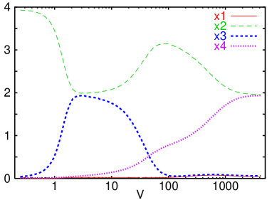
Figure 10: The average concentrations $\bar{x_{i}}$, sampled over a time span of $5\times 10^{8}$ for $V\leq 32$ and $5\times 10^{6}$ for $V>32$, plotted as functions of the volume $V$. $s_{1}=0.09$, $s_{2}=3.89$, $s_{3}=s_{4}=0.01$, $D=1/64$. For large $V$, $\bar{x_{i}}$ is close to the fixed point value of the continuum limit. As $V$ decreases, there first appears a 2-4 rich state, but for smaller $V$, this 2-4 rich state becomes unstable, and the residence time of the 1-3 rich state increases, leading to a sharp increase of $\bar{x_{3}}$. For much smaller $V$ ($<0.5$), only $X_{2}$ molecules exist for most of the time.

With the above two conditions satisfied for each species $X_{i}$, there appear several switches to different states as $V$ is changed. As an example, we considered the case in which $s_{1}=0.09$, $s_{2}=3.89$, $s_{3}=s_{4}=0.01$, and $D=1/64$. In this case, the average concentration $\bar{x_{i}}$ exhibits three transitions as $V$ is decreased, as shown in Fig. 10.

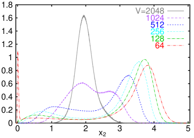
Figure 11: Probability distribution of $x_{2}$, sampled over a time span of $5\times 10^{6}$. $s_{1}=0.09$, $s_{2}=3.89$, $s_{3}=s_{4}=0.01$, and $D=1/64$. When $V$ is large, there is a single peak around $x_{2}=2$, which corresponds to the fixed point in the continuum limit. Around $V=10^{3}$, double peaks appear around $x_{2}=1$ and $x_{2}=3$, corresponding to the 2-4 rich state. As $V$ decreases, these two peaks move apart, and near $V=10^{2}$, the tail of the lower peak reaches $0$, implying that $N_{2}$ and $N_{4}$ often decrease to $0$. Thus here, the 2-4 rich state is unstable. Then, as $V$ is decreased further, the peak at $x_{2}=0$ rises sharply.

First, in the continuum limit, $\bar{x_{1}}$ and $\bar{x_{3}}$ are very small, as resulted from the fact that $s_{1}+s_{3}\ll s_{2}+s_{4}$. Around $V=10^{3}$, the discreteness of $X_{3}$ becomes significant, and the 2-4 rich state appears. Then the reactions $X_{2}+X_{3}\rightarrow 2X_{3}$ and $X_{3}+X_{4}\rightarrow 2X_{4}$ take place only sporadically. Contrastingly, the flow of $X_{1}$ molecules is fairly steady. Thus, while the system is in the 2-4 rich state, $N_{2}>N_{4}$ is satisfied for most of the time, as shown in case I^′. Figure 11 displays the distribution of $x_{2}$. Double peaks corresponding to the 2-4 rich state appear in this situation.

In the 2-4 rich state with $N_{2}>N_{4}$, $X_{2}$ molecules flowing into the system raise $N_{2}$ to the level of $s_{2}V$, establishing equilibrium with the reservoir. At the same time, $X_{4}$ molecules flow out, and $N_{4}$ decreases to the level of $s_{4}V$, as seen in case II.

As seen in case II, The difference between $N_{2}$ and $N_{4}$ increases with further decrease of $V$, since the switching rate decreases. In Fig. 11, the gap between the two peaks in the distribution of $X_{2}$ is seen to become larger as $V$ decreases. Around $V=10^{2}$, finally, the imbalance between $N_{2}$ and $N_{4}$ destabilizes the 2-4 rich state. For this reason, the 1-3 rich state becomes almost as stable as (or more stable than) the 2-4 rich state, in spite of the relation $s_{1}+s_{3}\ll s_{2}+s_{4}$. The residence time in the 1-3 rich state increases sharply, causing $\bar{x_{3}}$ to increase (as shown in Figs. 6 and 10). In fact, $\bar{x_{3}}$ increases to approximately $2$, which is more than 30 times larger than its value in the continuum limit [8].

For very small $V$ (i.e. $V<2$), $N_{1}$ and $N_{3}$ decrease to $0$ quite readily, and thus the 1-3 rich state is also easily destroyed. In this situation, for most of the time only one chemical exists in the container. Here, only $\bar{x_{2}}$ has a large value, with all of the others near or at $N_{i}=0$.

In the manner described above, non-trivial alteration of chemical concentrations as a result of DIT was observed. It has been found that those molecule species whose numbers vanish are determined not only by the flow rates but also by the network and dynamics of the reactions. For example, when $V$ is relatively large ($V\approx 10^{2}$), $\bar{x_{3}}$ decreases as $s_{3}$ increases.

Discussion

In conclusion, we have reported a DIT that leads to a strong effect on the average concentrations of the chemicals. Although we have studied a simple case with only four chemicals here, we have found that this type of DIT appears in more complex reaction networks of a more general nature.

In fact, we have randomly chosen a catalytic reaction network consisting of few hundred species, and studied the population dynamics of each chemical species with the scheme of stochastic simulation adopted here. For some reaction networks we have observed the DIT as the volume is decreased. In such cases, we have found that the combination of the two mechanisms we studied here leads to a variety of transitions and alterations of molecular concentrations. Although the example reported in the present paper is quite simple and may look special, the mechanism found in the example gives a basis for DIT in complex reaction network.

Generally speaking, DIT and its effects on molecular concentrations are likely to be observed with chemical networks containing autocatalytic reactions. However, in some examples they are observed even without autocatalytic reactions. When some part of reaction networks works as an autocatalytic sub-network as a set, as seen in hypercycles [11], the DIT of the present mechanism is possible.

It is now experimentally feasible to construct a catalytic reaction system in a micro-reactor, and to design other types of systems with small numbers of molecules. Also, there was great advance in techniques for detection of small numbers (on the order of $1$ to $10^{2}$) of molecules using fluorescence or other new methods such as thermal-lens microscopy [12]. In such systems, experimental verification of DIT should be possible. Also, we believe that the alterations of chemical concentrations resulting from DIT that we found will have practical applications, since quite high accumulation of dilute chemical species is possible as we have shown here.

Since the number of molecules in a biological cell is often small, the relevance of DIT to cell biology is obvious. For example, in cell transduction, the number of signal molecules is often less than 100, and even a single molecule can switch the biochemical state of a cell [13]. In our visual system, a single photon in retina is amplified to a macroscopic level [14]. Transmission of signals through neurons via synapses also often involves a small number of molecules [15]. Chemical reaction network consisting of several autocatalytic reaction is widely seen in a cell, and such autocatalytic process provides a candidate for amplification of an effect of a single molecule. Since the DIT we reported here is generally observed in autocatalytic reaction networks, it is expected that it may be used in a biochemical reaction network in a cell. Indeed, according to our results, the non-trivial accumulation of dilute molecules and switching among several distinct states with different chemical compositions may be realizable by, for example, the control of flow by receptor. Additionally, in some preliminary simulations with large reaction networks, some sub-networks can be effectively activated or inactivated by DIT. In such cases, transitions between several states characterized by active sub-networks can be observed, which will be relevant to switching between cellular states by a few signal molecules.

Switching the expression of genes on and off is a focus of interest in bioinformatics. This digital behavior is also connected with the concentration of proteins present. As is pointed out [13], genetic regulation is under stochasticity coming from smallness in the number of associated molecules. As we have seen in our model, one chemical species can exhibit both an on/off switch and continuous regulation of other chemicals, even if the number of molecules of this species is small. We believe that the switching of chemical states facilitated by our DIT plays a role in the regulation of genetic and metabolic processes in cells.

Throughout the paper we have adopted stochastic particle simulations. Of course master equation approach is also equivalently possible, which is especially useful if some analytic tools for it are developed. For example, use of Fokker-Planck equations derived in the limit of large volume (molecule numbers), is a powerful tool [16]. Since our DIT occurs when the volume (the number of molecules) is quite small, such tools are so far not available. In future it will also be important to develop some analytic tools for a system where the discreteness in the number is essential.

Acknowledgements

This research was supported by Grants-in-Aid for Scientific Research from the Ministry of Education, Culture, Sports, Science and Technology of Japan (11CE2006).

Appendix : Details of the Simulation

Details of the Model

We assumed that the chemicals are well stirred in the container and the molecules have no volume. Thus the rate of the reaction $X_{i}+X_{i+1}\rightarrow 2X_{i+1}$ is given by $R_{i}\equiv r_{i}x_{i}x_{i+1}$ [concentration / time], where $r_{i}$ is the reaction constant and $x_{i}$ is the concentration of the chemical $X_{i}$. By rewriting it with the use of $N_{i}$, the number of $X_{i}$ molecules, the rate of the reaction is given by $R_{i}V\equiv\frac{r_{i}N_{i}N_{i+1}}{V}$ [reactions / time]. In the same way, the rate of the $X_{i}$ inflow is given by $D_{i}s_{i}V$ [molecules / time], corresponding to $D_{i}s_{i}$ [concentration / time], whereas that of the $X_{i}$ outflow is given by $D_{i}N_{i}$ [molecules / time], corresponding to $D_{i}x_{i}$ [concentration / time].

This stochastic model approaches the rate equation

$$\frac{dx_{i}}{dt}=r_{i-1}x_{i-1}x_{i}-r_{i}x_{i}x_{i+1}+D_{i}(s_{i}-x_{i})$$

when one takes a continuum limit, given by $V\rightarrow\infty$.

We also assumed that the area of the surface of the container is proportional to the volume $V$, and thus the rate of the $X_{i}$ flow is proportional to $D_{i}V$, to have this well-defined continuum limit for $V\rightarrow\infty$. One might assume that the area of the surface should be $V^{2/3}$, and the rate of the $X_{i}$ flow should be proportional to $D_{i}V^{2/3}$. This change of setting alters just the parameter values. By suitably adjusting parameters $D_{i}$ and/or $s_{i}$, the same transitions to the switching states and the alteration of average concentrations are observed, even with such settings.

With the rates of the reactions and the flows above, we carried out the stochastic simulation. In principle, one can carry out the simulation, by randomly selecting two molecules, and transforming one of them to other molecule, according to the reaction rule, with the probability proportional to the rate of reaction, when these molecules react. Here, as an efficient simulation method, we adopt Gillespie’s direct method, instead.

Gillespie’s Direct Method

In our system, the state of the system is determined by $N_{i}$, the number of molecules, and is changed only when one reaction or one molecular flow occurs. Thus the rate of the reactions and the flows do not change until the next event (one reaction or one molecular flow) occurs, so that the lapse time to the next event decays exponentially.

Gillespie’s direct method [6] stands on this fact. First, we determine the lapse time to the next event by exponentially-distributed random numbers, and set the time forward. Next, we determine which event occurs, with the proportion to the rate of the event. We change the state according to the event, and re-calculate the rate of the reactions and the flows. These steps are executed repeatedly, until the specified time elapses.

In some cases, especially with complicated reaction networks, there are more efficient methods (see refs. [17, 18]). Here, for simplicity, we adopted the Gillespie’s direct method. Our result discussed above does not depend on which method to use.

Figure 8: Probability distribution of $(x_{1}+x_{3})$ and $(x_{2}+x_{4})$ in Case II : $s_{1}=s_{2}=1.99$, $s_{3}=s_{4}=0.01$, sampled over a time span of $5\times 10^{6}$. $V=32$, $D=1/128$. With such a small $V$, the 2-4 rich states are destabilized, and the rate of the residence at the 1-3 rich states is almost $10^{2}$ times larger than that at the 2-4 rich states. The state allowed by the continuum limit, $x_{1}+x_{3}\approx x_{2}+x_{4}$ is very rare.

References

- [1] W. Horsthemke and R. Lefever: Noise-Induced Transitions, ed. H. Haken (Springer, 1984).
- [2] K. Wiesenfeld and F. Moss: Nature 373 (1995), 33.
- [3] B. Alberts, D. Bray, J. Lewis, M. Raff, K. Roberts and J. D. Watson: The Molecular Biology of the Cell (Garland, New York, 1994) 3rd ed.
- [4] N. Olsson, E. Piek, P. ten Dijke and G. Nilsson: J. Leuko. Biol. 67 (2000), 350.
- [5] Y. Togashi and K. Kaneko: Phys. Rev. Lett. 86 (2001), 2459.
- [6] D. T. Gillespie: J. Phys. Chem. 81 (1977), 2340.
- [7] The choice of this method is only for efficiency. The numerical result by the method agrees with that of the direct simulation, as long as the time resolution and the resolution of the random number generator is sufficient.
- [8] The amplification rate, i.e. the ratio of the maximum , to at the continuum limit, depends on the parameters , , and . At the continuum limit, and , if . When is moderately small and the 1-3 rich states are more stable than the 2-4 rich states, holds, as described already. In this case, because . Thus the maximum value of is around (or more than) half of the total concentration (, if ). Thus, roughly speaking, the amplification rate of is around . For , , , the value is , as is consistent with that shown in Fig. 10.
- [9] B. Hess and A. S. Mikhailov: Science 264 (1994), 223.
- [10] B. Hess and A. S. Mikhailov: J. Theor. Biol. 176 (1995), 181.
- [11] M. Eigen, P. Schuster: The Hypercycle (Springer, 1979).
- [12] K. Sato, H. Kawanishi, M. Tokeshi, T. Kitamori and T. Sawada: Anal. Sci. 15 (1999), 525.
- [13] H. H. McAdams and A. Arkin: Trends Genet. 15 (1999), 65.
- [14] F. Rieke and D. A. Baylor: Rev. Mod. Phys. 70 (1998), 1027.
- [15] Importance of stochasticity (but not discreteness) coming from smallness of molecule numbers is also discussed using Fokker-Planck equation by W. Bialek cond-mat/0005235.
- [16] N. G. van Kampen: Stochastic processes in physics and chemistry (North-Holland., 1992) rev. ed.
- [17] D. T. Gillespie: J. Comp. Phys. 22 (1976), 403.
- [18] M. A. Gibson and J. Bruck: J. Phys. Chem. A 104 (2000), 1876.