On the universality of small scale turbulence

Abstract

The proposed universality of small scale turbulence is investigated for a set of measurements in a cryogenic free jet with a variation of the Reynolds number (Re) from $8500$ to $10^{6}$ (max $R_{\lambda}\approx 1200$). The traditional analysis of the statistics of velocity increments by means of structure functions or probability density functions is replaced by a new method which is based on the theory of stochastic Markovian processes. It gives access to a more complete characterization by means of joint probabilities of finding velocity increments at several scales. Based on this more precise method our results call in question the concept of universality.

The complex behaviour of turbulent fluid motion has been the subject of numerous investigations over the last 60 years and still the problem is not solved [1]. Especially the unexpected frequent occurences of high values for velocity fluctuations on small scales, known as small scale intermittency, remain a challenging subject for further investigations.

Following an idea by Richardson [2] and the theories by Kolmogorov and Oboukhov [3, 4], turbulence is usually assumed to be universal in the sense that for scales $r$ within the inertial range $\eta\ll r\ll L$ the statistics of the velocity field is independent of the large scale boundary conditions, the mechanism of energy dissipation and the Reynolds number (Re). Here, $L$ denotes the integral length scale and $\eta$ the dissipation length.

Besides its physical impacts, the assumed universality of the turbulent cascade has gained considerable importance for models and numerical methods such as large eddy simulations (LES), cf. [5]. Finding experimental evidence for the validity of the assumed universality is therefore of utmost importance.

The turbulent cascade is usually investigated by means of the velocity difference on a certain length scale $r$, the so-called longitudinal velocity increment $u(r)$

$$u(r)={\mathbf{e}}\cdot\left[{\mathbf{v}}\left({\mathbf{x}}+{\mathbf{e}}r,t\right)-{\mathbf{v}}\left({\mathbf{x}},t\right)\right],$$ (1)

where ${\mathbf{v}}$ and ${\mathbf{e}}$ denote the velocity and an unit vector with arbitrary direction, respectively. Traditionally, the statistics of $u(r)$ is characterized by its moments $S_{u}^{n}(r)=\left<u^{n}(r)\right>$, the so-called structure functions. For scales $r$ within the inertial range, the structure functions are commonly approximated by power laws in $r$: $S_{u}^{n}(r)\propto r^{\zeta_{n}}$. More pronounced scaling behaviour is found for the so-called extended selfsimilarity method [6].

Experimental investigations carried out in several flow configurations at a large variety of Reynolds numbers yield strong evidence that the scaling exponents $\zeta_{n}$ in fact show universal behaviour, independent of the experimental setup [7]. A different result, however, was found for the probability density functions (pdf) $p(u,r)$. Recent studies using the theoretical framework of infinitely divisible multiplicative cascades show that the relevant parameters describing intermittency strongly depend on the Reynolds number [8].

From the point of view of statistics, a characterization of the scale dependent disorder of turbulence by means of structure functions or pdfs $p(u,r)$ is incomplete. Theoretical studies [9] point out that a complete statistical characterization of the turbulent cascade has to take into account the joint statistical properties of several increments on different length scales. An experimental study concerned with the statistical properties of small scale turbulence and its possible universalities therefore requires an analyzing tool which is not based on any assumption on the underlying physical process and which is capable of describing the multiscale statistics of velocity increments. Such a tool is given by the mathematical framework of Markov processes. Recently, it has been shown that this tool allows to derive the stochastic differential equations governing the evolution of the velocity increment $u$ in the scale parameter $r$ from experimental data [10, 11].

In this letter we present, firstly, our new method to analyse experimental data, secondly, results for different Re-numbers, thirdly, experimental findings which question the proposed universality.

The stochastic process governing the scale dependence of the velocity increment is Markovian, if the conditional pdf $p(u_{1},r_{1}|u_{2},r_{2};...;u_{N},r_{N})$ fulfills the relation [12, 13]:

$$p(u_{1},r_{1}|u_{2},r_{2};...;u_{N},r_{N})=p(u_{1},r_{1}|u_{2},r_{2}).$$ (2)

The conditional pdf $p(u_{1},r_{1}|u_{2},r_{2};...;u_{N},r_{N})$ describes the probability for finding the increment $u_{1}$ on the smallest scale $r_{1}$ provided that the increments $u_{2},...,u_{N}$ are given at the larger scales $r_{2},...,r_{N}$. We use the conventions $r_{i}\leq r_{i+1}$ and $u_{i}=u(r_{i})$. It could be shown in [11, 14] that experimental data satisfy equation (2) for scales $r_{i}$ and differences of scales $\Delta r=r_{i+1}-r_{i}$ larger than an elementary step size $l_{mar}$, comparable to the mean free path of molecules undergoing a Brownian motion.

As a consequence of (2), the joint pdf of $N$ increments on $N$ different scales simplifies to:

$$p(u_{1},r_{1};u_{2},r_{2};...;u_{N},r_{N})=p(u_{1},r_{1}|u_{2},r_{2})\times$$ (3)

$$\times p(u_{2},r_{2}|u_{3},r_{3})...p(u_{N-1},r_{N-1}|u_{N},r_{N})p(u_{N},r_{N}).$$ (4)

Equation (4) indicates the importance of the Markovian property for the analysis of the turbulent cascade: The entire information about the stochastic process, i.e. any $N$–point or, to be more precise, any $N$–scale distribution of the velocity increment, is encoded in the conditional pdf $p(u,r|u_{0},r_{0})$ (with $r\leq r_{0}$).

Furthermore, it is well known that for Markovian processes the evolution of $p(u,r|u_{0},r_{0})$ in $r$ is described by the Kramers–Moyal–expansion [12]. For turbulent data it was verified that this expansion stops after the second term [11]. Thus the conditional pdf $p(u,r|u_{0},r_{0})$ is described by the Fokker-Planck equation:

$$-r\frac{\partial}{\partial r}p(u,r|u_{0},r_{0})=-\frac{\partial}{\partial u} \left(D^{(1)}(u,r)p(u,r|u_{0},r_{0})\right)$$ (5)

$$+\frac{\partial}{\partial u^{2}} \left(D^{(2)}(u,r)p(u,r|u_{0},r_{0})\right).$$ (6)

By multiplication with $p(u_{0},r_{0})$ and integration with respect to $u_{0}$, it can be shown that the single scale pdf $p(u,r)$ obeys the same equation.

Another important feature of the Markov analysis is the fact that the coefficients $D^{(1)}$ and $D^{(2)}$ (drift and diffusion coefficient, respectively) can be extracted from experimental data in a parameter free way by their mathematical definition, see [12, 13]:

$$D^{(k)}(u,r) = \lim_{\Delta r\rightarrow 0}\frac{r}{k!\Delta r}M^{(k)}(u,r,\Delta r),$$ (7)

$$M^{(k)}(u,r,\Delta r) = \int\limits_{-\infty}^{+\infty}(\tilde{u}-u)^{k}p(\tilde{u},r-\Delta r|u,r)d\tilde{u}.$$ (8)

The conditional moments $M^{(k)}(u,r,\Delta r)$ can easily be calculated from experimental data. Approximating the limit $\Delta r\rightarrow 0$ in equation (7) by linear extrapolation then yields estimates for the $D^{(k)}(u,r)$.

As a next point, we focus on the analysis of experimental data measured in a cryogenic axisymmetric helium gas jet at Reynolds numbers ranging from $8500$ to $757000$. Each data set contains $1.6\cdot 10^{7}$ samples of the local velocity measured in the center of the jet in a vertical distance of $40D$ from the nozzle using a selfmade hotwire anemometer ($D=2mm$ is the diameter of the nozzle). Taylor’s hypothesis of frozen turbulence was used to convert time lags into spatial displacements. Following the convention chosen in [11], the velocity increments for each data set are given in units of $\sigma_{L}=\sqrt{2}\sigma$, where $\sigma$ is the standard deviation of the velocity fluctuations of the respective data set.

In order to check consistency of the data with commonly accepted features of fully developed turbulence, we calculated the dependence of the Taylor–scale Reynolds number $R_{\lambda}$ on the nozzle-based Reynolds number. Figure 1 shows that $R_{\lambda}$ scales like the square root of $Re$, in accordance with theoretical considerations and earlier experimental results. Further details on the experimental setup can be found in [15].

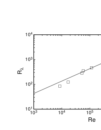
FIG. 1.: Taylor–scale Reynolds number $R_{\lambda}$ (for details on the determination see [11]) as a function of the nozzle-based Reynolds number $Re$. Dotted line: $R_{\lambda}=1.35\sqrt{Re}$.

The condition (2) for the Markov property was checked using the method proposed in ref. [11]. For all the data sets, the Markovian property was found to be valid for scales $r_{i}$ and differences of scales $\Delta r=r_{i+1}-r_{i}$ larger than the elementary step size $l_{mar}$, which turned out to be of the order of magnitude of the Taylor microscale $\lambda$ for all $Re$–numbers investigated.

Having determined the Markov length $l_{mar}$, the coefficients $D^{(1)}(u,r)$ and $D^{(2)}(u,r)$ can be estimated from the measured conditional moments $M^{(1)}$ and $M^{(2)}$ according to equation (7). The extrapolation towards $\Delta r=0$ was performed fitting linear functions to the measured $M^{(k)}$ in the intervall $l_{mar}\leq\Delta r\leq 2l_{mar}$ [16].

Figure 2 shows the resulting estimates for the coefficients $D^{(1)}$ and $D^{(2)}$ for the data set at $R_{\lambda}=1180$ as a function of the velocity increment at several scales $r$. The coefficients exhibit linear and quadratic dependencies on the velocity increment, respectively:

$$D^{(1)}(u,r) = -\gamma(r)u,$$ (9)

$$D^{(2)}(u,r) = \alpha(r)-\delta(r)u+\beta(r)u^{2}.$$ (10)

Equation (10) is found to describe the dependence of the $D^{(k)}$ on $u$ for all scales $r$ as well as for all Reynolds numbers investigated. By fitting the coefficients $D^{(k)}$ according to (10), it is thus possible to determine the scale dependence of the coefficients $\gamma$, $\alpha$, $\delta$ and $\beta$.

The constant and linear coefficient of $D^{(2)}$, $\alpha$ and $\delta$, turn out to be linear functions of the scale $r$ (see the inlet in fig. 3):

$$\alpha(r)=\alpha_{0}\frac{r}{\lambda},\qquad\delta(r)=\delta_{0}\frac{r}{\lambda}.$$ (11)

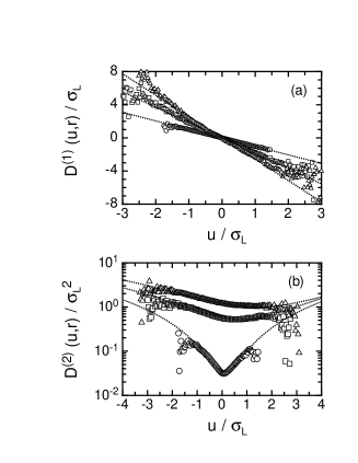
FIG. 2.: Coefficients $D^{(1)}(u,r)$ (a) and $D^{(2)}(u,r)$ (b) as functions of the velocity increment $u$ at $r=3\lambda$ (circles), $r=L/2$ (squares) and $r=L$ (triangles). The dotted curves correspond to linear (a) and polyonmial (b) (degree two) fits to the measured data.

As shown in figure 3, the slopes $\alpha_{0}$ and $\delta_{0}$ show strong dependencies on the Reynolds number and can be described by power laws in $Re$ with an scaling exponent of $-3/8$:

$$\alpha_{0}\approx 2.8Re^{-3/8},\qquad\delta_{0}\approx 0.68Re^{-3/8}.$$ (12)

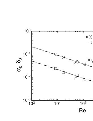
FIG. 3.: Coefficients $\alpha_{0}$ (circles) and $\delta_{0}$ (squares) defined in eqs. (10) and (11) as functions of the Reynolds number $Re$; dotted lines represent power laws in $Re$ with an scaling exponent of $-3/8$. The inlet displays $\alpha(r)$ as a function of the length scale $r$ for $R_{\lambda}=1180$.

A different result is obtained for the linear term $\gamma(r)$ of $D^{(1)}$, see figure 4. It turns out to be a universal function of $r/\lambda$ and is found to be well described by

$$\gamma(r)=\frac{2}{3}+c\sqrt{\frac{r}{\lambda}},$$ (13)

where $c=0.20\pm 0.01$.

FIG. 4.: The slope $\gamma(r)$ of $D^{(1)}$ (a) and the quadratic coefficient $\beta(r)$ of $D^{(2)}$ (b) as functions of the scale $r$ for several Reynolds numbers (see legend). $\gamma$ is close to a universal function of the scale $\rho=r/\lambda$ (the dotted line is a fit according to eq. (13)), the coefficient $\beta$ exhibits a strong dependence on the Reynolds number with a clear tendency towards the limiting value $\beta_{\infty}(r)$ given by equ. (17) (full line).

These results allow for a statement on the limiting case of infinite Reynolds numbers, $Re\rightarrow\infty$. According to eq. (12) the coefficients $\alpha$ and $\delta$ tend to zero [17]. $\gamma(r)$ does not depend on $Re$. Thus drift- and diffusion coefficient take the following simple form for $Re\rightarrow\infty$:

$$D^{(1)}_{\infty}(u,r) = -\gamma(r)u,$$ (14)

$$D^{(2)}_{\infty}(u,r) = \beta_{\infty}(r)u^{2}.$$ (15)

Based on this limiting result we discuss next implications for the structure functions $S_{u}^{n}(r)$. After the multiplication of the corresponding Fokker–Planck equation (6) for $p(u,r)$ with $u^{n}$ from left and successively integrating with respect to $u$, the equation

$$\frac{r\frac{\partial}{\partial r}S_{u}^{n}(r)}{nS_{u}^{n}(r)}=\gamma(r)-(n-1)\beta_{\infty}(r)$$ (16)

is obtained.

According to Kolmogorov’s four-fifth law, cf. [1], the third order structure function, $S_{u}^{3}(r)$, is proportional to $r$. Thus, for $n=3$, the left side of eq. (16) is equal to $1/3$ and $\beta_{\infty}(r)$ is given by:

$$\beta_{\infty}(r)=\frac{\gamma(r)}{2}-\frac{1}{6}.$$ (17)

For increasing Reynolds numbers, the experimental results for $\beta(r)$ in fact show a tendency towards the limiting value $\beta_{\infty}$ as given by eq. (17) (see fig. 4), but it is also clearly observed that the convergence is slow and that even the highest accessible Reynolds numbers are still far from this limiting case.

To summarize, the mathematical framework of Markov processes can succesfully be applied to characterize the stochastic behaviour of turbulence with increasing Reynolds number. Moreover, the description obtained by our method is complete in the sense that the entire information about the stochastic process, i.e. the information about any $N$–scale pdf $p(u_{1},r_{1};u_{2},r_{2};...;u_{N},r_{N})$, is encoded in the two coefficients $D^{(1)}(u,r)$ and $D^{(2)}(u,r)$, for which we find rather simple dependencies on their arguments $u$, $r$ and the Reynolds number.

The $Re$–dependence of the coefficients, especially of $D^{(2)}$, yields strong experimental evidence for a significant change of the stochastic process as the Reynolds number increases. This finding clearly contradicts the concept of a universal turbulent cascade and might also be of importance in large eddy simulations where the influence of the subgrid stress on the large scale dynamics of a turbulent flow is modeled under the assumption of universality.

It is easily verified that, according to eq. (16), the increase of $\beta(r)$ with $Re$ excludes the simple scaling laws proposed by Kolmogorov in 1941 [3] even for $Re\rightarrow\infty$. Furthermore, the universal functional dependence of $\gamma(r)$ on $r$ (eq. (13)) does not support the recently proposed constant value of $\gamma\approx 1/3$ [10, 18]. The obvious dependence of the coefficients $\gamma$ and $\beta$ on $r$ also contradicts the assumption that the structure functions exhibit scaling behaviour for all orders $n$, as can be derived from eq. (16).

With the limiting values for the coefficients $D^{(k)}$ as given by eq. (15), the stochastic process for infinite Reynolds numbers corresponds to an infinitely divisible multiplicativ cascade [19] as proposed in ref. [20]. However, from the slow convergence of the measured coefficient $\beta(r)$ towards its limiting value $\beta_{\infty}(r)$, it is obvious that turbulent data measured in typical laboratory experiments are still far from that special case. It therefore seems questionable to us whether models on turbulence established under the assumption of infinite Reynolds numbers can be tested in real-life experimental situations at all.

Acknowledgement: We gratefully acknowledge fruitful discussions with J.-F. Pinton, B. Castaing, F. Chilla and M. Siefert.

REFERENCES

- [1] K.R. Sreenivasan, R.A. Antonia, Ann. Rev. Fluid Mech., 29 435 (1997); U. Frisch, Turbulence, Cambridge 1996.
- [2] L.F. Richardson, Weather Prediction by Numerical Process, Cambridge University Press (1922);
- [3] A.N. Kolmogorov, Dokl. Akad. Nauk. SSSR 30, 301 (1941).
- [4] A.N. Kolmogorov, J. Fluid Mech. 12, 81 (1962); A.M. Oboukhov, J. Fluid Mech. 12, 77 (1962).
- [5] M. Lesieur, Turbulence in Fluids, Kluwer, Dordrecht, 1997.
- [6] Benzi, R. et al., Europhys. Lett. 24, 275 (1993).
- [7] A. Arneodo et al., Eurphys. Lett. 34, 411 (1996); R.A. Antonia, B.R. Pearson & T. Zhou, Phys. Fluids, 12(11), 3000 (2000).
- [8] Y. Malecot et al., Eur. Phys. J B 16 (3), 549–561 (2000); H. Kahalerras et al., Phys. Fluids 10 (4), 910–921 (1998).
- [9] V. L’vov & I. Procaccia, Phys. Rev. Lett. 76, 2898 (1996).
- [10] R. Friedrich & J. Peinke, Phys. Rev. Lett. 78, 863 (1997); R. Friedrich & J. Peinke, Physica D 102, 147 (1997).
- [11] Ch. Renner, J. Peinke & R. Friedrich, J. Fluid Mech 433, 383–409 (2001).
- [12] H. Risken, The Fokker-Planck equation, Springer-Verlag Berlin, 1984.
- [13] A.N. Komogorov, Math. Ann. 140, 415–458 (1931).
- [14] R. Friedrich, J. Zeller & J. Peinke, Europhys. Lett. 41, 143 (1998).
- [15] O. Chanal, B. Chabaud, B. Castaing and B. Hebral, Eur. Phys. J. B 17 (2), 309–317 (2000); O. Chanal, Ph.D. thesis, Institut National Polytechnique, Grenoble (1998).
- [16] Note that this method differs slightly from the one proposed in ref. [11], where first the were fitted as functions of the velocity increment . The coefficients of those fits were extrapolated towards in a second step.
- [17] Strictly speaking, only the coefficients nd tend to zero. But as the ratio scales like , the coefficients and at the integral length scale like: . On the other hand, the coefficient scales like the square root of . Thus: . The fact that grows faster than and justifies neglecting and in the limit .
- [18] V. Yakhot, Phys. Rev. E 57(2), 1737 (1998); J. Davoudi and M.R. Tabar, Phys. Rev. E 61, 6563 (2000).
- [19] P.-O. Amblard & J.-M. Brossier, Eur. Phys. J. B 12, 579 (1999).
- [20] B. Castaing, J. Phys. II France 6, 105 (1996).