Optimal use of time dependent probability density data to extract potential energy surfaces

Abstract

A novel algorithm was recently presented to utilize emerging time dependent probability density data to extract molecular potential energy surfaces. This paper builds on the previous work and seeks to enhance the capabilities of the extraction algorithm: An improved method of removing the generally ill-posed nature of the inverse problem is introduced via an extended Tikhonov regularization and methods for choosing the optimal regularization parameters are discussed. Several ways to incorporate multiple data sets are investigated, including the means to optimally combine data from many experiments exploring different portions of the potential. In addition, results are presented on the stability of the inversion procedure, including the optimal combination scheme, under the influence of data noise. The method is applied to the simulated inversion of a double well system to illustrate the various points.

I Introduction

To fully understand chemical dynamics phenomena it is necessary to know the underlying potential energy surfaces (PES) [1]. Surfaces can be obtained by two means: ab initio calculations [2, 3, 4, 5, 6] and the inversion of suitable laboratory data [7, 8, 9, 10, 11, 12, 13, 14]. This paper is concerned with an emerging class of laboratory data [15, 16, 17] with special features for inversion purposes. Traditional sources of laboratory data for inversion produce an indirect route to the potential requiring the solution of Schrödinger’s equation [18] in the process. An alternative suggestion [19, 20] has been put forth to utilize ultrafast probability density data from diffraction observations or other means [21, 22, 23, 24, 25, 26] to extract adiabatic potential surfaces. Such data consists of the absolute square of the wavefunction. Although the phase of the overall wavefunction is not available, there is sufficient information in this data to extract the potential fully quantum mechanically without the solution of Schrödinger’s equation. Instead, the proposed procedure rigorously reformulates the inversion algorithm as a linear integral equation utilizing Ehrenfest’s theorem [27] for the position operator. Additional attractive features of this algorithm are (a) the procedure may be operated non-iteratively, (b) no knowledge is required of the molecular excitation process leading to the data and (c) the regions where the potential may be reliably extracted are automatically revealed by the data.

Extensive efforts are under way to achieve the necessary temporal and spatial resolution of the probability density data necessary for inversion processes as well as for other applications [20]. In anticipation of these developments a number of algorithmic challenges require attention to provide the means to invert such data. This paper aims to build on the previous work [19] and address some of these needs. In particular this paper will consider (i) optimal choices for regularizing the inversion procedure, (ii) incorporation of multiple data sets and (iii) inclusion of data sampled at discrete time intervals. These concepts are developed and illustrated for the simulated inversion of a double well potential.

The paper is organized as follows. The basic inversion procedure and the model system are given in Section II. Based on the inversion algorithm derived in Ref. [19] an extended regularization procedure is presented in Section III followed by a discussion of a modified time integration scheme applicable to different types of experimental data sampling. This development naturally leads to consideration of an optimal combination of data from different measurements. A proof on how to optimally combine the data is given in Appendix A. The stability of this data combination procedure under the influence of noise is discussed as well. Section V summarizes the findings of this paper.

II The basic inversion procedure and the model system

The algorithms developed in this paper will be illustrated for a one-dimensional system but the generalization to higher dimensions is straightforward [28]: the major difference with higher dimensions is the additional computational effort involved. Atomic units are used throughout this work.

For a system whose dynamics is governed by the Schrödinger equation

$$\text{i}\frac{\partial}{\partial t}\psi(x,t)=\left[-\frac{1}{2m}\frac{\partial^{2}}{\partial x^{2}}+V(x)\right]\psi(x,t)$$ (1)

the time evolution of the average position obeys Ehrenfest’s theorem

$$0=m\frac{\text{d}^{2}}{\text{d}t^{2}}\int\!x\,\rho(x,t)\,\text{d}x+\int\!u(x)\,\rho(x,t)\,\text{d}x\;,$$ (2)

where $u(x)=\text{d}V(x)/{\text{d}x}$ and $\rho(x,t)=|\psi(x,t)|^{2}$. In this work the probability density $\rho(x,t)$ is assumed to be observed in the laboratory and the goal is to determine the potential energy surface (PES) $V(x)$ from the gradient $u(x)$.

Following [19], Eq.(2) can be used to construct a Gaussian least squares minimization problem to determine the PES gradient $u(x)$

$$J_{0}\{u(x)\}=\frac{1}{T}\int\limits_{0}^{T}\left[\int\!u(x)\,\rho(x,t)\,\text{d}x+m\frac{\text{d}^{2}}{\text{d}t^{2}}\int\!x\,\rho(x,t)\,\text{d}x\right]^{2}\text{d}t\;.$$ (3)

The time averaging acts as a filtering process to increase inversion reliability by gathering together more data. This will generally increase reliability which in principle is only limited by the exploratory ability of the wavepacket. Beyond some point in time little information on the potential may be gained by taking further temporal data starting from any potential initial condition.

Variation with respect to $u(x)$ results in a Fredholm integral equation of the first kind

$$\frac{\delta J_{0}\{u(x)\}}{\delta u(x)}=0\quad\Rightarrow\quad\int\!A(x^{\prime},x)\,u(x^{\prime})\,\text{d}x^{\prime}=b(x)$$ (4)

with righthand side (RHS)

$$b(x)=-\frac{m}{T}\int\limits_{0}^{T}\!\rho(x,t)\,\frac{\text{d}^{2}}{\text{d}t^{2}}\int\!x^{\prime}\,\rho(x^{\prime},t)\,\text{d}x^{\prime}\,\text{d}t$$ (5)

and symmetric, positive semidefinite kernel

$$A(x^{\prime},x)=\frac{1}{T}\int\limits_{0}^{T}\!\rho(x^{\prime},t)\rho(x,t)\,\text{d}t\;.$$ (6)

Treated as an inverse problem, Eq.(4) produces the desired PES gradient $u(x)$ as its solution. For numerical implementation we resort to the matrix version and its formal solution

$$\mathchoice{{\hbox{\boldmath$\displaystyle A$}}}{{\hbox{\boldmath$\textstyle A$}}}{{\hbox{\boldmath$\scriptstyle A$}}}{{\hbox{\boldmath$\scriptscriptstyle A$}}}\cdot\mathchoice{{\hbox{\boldmath$\displaystyle u$}}}{{\hbox{\boldmath$\textstyle u$}}}{{\hbox{\boldmath$\scriptstyle u$}}}{{\hbox{\boldmath$\scriptscriptstyle u$}}}\,\Delta x=\mathchoice{{\hbox{\boldmath$\displaystyle b$}}}{{\hbox{\boldmath$\textstyle b$}}}{{\hbox{\boldmath$\scriptstyle b$}}}{{\hbox{\boldmath$\scriptscriptstyle b$}}}\quad\Rightarrow\quad\mathchoice{{\hbox{\boldmath$\displaystyle u$}}}{{\hbox{\boldmath$\textstyle u$}}}{{\hbox{\boldmath$\scriptstyle u$}}}{{\hbox{\boldmath$\scriptscriptstyle u$}}}=\mathchoice{{\hbox{\boldmath$\displaystyle A$}}}{{\hbox{\boldmath$\textstyle A$}}}{{\hbox{\boldmath$\scriptstyle A$}}}{{\hbox{\boldmath$\scriptscriptstyle A$}}}^{-1}\cdot\mathchoice{{\hbox{\boldmath$\displaystyle b$}}}{{\hbox{\boldmath$\textstyle b$}}}{{\hbox{\boldmath$\scriptstyle b$}}}{{\hbox{\boldmath$\scriptscriptstyle b$}}}\,\Delta x^{-1};.$$ (7)

Here the integral in Eq.(4) is evaluated at points of equal spacing $\Delta x$.

This approach to seeking the PES has a number of attractive features [19]. The formulation requires no knowledge of any preparatory steps to produce a specific $\psi(x,0)$ which evolves freely to produce $\rho(x,t)$. The generation of $A(x,x^{\prime})$ and $b(x)$ depends only on $\rho(x,t)$ and begins when the observation process is started. Moreover, although this is a fully quantum mechanical treatment there is no need to solve Schrödinger’s equation to extract the PES. The dominant entries of $A(x,x^{\prime})$ and $b(x)$ automatically reveal the portions of the PES that may be reliably extracted. The linear nature of Eq.(4) is very attractive from a practical perspective.

Notwithstanding these attractions, a principal problem to manage is the generally singular nature of the kernel of the integral equation in Eq.(4). The kernel’s nullspace makes it difficult to solve the inverse problem and leads to an unstable and ambiguous solution $u(x)$, two characteristics that generally define the ill-posedness of inverse problems. There are two major reasons for the ill-posedness of the inverse problem in Eqs. (4) and (7). Firstly, it is not possible to continuously monitor the wavepacket with arbitrary accuracy and information is lost due to discrete data sampling in space and time. Secondly, the ill-posedness is due to the wavepacket only exploring a subspace of the PES. In regions untouched by the wavepacket with $\rho(x,t)\!\approx\!0$ for all observation times $t$ the kernel entries vanish as $A(x,x^{\prime})\!=\!A(x^{\prime},x)\!=\!\frac{1}{T}\int_{0}^{T}\rho(x,t)\rho(x^{\prime},t)\,\text{d}t\!\approx\!0$. Hence these regions correspond to zero-entry rows and columns in the kernel matrix $\textstyle A$ and constitute its nontrivial nullspace. In general, the solution $u(x)$ will only be reliable in regions where $\rho(x,t)$ has significant magnitude during its evolution. The inversion procedure can manage the null space with the help of a suitable regularization procedure. Singular value decomposition and iterative solution schemes are available (cf. [29, 30] for an overview), but here we will employ extended Tikhonov regularization (see Section III).

The procedures developed in this paper are applied to a simulated inversion with a system taken to have a slightly asymmetric double well potential [31]

$$V(x)=\frac{\Delta}{2q_{0}}(x-q_{0})+\frac{\hat{V}-\Delta/2}{q_{0}^{4}}(x-q_{0})^{2}(x+q_{0})^{2}+\Delta$$ (8)

with parameters

$$q_{0} = 1.0$$ (9)

$$\Delta = 0.000\,257\quad\text{(asymmetry)}$$ (10)

$$\hat{V} = 0.006\,25\phantom{7}\quad\text{(barrier height)}\;.$$ (11)

In the work of N. Došlić et al. [31] this PES represents a one dimensional model for the intramolecular proton transfer in substituted malonaldehyde (see Fig. 1). The particle mass is accordingly that of hydrogen.

The wavepacket propagations to obtain the simulated $\rho(x,t)$ data employed the split operator method (cf. [32, 33]). For propagation as well as inversion we used a grid with 8192 points over the range $-4.0\leqslant x\leqslant 4.0$. A time step $\Delta t_{\text{prop}}=3$ was chosen and total propagation time was $T=1200$. The small values of $\Delta t_{\text{prop}}$ and $\Delta x_{\text{prop}}$ ensured good convergence of the numerical propagation procedure.

The initial wavefunctions were normalized Gaussian wavepackets of width $\sigma=0.05$. As stated earlier, the inversion algorithm requires no knowledge of how these packets were formed, but generally one may assume that a suitable external laser field was applied for times $t<0$. The initial packets were placed at the left (L) and right minimum (R) of the PES, on top of the barrier (T), and at a location high on the potential (H). The wavepacket positions are illustrated in Fig. 1 and their exact values, the associated average energies and the classical turning points at these energies are given table I. The inversion process employed a time step and grid spacing that differed from those used in the propagation, as high spatial and temporal resolution is difficult to attain in the laboratory. Hence, we employed only a portion of all the available propagation data $\rho(x,t)$ in time and space. We will present inversion results using every 16th propagation grid point (i.e., $\Delta x=16\cdot\Delta x_{\text{prop}}$) and every fifth available snapshot (i.e., $\Delta t=5\cdot\Delta t_{\text{prop}}$); even fewer snapshots could be used over a longer period of time with the criterion that roughly the same total amount of data is retained. The inversion results from these lower resolution data are very encouraging.

The kernel matrices $\textstyle A$ for condition H and T are shown in Fig. 2; similar plots apply to the cases L and R. The kernels are symmetric with respect to $x\!=\!x^{\prime}$ and their values cover a large dynamic range from $\thicksim 10^{3}$ down to $10^{-8}$ on the plotted domain. Significant entries are found predominantly on the matrix diagonal, close to the origin of the wavepacket, and also in the vicinity of the classical turning points. Beyond the classical turning points at a distance of approximately $\pm 2.0$ the kernel values fall off very rapidly for both configurations.

For configuration H in Fig. 2a the initial narrow gaussian is peaked at the hydrogen distance $x_{0}\!=\!1.75$ with corresponding large entries around $(x,x^{\prime})\!\approx\!(2,2)$. The wavepacket starts to spread and acquires momentum as it slides down the PES, which results in the broadening diagonal trace observed as the central structure in Fig. 2a. When the wavepacket reaches its lefthand turning point it spreads further (star structure around $(x,x^{\prime})\!\approx\!(-1.75,-1.75)$) before it returns. This pattern coincides with the motion of the average position $\langle x(t)\rangle$ displayed for configuration H in Fig. 4a.

Even higher symmetry can be observed for configuration T’s kernel matrix $\textstyle A$ in Fig. 2b. The initial gaussian remains centered around $x_{0}\!=\!0.0052$ and spreads to the left and righthand well only. This is further supported by the motionless average position $\langle x(t)\rangle$ in Fig. 4a. Hence large entries in $\textstyle A$ result in the vicinity of $(x,x^{\prime})\!=\!(x_{0},x_{0})$ and the wavepacket’s symmetrical spread to the left and righthand side of the PES produces the spikes along the $x$-axis for $x^{\prime}\!=\!0$. Due the kernel’s symmetry these spikes reappear as lines along the $x^{\prime}$-axis for $x\!=\!0$. Large contributions for $x\!=\!x^{\prime}$ will again lead to a pronouced diagonal and add to the snowflake appearance of Fig. 2b.

The features of the kernels in Fig. 2 coincide with the nature of the inverse problem mentioned earlier: symmetry, ill-posedness, and automatic identification of the range where the PES may be be reliably extractable (i.e., where the kernel entries are large). For configuration H the relevant range is $-2\lesssim x\lesssim 2$ and for configuration T only the vicinity of the barrier top should yield reliable PES information. In both cases we cannot expect reasonable solutions beyond $\pm 2.0$, which coincides with the classical turning points given in table I.

III An improved regularization procedure

Tikhonov regularization [34] is straightforward to implement with simple control provided by suitable weight parameters. It provides a well defined means to stabilize the inversion and extract reliable PES information in those regions allowed by the data.

This investigation goes beyond the initial work [19] to carefully explore various regularization options. Regularization has the goal of improving the accuracy of the solution, assuring stability and ease of use including computational simplicity. The functional $J_{0}$ was augmented by a regularization term involving a set of increasingly higher order differential operators acting on $u(x)$

$$J_{1}\{u(x)\}=J_{0}\{u(x)\}+\sum_{\nu=0}^{N}\alpha_{\nu}\xi^{-1}\int\left[\left(\xi\frac{\text{d}}{\text{d}x}\right)^{\nu}u(x)\right]^{2}\,\text{d}x\;,$$ (12)

with real coefficients $\alpha_{\nu}>0$ and a reference length $\xi$. In practice $\xi$ may be thought of as the spatial resolution of the data and in the present numerical simulation it was taken as $\Delta x$. For a multidimensional system, $\xi$ and $\alpha_{\nu}$ will become direction dependent tensors. The parameter $\xi$ acts to ensure that all the new terms added to $J_{0}$ have the same units as $[u]^{2}$ as well as permits comparison of the roles of the dimensionless regularization parameters $\alpha_{\nu}$ for different $\nu$ and different grid spacings $\Delta x$.

The previous work [19] did not employ a reference length as only the $\nu=0$ regularization term was considered. The parameter $\alpha_{0}$ penalizes the value of $u(x)$. The new terms go beyond and impose extra pressure on the gradient ($\nu=1$), the curvature ($\nu=2$) of $u(x)$, etc. .

Variation of $J_{1}$ with respect to $u(x)$ yields the modified inversion prescription

$$\int\!\left[A(x^{\prime},x)+\delta(x-x^{\prime})\cdot\sum_{\nu=0}^{N}\alpha_{\nu}\xi^{-1}\left(-\xi^{2}\frac{\text{d}^{2}}{\text{d}x^{\prime 2}}\right)^{\nu}\right]\,u(x^{\prime})\,\text{d}x^{\prime}=b(x)\;.$$ (13)

The sum added to $J_{0}$ in Eq.(12) for regularization consisted of purely positive terms with derivatives of up to $N$th order, resulting in an alternating series of only even derivatives up to order $2N$ in Eq.(13). Moreover, the Fredholm integral equation of the first kind has been transformed into an integro-differential equation for $u(x)$ with the added terms dominating in the regions where kernel is singular.

Due to the rapid growth in the order of the derivatives it is often sufficient to set $N=2$, i.e., retaining standard, gradient, and curvature Tikhonov regularization. For numerical application Eq.(13) may be transformed into the matrix problem

$$\left[\mathchoice{{\hbox{\boldmath$\displaystyle A$}}}{{\hbox{\boldmath$\textstyle A$}}}{{\hbox{\boldmath$\scriptstyle A$}}}{{\hbox{\boldmath$\scriptscriptstyle A$}}}+\alpha_{0}\Delta x^{-2}\,\openone-\alpha_{1}\,\mathchoice{{\hbox{\boldmath$\displaystyle D$}}}{{\hbox{\boldmath$\textstyle D$}}}{{\hbox{\boldmath$\scriptstyle D$}}}{{\hbox{\boldmath$\scriptscriptstyle D$}}}+\alpha_{2}(\Delta x)^{2}\,\mathchoice{{\hbox{\boldmath$\displaystyle Q$}}}{{\hbox{\boldmath$\textstyle Q$}}}{{\hbox{\boldmath$\scriptstyle Q$}}}{{\hbox{\boldmath$\scriptscriptstyle Q$}}}\right]\cdot\mathchoice{{\hbox{\boldmath$\displaystyle u$}}}{{\hbox{\boldmath$\textstyle u$}}}{{\hbox{\boldmath$\scriptstyle u$}}}{{\hbox{\boldmath$\scriptscriptstyle u$}}}\,\Delta x=\mathchoice{{\hbox{\boldmath$\displaystyle b$}}}{{\hbox{\boldmath$\textstyle b$}}}{{\hbox{\boldmath$\scriptstyle b$}}}{{\hbox{\boldmath$\scriptscriptstyle b$}}}\,,$$ (14)

employing the unit matrix $\openone$, as well as the second

$$\mathchoice{{\hbox{\boldmath$\displaystyle D$}}}{{\hbox{\boldmath$\textstyle D$}}}{{\hbox{\boldmath$\scriptstyle D$}}}{{\hbox{\boldmath$\scriptscriptstyle D$}}}=\frac{1}{(\Delta x)^{2}}\left(\begin{array}[]{rrrrr}-2&1&&&0\\ 1&-2&1&&\\ &\ddots&\ddots&\ddots&\\ &&1&-2&1\\ 0&&&1&-2\end{array}\right)\;,$$ (15)

and the forth order differentiation band matrices

$$\mathchoice{{\hbox{\boldmath$\displaystyle Q$}}}{{\hbox{\boldmath$\textstyle Q$}}}{{\hbox{\boldmath$\scriptstyle Q$}}}{{\hbox{\boldmath$\scriptscriptstyle Q$}}}=\frac{1}{(\Delta x)^{4}}\left(\begin{array}[]{rrrrrrrrr}6&-4&1&0&&&&\cdots&0\\ -4&6&-4&1&0&&&&\vdots\\ 1&-4&6&-4&1&0\\ 0&1&-4&6&-4&1&0\\ \vdots&\ddots&\ddots&\ddots&\ddots&\ddots&\ddots&\ddots\end{array}\right)\;.$$ (16)

These are simple differencing expressions for the derivatives involved. Higher order expressions for the derivatives could be considered, but finite data resolution and laboratory noise will generally not warrant or support the added complexity.

To investigate the inverse solution’s dependence on the various regularization parameters in Eq.(14) several parameter scans for all four configurations L, T, R, H were performed for different resolutions $\Delta x$ and combinations of $\alpha_{\nu}$-parameters. For the discussion in this paper, we selected typical results for the situation of H with $\Delta x=16\Delta x_{\text{prop}}$. The curves in Fig. 3 show the solution defect $|\Delta u|$ and the system defect $|\Delta s|$ as defined below in Eqs.(17) and (20). While only $|\Delta s|$ is an experimentally accessible figure of merit, an investigation of $|\Delta u|$ here allows for quantifying the quality of the inverse solution. For both error measures reported the plots are generated for each $\alpha_{\nu}$ independently while the others are kept zero.

Figures 3a and 3b display the solution defect

$$|\Delta u|=\left[\frac{1}{x_{b}-x_{a}}\int\limits_{x_{a}}^{x_{b}}\left(\,u_{\text{exact}}(x)-u(x)\,\right)^{2}\,\text{d}x\right]^{1/2}\;.$$ (17)

Figure 3a is computed with $x_{a}=-2.0$, $x_{b}=2.0$ (i.e. the central domain indicated in Fig. 2 and table I within which the inversion is expected to be valid) and Fig. 3b with $x_{a}=-4.0$, $x_{b}=4.0$ (i.e., the full simulation range). The differences between the two cases are striking. The corresponding solution defects show a completely different shape with minima that differ by several orders of magnitude in $\alpha_{\nu}$. In Fig. 3b the magnitude of the error in the active domain $-2\lesssim x\lesssim 2$ is overestimated. This behavior in Fig. 3b is due to large deviations between the exact gradient and the inversion solution for the gradient, which cannot be recovered reliably in the domain’s outer limits. Thus we conclude that $|\Delta u|$ scans should only be computed over the regions actually reached to a significant degree by the wavepacket (cf., Fig. 3a) to achieve reliable estimates of the inversion quality.

The latter point is illustrated in Figs. 4b and 4c with the inverted results for $u(x)$ ane $V(x)$ with pure $\alpha_{1}$ regularization of configurations H/H₁ where $\alpha_{1}$ is given in table II. The two cases H/H₁ differ in the domain employed in the inversion (i.e., the active domain for H and the full domain for H₁) and in the choice of optimal $\alpha_{1}$ determined according to the $|\Delta u|$ scans. Thus we further conclude that the inversion process should be confined to the active domain to maintain stability.

To find suitable integration regions from the laboratory data the normalized lefthand

$$\sigma^{2}_{\ell}(t)={\int\limits_{-\infty}^{\langle x\rangle}(x-\langle x\rangle)^{2}\rho(x,t)\,\text{d}x}\left/\int\limits_{-\infty}^{\langle x\rangle}2\rho(x,t)\,\text{d}x\right.$$ (18)

and righthand variance

$$\sigma_{\text{r}}^{2}(t)={\int\limits_{\langle x\rangle}^{\infty}(x-\langle x\rangle)^{2}\rho(x,t)\,\text{d}x}\left/\int\limits_{\langle x\rangle}^{\infty}2\rho(x,t)\,\text{d}x\right.$$ (19)

of the position operator can be helpful. Together with the position average $\langle x\rangle$ they can provide an estimate for the PES domain predominantly covered by the wavepacket motion. We present all three quantities ($\langle x(t)\rangle$ and $\sigma_{\ell}(t),\sigma_{\text{r}}(t)$ as grey shaded regions) in Fig. 4a. The results clearly show that for configuration H the range $-2\lesssim x\lesssim 2$ is suitable. For configurations L, T, R an even smaller range is best (cf., table II).

All the computations revealed that a gradient Tikhonov regularization based on $\alpha_{1}$ performs better than the standard regularization based on $\alpha_{0}$ utilized earlier [19]. There is some additional improvement in choosing the curvature regularization $\alpha_{2}$, but we found it to be less stable for coarse grids, which will be the standard situation in actual application.

We also found little improvement in mixing the different regularization schemes. In general the $\alpha_{\nu}$ regularization with the largest errors masks the positive effects of the others. Hence for all cases of the PES reconstruction we utilized only $\alpha_{1}$ regularization (cf., the inversion in Figs. 4a and 4b with the optimal parameters given in table II).

As a measure of inversion quality and the role of regularization, we desire a quantity that is strictly available from the laboratory data $\rho(x,t)$. A good choice is the system defect $|\Delta s|$ defined by the norm of satisfying the system equation (4) with the inverse solution $u(x)$ found via Eq. (13)

$$|\Delta s|=\left[\frac{1}{L}\int\left(\,b(x)-\int A(x,x^{\prime})u(x^{\prime})\,\text{d}x^{\prime}\,\right)^{2}\,\text{d}x\right]^{1/2}\;.$$ (20)

The values of $|\Delta s|$ will depend on the regularization parameters $\alpha_{\nu}$. Weak regularization will produce a small value of $|\Delta s|$, but likely artificial structures in the PES. Over regularization will result in a smooth PES, that is systematically in error with diminished influence from the kernel $A(x,x^{\prime})$ on the inverse solution. The best choice for the $\alpha_{\nu}$ is generally where $|\Delta s|$ has risen and leveled off in a stable region as shown in Fig. 3c. The figure shows that $|\Delta s|$ naturally tends to zero as $\alpha_{\nu}\to 0+$ and monotonically rises until it reaches a plateau. There is very good agreement between the values of $\alpha_{\nu}$ which show good results for $|\Delta u|$ in Fig. 3a and the stable regularization region identified in Fig. 3c. Thus $|\Delta s|$ should be of practical utility in assigning regularization parameter values.

The generally self-similar structures in Figs. 3a and 3c suggest that every regularization operator has a roughly similar effect. This added robustness is also attractive for practical application if it holds up regardless of the system.

IV Combining distinct sets of laboratory data

Sections IV A and IV B will cover different approaches to combining distinct sets of laboratory density data. Finally Section IV C will explore the impact of data noise on the inversion.

A Optimal combination of experimental data

The functional $J_{0}\{u(x)\}$ in its original form in Eq.(3) is expressed in terms of a uniform, continuous time integration of observed $\rho(x,t)$ data. However, experimental circumstances including measurements at discrete snapshots in time or changes in the quality of data sampling may necessitate employing a weight function $\omega(t)$ for a generalized approach to the time integration in the functional $J_{0}$. Thus we define $\hat{J}_{0}$ as

$$\hat{J}_{0}\{u(x)\}=\int\limits_{0}^{\infty}\left[\int\!u(x)\,\rho(x,t)\,\text{d}x+m\frac{\text{d}^{2}}{\text{d}t^{2}}\int\!x\,\rho(x,t)\,\text{d}x\right]^{2}\omega(t)\,\text{d}t\;.$$ (21)

The choice $\omega(t)=[\,\Theta(t)-\Theta(t-T)\,]/T$, with $\Theta$ being the Heaviside step function, will reduce $\hat{J}_{0}$ to $J_{0}$.

Variation of Eq.(21) leads to a modified inverse problem

$$\frac{\delta\hat{J}_{0}\{u(x)\}}{\delta u(x)}=0\quad\Rightarrow\quad\int\!\hat{A}(x^{\prime},x)\,u(x^{\prime})\,\text{d}x^{\prime}=\hat{b}(x)\;,$$ (22)

with the new kernel

$$\hat{A}(x^{\prime},x)=\int\limits_{0}^{\infty}\!\rho(x^{\prime},t)\rho(x,t)\,\omega(t)\,\text{d}t$$ (23)

and RHS

$$\hat{b}(x)=-m\int\limits_{0}^{T}\!\omega(t)\,\rho(x,t)\,\frac{\text{d}^{2}}{\text{d}t^{2}}\int\!x^{\prime}\,\rho(x^{\prime},t)\,\text{d}x^{\prime}\,\text{d}t\;.$$ (24)

The weight $\omega(t)$ does not alter the regularization terms in Eq.(13). If $\hat{b}(x)$ is rewritten using partial integration over time, then the weight function must be considered in this process.

The above equations were applied to two generic cases. First, we considered data gathered as snapshots in time i.e., $\omega(t)=\sum_{j=1}^{T}\,\delta(t_{j}-t)$, and evaluated Eqs. (23) and (24) with this weight. This procedure simply reduced all time integrations to sums over the sampled $\rho$ data. Next, we considered the case in which the measurement process has been divided into two continuous time intervals of length $T_{1}$ and $T_{2}$ separated by a period of time $\tau$. A reasonable choice of weights would either be

$$\omega(t)=\frac{\Theta(t)-\Theta(t-T_{1})}{T_{1}+T_{2}}+\frac{\Theta(t-\tau-T_{1})-\Theta(t-\tau-T_{1}-T_{2})}{T_{1}+T_{2}}\;.$$ (25)

or

$$\omega(t)=\frac{\Theta(t)-\Theta(t-T_{1})}{T_{1}}+\frac{\Theta(t-\tau-T_{1})-\Theta(t-\tau-T_{1}-T_{2})}{T_{2}}\;.$$ (26)

The choice depends on the desired emphasis to be given to the two data intervals. Here we chose to give the longer interval a larger contribution in $\hat{A}(x,x^{\prime})$ than the shorter one, and this can be better achieved with using Eq.(25); this choice is reasonable, provided the measured data $\rho(x,t)$ in both intervals are of comparable quality. Clearly many other issues can be incorporated into the choice of $\omega(t)$ dictated by what is known about the nature of the data and the information sought about the PES.

The kernel is now

$$\hat{A}(x^{\prime},x)=\frac{1}{T_{1}+T_{2}}\left(\int\limits_{0}^{T_{1}}+\int\limits_{T_{1}+\tau}^{T_{1}+\tau+T_{2}}\right)\rho(x^{\prime},t)\rho(x,t)\,\text{d}t$$ (27)

and the RHS reads

$$\hat{b}(x)=-\frac{m}{T_{1}+T_{2}}\left(\int\limits_{0}^{T_{1}}+\int\limits_{T_{1}+\tau}^{T_{1}+\tau+T_{2}}\right)\rho(x,t)\,\frac{\text{d}^{2}}{\text{d}t^{2}}\int\!x^{\prime}\,\rho(x^{\prime},t)\,\text{d}x^{\prime}\,\text{d}t\;.$$ (28)

The interpretation of the weight in Eq.(25) is associated with performance of the inversion with an interrupted gathering of data from a single experiment. To explore this point further it is useful to rewrite Eqs.(27) and (28) as

$$\int\left[\,A_{1}(x,x^{\prime})+A_{2}(x,x^{\prime})\,\right]u(x^{\prime})\,\text{d}x^{\prime}=b_{1}(x)+b_{2}(x)\;,$$ (29)

where the indices “1” and “2” denote the evident two data time domains. In this form the gathering of data from one interrupted experiment can also be interpreted as finding the simultaneous solution to the inverse problem of two different experiments. These two experiments could possibly be prepared with distinct controls could, for example, explore different regions of the PES.

We found that it is optimal to simply combine these sets of data by addition as indicated in Eq.(29). This procedure will yield an inverse solution $u_{0}(x)$ with accuracy greater than a linear combination $u(x)=\mu u_{1}(x)+\nu u_{2}(x)$ of separate solutions to the individual problems “1” and “2” as explained below.

Consider two experiments that yield two different inverse solutions satisfying their respective system equation

$$\int A_{1,2}(x,x^{\prime})u_{1,2}(x^{\prime})\,\text{d}x^{\prime}=b_{1,2}(x)\;.$$ (30)

Naturally there should be only a unique exact $u_{\text{ex.}}(x)$ for the physical system. Hence both system solutions $u_{1,2}$ in Eq.(30) can be decomposed into the exact solution and contamination pieces from the kernel’s nullspace

$$u_{1,2}(x)=u_{\text{ex.}}(x)+a_{1,2}(x)+r_{1,2}(x)\;.$$ (31)

The functions $a_{1,2}$ and $r_{1,2}$ are associated with the nullspace of the two kernels with $a_{1,2}(x)\in\ker(A_{1})\cap\ker(A_{2})$ being the contamination from the common nullspace of $A_{1}$ and $A_{2}$ and $r_{1,2}(x)$ the residual contribution unique to the respective kernel. The goal is to use the data to find an optimal solution $u_{0}(x)$ with the smallest possible nullspace contribution.

Exploiting the linearity of the inverse problem, we may add the two pieces of Eq.(30) to get

$$\int A_{1}(x,x^{\prime})u_{1}(x^{\prime})\,\text{d}x^{\prime}+\int A_{2}(x,x^{\prime})u_{2}(x^{\prime})\,\text{d}x^{\prime}=b_{1}(x)+b_{2}(x)\;.$$ (32)

This doesn’t fully satisfy Eq.(29) and it is in general not possible to construct the optimal solution $u_{0}(x)$ as a linear combination $u_{0}(x)=\mu\,u_{1}(x)+\nu\,u_{2}(x)$ with constant coefficients $\mu,\nu$. To elucidate this point, we insert $u_{0}(x)$ into Eq.(29) and with the help of Eqs.(30) and (31) we get the cross terms

$$\int A_{1}(x,x^{\prime})u_{2}(x^{\prime})\,\text{d}x^{\prime} = b_{1}(x)+\int A_{1}(x,x^{\prime})r_{2}(x^{\prime})\,\text{d}x^{\prime}=b_{1}(x)+{}_{1}\varepsilon_{2}(x)$$ (33)

$$\int A_{2}(x,x^{\prime})u_{1}(x^{\prime})\,\text{d}x^{\prime} = b_{2}(x)+\int A_{2}(x,x^{\prime})r_{1}(x^{\prime})\,\text{d}x^{\prime}=b_{2}(x)+{}_{2}\varepsilon_{1}(x)\;,$$ (34)

where the prefactors $\mu$, $\nu$ have been omitted. Hence $u_{0}(x)$ is not an optimal solution of Eq.(29) since it leaves errors ${}_{i}\varepsilon_{j}(x)$ that cannot be eliminated. However, by employing Eq. (29) and adding the kernels and RHSs we can improve the quality of the inversion. No error terms like ${}_{i}\varepsilon_{j}(x)$ will appear since by construction the resulting $u_{0}(x)$ can be decomposed as $u_{0}(x)=u(x)+a_{0}(x)$. A contribution from $r_{0}(x)$ as in Eq.(31) will not arise, as proved in Appendix A. Thus, the solution of the combined problem will gain in quality by virtue of the reduced nullspace of the new kernel $A_{1}+A_{2}$.

These optimality results are rigorous but it must be added that in general any combination of a finite amount of data will not fully eliminate the nullspace. However in the cases under comparison here the assumption that a similar degree of robustness can be attained certainly holds true.

As argued above, we chose the weighting function in Eq.(25) to result in observation-duration proportional entries in $A_{1}(x,x^{\prime})$ and $A_{2}(x,x^{\prime})$. Hence it is quite natural to add $A=A_{1}+A_{2}$. However, choosing the approach Eq.(26) normalizes each data set independently. This logic naturally leads to considering the optimal combination of data to form $A=\sigma A_{1}+\delta A_{2}$ where $\sigma$ and $\delta$ are positive constants. This specially weighted form, or a positive definite combination $A=(1-\beta)A_{1}+\beta A_{2}$ with $\beta\in(0,1)$, might be useful especially in the presence of different degrees of noise in the two data sets. An iterative numerical scheme to optimize $\beta$ could then help to improve the solution by minimizing the effects of nullspace contamination.

The optimal combination of data by addition of kernels $A_{i}(x,x^{\prime})$ and RHSs $b_{i}(x)$ presented above was applied to the double well system with results for the gradient $u(x)$ and PES $V(x)$ shown in Fig. 5. Information was successively added to the kernel $A(x,x^{\prime})$ by combining the data sets to form LT, LTR, and LTRH with the notation based on the initial conditions shown in Fig. 1. In each case all configurations are weighted equally. The optimal $\alpha_{1}$ values employed and defect measures are given in table II.

While the individual inverse problem solutions based on L, T, R, and H reproduce the potential in their respective neighborhoods quite well, they fail to give adequate results for the other portions of the potential. On the other hand, the reconstruction of large parts of the PES is successful if we optimally combine the data of the three experiments LTR. However, contrary to intuition, we observe that the solution is less satisfactory from combining all the data LTRH; some additional oscillations appear along with a dip in the vicinity of the initial wavepacket for H. Apparently the nullspace of the expanded domain cannot be fully managed by $\alpha_{1}$ regularization alone; no attempt was made to simultaneously introduce $\alpha_{0}$ and $\alpha_{2}$ regularization.

B Other combinations of data

Several other schemes for combining the raw density data can be envisioned, apart from the approach in Section IV A. One candidate would be the direct combination of $\rho(x,t)$ data from different experiments. As an illustration we will treat the case of two different $\rho$’s with

$$\rho(x,t)=\rho_{1}(x,t)+\varepsilon\rho_{2}(x,t)$$ (35)

and $\varepsilon$ being a positive constant. This combination is physically acceptable, as Ehrenfest’s theorem in Eq.(2) is linear in the probability density. Insertion of this sum into the functional $J_{0}\{u(x)\}$ and variation with respect to $u(x)$ will yield a formulation analogous to the one describing inversion under the influence of noise in the data (see Section IV C) in Eq.(39) upon comparison of Eqs.(37) and (35).

The terms proportional to $\varepsilon^{0}$ and $\varepsilon^{2}$ will exactly correspond to what was found earlier in Eq.(29). However, the terms proportional to $\varepsilon$ represent a cross correlation between $\rho_{1}$ and $\rho_{2}$. These cross terms can be significant, and they act to introduce an element of undesirable structure, often oscillatory, in the equations determining $u(x)$. On physical grounds it is also artificial to directly correlate the independent experimental data $\rho_{1}$ and $\rho_{2}$ when seeking $u(x)$.

Hence, the scheme of adding together the bare $\rho$-data is expected to produce unreliable results. To support this argument we present a test on such a $\rho$-combination consisting of the sum of all four densities of the initial configurations L, T, R, and H

$$\rho_{\Sigma}(x,t)=\rho_{L}(x,t)+\rho_{T}(x,t)+\rho_{R}(x,t)+\rho_{H}(x,t)\;.$$ (36)

The corresponding inverted gradient and PES respectively are shown in Figs. 5a and 5b. The solution is rather poor and far worse than the LTRH combination using the same data. This result should not be taken to construe that other combinations of data might not give satisfactory results. However, the combination of $A_{i}$ and $b_{i}$ in Section IV A is quite natural and produces excellent inversion results.

C The influence of noise on the inversion

Any real $\rho$-data will always be contaminated by some degree of noise. In an additive model this noise contaminated data $\rho_{\text{n}}(x,t)$ can be represented as

$$\rho_{\text{n}}(x,t)=\rho(x,t)+\varepsilon\gamma(x,t)\;,$$ (37)

where $\varepsilon>0$ is a ordering parameter and the noise is described by the spatio-temporal function $\gamma(x,t)$. We assume that $\gamma(x,t)$ is a randomly varying function with vanishing average contribution and free from systematic error such that

$$\frac{1}{T}\int\limits_{0}^{T}\gamma(x,t)\sigma(x,t)\,\text{d}t\quad\stackrel{{\scriptstyle T\to\infty}}{{\longrightarrow}}\quad 0$$ (38)

for any function $\sigma(x,t)$ of bounded norm over time that is not correlated with $\gamma(x,t)$.

Inserting the ansatz in Eq.(37) into the functional $J_{0}\{u(x)\}$ in Eq.(3) and taking the first variation, the equation determining $u(x)$ is obtained

$$\frac{1}{T}\int\!\int\limits_{0}^{T}\rho(x^{\prime},t)\rho(x,t)\,\text{d}t\,u(x^{\prime})\;\text{d}x^{\prime}+\frac{\varepsilon}{T}\int\!\int\limits_{0}^{T}\rho(x^{\prime},t)\gamma(x,t)\,\text{d}t\;u(x^{\prime})\,\text{d}x^{\prime}$$ (39)

$$+\frac{\varepsilon}{T}\int\!\int\limits_{0}^{T}\gamma(x^{\prime},t)\rho(x,t)\,\text{d}t\,u(x^{\prime})\;\text{d}x^{\prime}+\frac{\varepsilon^{2}}{T}\int\!\int\limits_{0}^{T}\gamma(x^{\prime},t)\gamma(x,t)\,\text{d}t\;u(x^{\prime})\,\text{d}x^{\prime}$$ (40)

$$= -\frac{m}{T}\int\limits_{0}^{T}\rho(x,t)\,\frac{\text{d}^{2}}{\text{d}t^{2}}\int x^{\prime}\rho(x^{\prime},t)\,\text{d}x^{\prime}\;\text{d}t-\varepsilon\frac{m}{T}\int\limits_{0}^{T}\rho(x,t)\,\frac{\text{d}^{2}}{\text{d}t^{2}}\int x^{\prime}\gamma(x^{\prime},t)\,\text{d}x^{\prime}\;\text{d}t$$ (42)

$$-\varepsilon\frac{m}{T}\int\limits_{0}^{T}\gamma(x,t)\,\frac{\text{d}^{2}}{\text{d}t^{2}}\int x^{\prime}\rho(x^{\prime},t)\,\text{d}x^{\prime}\;\text{d}t-\varepsilon^{2}\frac{m}{T}\int\limits_{0}^{T}\gamma(x,t)\,\frac{\text{d}^{2}}{\text{d}t^{2}}\int x^{\prime}\gamma(x^{\prime},t)\,\text{d}x^{\prime}\;\text{d}t\;.$$

The terms proportional to $\varepsilon^{0}$ recover the original unperturbed system in Eqs.(4-6). Assuming the data noise level to be small, the terms in $\varepsilon^{2}$ on both sides of Eq.(39) can be neglected.

We first turn to the kernel side of Eq.(39) and denote all terms in $\varepsilon^{1}$ as the error kernel $\delta A(x,x^{\prime})$

$$\delta A(x,x^{\prime})=\frac{\varepsilon}{T}\int\limits_{0}^{T}\gamma(x^{\prime},t)\rho(x,t)\,\text{d}t+\frac{\varepsilon}{T}\int\limits_{0}^{T}\rho(x^{\prime},t)\gamma(x,t)\,\text{d}t\;.$$ (43)

Each term involves the computation of two-point spatial correlations between functions. However, the functions $\gamma$ and $\rho$ are uncorrelated, and the temporal integral of their product is expected to result in only small random contributions to the kernel over $x$ and $x^{\prime}$, especially for longer time integration as follows from Eq. (38). Following similar logic, the terms proportional to $\varepsilon^{1}$ on the RHS of Eq.(39) should be negligible, especially for long time integration. Neglecting the $\varepsilon^{2}$ terms finally leaves only the first term proportional to $\varepsilon^{0}$ on the RHS.

Hence, the functional $J_{0}$ exhibits some inherent capability to deal with slightly noisy data. The time integration process averages out these noise effects so that they should have a decreasing impact on the inverse solution $u(x)$. Longer periods of temporal data should make their behavior better.

These results are also in accordance with the stability analysis presented in [19]. Resorting to the matrix version of the inverse problem (cf., Eq.(14)) the authors proved (Eq.(25) in Ref. [19]) that the relative error in the solution ${u}$ after regularization is bounded by the relative errors in the data $\delta{b}$ and $\delta{A}$.

Moreover it was found (Eqs.(41) and (49) [19]) that small perturbations in the noise $\varepsilon{\gamma}$ will result in small proportional perturbations in ${b}$ and ${A}$, which is excellent behavior for any application with finite time integration. These results can now be extended to the long time integration limit where the $\varepsilon^{1}$ terms in Eq.(43) should further diminish in significance for $T\to\infty$. Similar arguments apply to the RHS ${b}$ [35].

Equation (43) also demonstrates why the direct combination of bare $\rho(x,t)$ data discussed in Section IV B performs less satisfactory than the optimal combination scheme in Section IV A. In contrast to the slightly perturbed system cross term $\delta A(x,x^{\prime})$ above, the analogous term arising from directly combining the $\rho$ data will not vanish. This will introduce an undesirable error contribution to the inverse problem. In contrast, the optimal combination scheme for different sets of data in Section IV A should profit from the inherent stability of the inversion procedure to deal with slightly noisy systems since this technique involves a sequence of separate time integrations.

V Summary and outlook

This paper presented new results that improve and extend a recently suggested procedure [19] to extract potential energy surfaces (PES) from the emerging experimentally observable probability density $|\psi(x,t)|^{2}$ data. The results of this paper should also be applicable to the more general case of extracting the dipole function from the additional observation of the applied laser electric field [20].

An easy to implement regularization scheme was introduced, which increases the accuracy of the computed PES without loss of numerical stability. Furthermore an optimal reconstruction method was presented which combines data from different measurements. This scheme was argued to be optimal in the sense of reducing the nullspace of the inverse problem and hence increasing the domain of the extracted PES. Evidence was presented that this scheme is stable under the influence of noise, but further investigations will be necessary to fully confirm these results. We hope that the developments in this paper stimulate the generation of appropriate probability density data for inversion implementation.

A Optimality proof

This section presents the lemma and its proof underlying the optimal combination of data from different measurements.

Lemma 1

Given two Hermitian, positive semidefinite operators $\mathchoice{{\hbox{\boldmath$\displaystyle A$}}}{{\hbox{\boldmath$\textstyle A$}}}{{\hbox{\boldmath$\scriptstyle A$}}}{{\hbox{\boldmath$\scriptscriptstyle A$}}}_{1},\mathchoice{{\hbox{\boldmath$\displaystyle A$}}}{{\hbox{\boldmath$\textstyle A$}}}{{\hbox{\boldmath$\scriptstyle A$}}}{{\hbox{\boldmath$\scriptscriptstyle A$}}}_{2}:{\cal H}\to{\cal H}$ acting on the Hilbert space $\cal H$ and their sum $\mathchoice{{\hbox{\boldmath$\displaystyle A$}}}{{\hbox{\boldmath$\textstyle A$}}}{{\hbox{\boldmath$\scriptstyle A$}}}{{\hbox{\boldmath$\scriptscriptstyle A$}}}=\mu\mathchoice{{\hbox{\boldmath$\displaystyle A$}}}{{\hbox{\boldmath$\textstyle A$}}}{{\hbox{\boldmath$\scriptstyle A$}}}{{\hbox{\boldmath$\scriptscriptstyle A$}}}_{1}+\nu\mathchoice{{\hbox{\boldmath$\displaystyle A$}}}{{\hbox{\boldmath$\textstyle A$}}}{{\hbox{\boldmath$\scriptstyle A$}}}{{\hbox{\boldmath$\scriptscriptstyle A$}}}_{2}$ with coefficients $\mu,\nu\in{\mathbb{R}}>0$, it then holds that

$$\ker(\mathchoice{{\hbox{\boldmath$\displaystyle A$}}}{{\hbox{\boldmath$\textstyle A$}}}{{\hbox{\boldmath$\scriptstyle A$}}}{{\hbox{\boldmath$\scriptscriptstyle A$}}})=\ker(\mathchoice{{\hbox{\boldmath$\displaystyle A$}}}{{\hbox{\boldmath$\textstyle A$}}}{{\hbox{\boldmath$\scriptstyle A$}}}{{\hbox{\boldmath$\scriptscriptstyle A$}}}_{1})\cap\ker(\mathchoice{{\hbox{\boldmath$\displaystyle A$}}}{{\hbox{\boldmath$\textstyle A$}}}{{\hbox{\boldmath$\scriptstyle A$}}}{{\hbox{\boldmath$\scriptscriptstyle A$}}}_{2})\;.$$

For finite dimensional ranges this implies that

$${\rm rank}(\mathchoice{{\hbox{\boldmath$\displaystyle A$}}}{{\hbox{\boldmath$\textstyle A$}}}{{\hbox{\boldmath$\scriptstyle A$}}}{{\hbox{\boldmath$\scriptscriptstyle A$}}})={\rm rank}(\mathchoice{{\hbox{\boldmath$\displaystyle A$}}}{{\hbox{\boldmath$\textstyle A$}}}{{\hbox{\boldmath$\scriptstyle A$}}}{{\hbox{\boldmath$\scriptscriptstyle A$}}}_{1})+{\rm rank}(\mathchoice{{\hbox{\boldmath$\displaystyle A$}}}{{\hbox{\boldmath$\textstyle A$}}}{{\hbox{\boldmath$\scriptstyle A$}}}{{\hbox{\boldmath$\scriptscriptstyle A$}}}_{2})-\dim\left(\,{\rm Range}(\mathchoice{{\hbox{\boldmath$\displaystyle A$}}}{{\hbox{\boldmath$\textstyle A$}}}{{\hbox{\boldmath$\scriptstyle A$}}}{{\hbox{\boldmath$\scriptscriptstyle A$}}}_{1})\cap{\rm Range}(\mathchoice{{\hbox{\boldmath$\displaystyle A$}}}{{\hbox{\boldmath$\textstyle A$}}}{{\hbox{\boldmath$\scriptstyle A$}}}{{\hbox{\boldmath$\scriptscriptstyle A$}}}_{2})\,\right)\;.$$

In other words: Adding two positive semidefinite, Hermitian operators will reduce the nullspace of the combined operator to that of the intersection of both nullspaces. The generalization to a finite sum of operators $\mathchoice{{\hbox{\boldmath$\displaystyle A$}}}{{\hbox{\boldmath$\textstyle A$}}}{{\hbox{\boldmath$\scriptstyle A$}}}{{\hbox{\boldmath$\scriptscriptstyle A$}}}=\sum_{k=1}^{N}\alpha_{k}\mathchoice{{\hbox{\boldmath$\displaystyle A$}}}{{\hbox{\boldmath$\textstyle A$}}}{{\hbox{\boldmath$\scriptstyle A$}}}{{\hbox{\boldmath$\scriptscriptstyle A$}}}_{k}$ with constant $\alpha_{k}>0$ is evident.

Neither positivity nor Hermiticity can be omitted. Without the former criterion, a counter example is $\mathchoice{{\hbox{\boldmath$\displaystyle A$}}}{{\hbox{\boldmath$\textstyle A$}}}{{\hbox{\boldmath$\scriptstyle A$}}}{{\hbox{\boldmath$\scriptscriptstyle A$}}}_{2}=-\mathchoice{{\hbox{\boldmath$\displaystyle A$}}}{{\hbox{\boldmath$\textstyle A$}}}{{\hbox{\boldmath$\scriptstyle A$}}}{{\hbox{\boldmath$\scriptscriptstyle A$}}}_{1}$, with $\mu=\nu=1$. As an example, without the latter criterion, the two ${\mathbb{R}}^{3\times 3}$ operators

$$\mathchoice{{\hbox{\boldmath$\displaystyle A$}}}{{\hbox{\boldmath$\textstyle A$}}}{{\hbox{\boldmath$\scriptstyle A$}}}{{\hbox{\boldmath$\scriptscriptstyle A$}}}_{1}=\left(\begin{array}[]{ddd}$&$&$\\ 0$&$&$\\ 0$&0$&$\end{array}\right)\;,\quad\mathchoice{{\hbox{\boldmath$\displaystyle A$}}}{{\hbox{\boldmath$\textstyle A$}}}{{\hbox{\boldmath$\scriptstyle A$}}}{{\hbox{\boldmath$\scriptscriptstyle A$}}}_{2}=\left(\begin{array}[]{ddd}0$&0$&0$\\ $&0$&0$\\ $&$&0$\end{array}\right)\quad\Rightarrow\quad\mathchoice{{\hbox{\boldmath$\displaystyle A$}}}{{\hbox{\boldmath$\textstyle A$}}}{{\hbox{\boldmath$\scriptstyle A$}}}{{\hbox{\boldmath$\scriptscriptstyle A$}}}_{1}+\mathchoice{{\hbox{\boldmath$\displaystyle A$}}}{{\hbox{\boldmath$\textstyle A$}}}{{\hbox{\boldmath$\scriptstyle A$}}}{{\hbox{\boldmath$\scriptscriptstyle A$}}}_{2}=\left(\begin{array}[]{ddd}$&$&$\\ $&$&$\\ $&$&$\end{array}\right)$$ (A10)

with ranks 3, 2, and 1 lead to the contradiction $1\stackrel{{\scriptstyle!}}{{=}}3+2-2$.

Proof: As both operators $\mathchoice{{\hbox{\boldmath$\displaystyle A$}}}{{\hbox{\boldmath$\textstyle A$}}}{{\hbox{\boldmath$\scriptstyle A$}}}{{\hbox{\boldmath$\scriptscriptstyle A$}}}_{1}$ and $\mathchoice{{\hbox{\boldmath$\displaystyle A$}}}{{\hbox{\boldmath$\textstyle A$}}}{{\hbox{\boldmath$\scriptstyle A$}}}{{\hbox{\boldmath$\scriptscriptstyle A$}}}_{2}$ are Hermitian, they have diagonal representations with respect to their eigenvectors $\mathchoice{{\hbox{\boldmath$\displaystyle A$}}}{{\hbox{\boldmath$\textstyle A$}}}{{\hbox{\boldmath$\scriptstyle A$}}}{{\hbox{\boldmath$\scriptscriptstyle A$}}}_{1}|\lambda_{1,i}\rangle=\lambda_{1,i}\,|\lambda_{1,i}\rangle$ and $\mathchoice{{\hbox{\boldmath$\displaystyle A$}}}{{\hbox{\boldmath$\textstyle A$}}}{{\hbox{\boldmath$\scriptstyle A$}}}{{\hbox{\boldmath$\scriptscriptstyle A$}}}_{2}|\lambda_{2,j}\rangle=\lambda_{2,j}\,|\lambda_{2,j}\rangle$. Without loss of generality we choose the normalized eigenvectors $\{|\lambda_{1,i}\rangle\}$ as the basis of $\cal H$.

Clearly, $\cal H$ can be decomposed in the following two ways into orthogonal subspaces

$${\cal H}=\ker(\mathchoice{{\hbox{\boldmath$\displaystyle A$}}}{{\hbox{\boldmath$\textstyle A$}}}{{\hbox{\boldmath$\scriptstyle A$}}}{{\hbox{\boldmath$\scriptscriptstyle A$}}}_{1})\oplus\text{Range}(\mathchoice{{\hbox{\boldmath$\displaystyle A$}}}{{\hbox{\boldmath$\textstyle A$}}}{{\hbox{\boldmath$\scriptstyle A$}}}{{\hbox{\boldmath$\scriptscriptstyle A$}}}_{1})$$ (A11)

and also

$${\cal H}=\ker(\mathchoice{{\hbox{\boldmath$\displaystyle A$}}}{{\hbox{\boldmath$\textstyle A$}}}{{\hbox{\boldmath$\scriptstyle A$}}}{{\hbox{\boldmath$\scriptscriptstyle A$}}}_{2})\oplus\text{Range}(\mathchoice{{\hbox{\boldmath$\displaystyle A$}}}{{\hbox{\boldmath$\textstyle A$}}}{{\hbox{\boldmath$\scriptstyle A$}}}{{\hbox{\boldmath$\scriptscriptstyle A$}}}_{2})\;.$$ (A12)

In a similar fashion we can partition the spectrum of $\mathchoice{{\hbox{\boldmath$\displaystyle A$}}}{{\hbox{\boldmath$\textstyle A$}}}{{\hbox{\boldmath$\scriptstyle A$}}}{{\hbox{\boldmath$\scriptscriptstyle A$}}}_{1}$, and hence $\cal H$’s basis, into all eigenvectors that form a basis of $\text{Range}(\mathchoice{{\hbox{\boldmath$\displaystyle A$}}}{{\hbox{\boldmath$\textstyle A$}}}{{\hbox{\boldmath$\scriptstyle A$}}}{{\hbox{\boldmath$\scriptscriptstyle A$}}}_{1})$ and those that generate $\ker(\mathchoice{{\hbox{\boldmath$\displaystyle A$}}}{{\hbox{\boldmath$\textstyle A$}}}{{\hbox{\boldmath$\scriptstyle A$}}}{{\hbox{\boldmath$\scriptscriptstyle A$}}}_{1})$. Since $\cal H$ is a complete linear space and $\mathchoice{{\hbox{\boldmath$\displaystyle A$}}}{{\hbox{\boldmath$\textstyle A$}}}{{\hbox{\boldmath$\scriptstyle A$}}}{{\hbox{\boldmath$\scriptscriptstyle A$}}}_{1},\mathchoice{{\hbox{\boldmath$\displaystyle A$}}}{{\hbox{\boldmath$\textstyle A$}}}{{\hbox{\boldmath$\scriptstyle A$}}}{{\hbox{\boldmath$\scriptscriptstyle A$}}}_{2},\mathchoice{{\hbox{\boldmath$\displaystyle A$}}}{{\hbox{\boldmath$\textstyle A$}}}{{\hbox{\boldmath$\scriptstyle A$}}}{{\hbox{\boldmath$\scriptscriptstyle A$}}}$ are linear operators, it is sufficient to consider the basis states only. For any such state $|\lambda_{1,i}\rangle$ we find

$$\langle\lambda_{1,i}|\mathchoice{{\hbox{\boldmath$\displaystyle A$}}}{{\hbox{\boldmath$\textstyle A$}}}{{\hbox{\boldmath$\scriptstyle A$}}}{{\hbox{\boldmath$\scriptscriptstyle A$}}}|\lambda_{1,i}\rangle = \mu\langle\lambda_{1,i}|\mathchoice{{\hbox{\boldmath$\displaystyle A$}}}{{\hbox{\boldmath$\textstyle A$}}}{{\hbox{\boldmath$\scriptstyle A$}}}{{\hbox{\boldmath$\scriptscriptstyle A$}}}_{1}|\lambda_{1,i}\rangle+\nu\langle\lambda_{1,i}|\mathchoice{{\hbox{\boldmath$\displaystyle A$}}}{{\hbox{\boldmath$\textstyle A$}}}{{\hbox{\boldmath$\scriptstyle A$}}}{{\hbox{\boldmath$\scriptscriptstyle A$}}}_{2}|{\lambda}_{1,i}\rangle$$ (A13)

$$= \mu\lambda_{1,i}+\nu{\Lambda}_{i}\;,$$ (A14)

where we define the mean $\Lambda_{i}=\langle\lambda_{1,i}|\mathchoice{{\hbox{\boldmath$\displaystyle A$}}}{{\hbox{\boldmath$\textstyle A$}}}{{\hbox{\boldmath$\scriptstyle A$}}}{{\hbox{\boldmath$\scriptscriptstyle A$}}}_{2}|{\lambda}_{1,i}\rangle=\sum_{j}\left|\langle\lambda_{2,j}|{\lambda}_{1,i}\rangle\right|^{2}{}\,{\lambda}_{2,j}\geq 0$. This quantity is always positive (or zero) by virtue of $\mathchoice{{\hbox{\boldmath$\displaystyle A$}}}{{\hbox{\boldmath$\textstyle A$}}}{{\hbox{\boldmath$\scriptstyle A$}}}{{\hbox{\boldmath$\scriptscriptstyle A$}}}_{2}$ being positive semidefinite.

In accordance with the decomposition in Eqs.(A11) and (A12) four different cases are to be distinguished:

$$\begin{array}[]{rl}|\lambda_{1,i}\rangle\in\text{Range}(\mathchoice{{\hbox{\boldmath$\displaystyle A$}}}{{\hbox{\boldmath$\textstyle A$}}}{{\hbox{\boldmath$\scriptstyle A$}}}{{\hbox{\boldmath$\scriptscriptstyle A$}}}_{1}):&\left\{\begin{array}[]{l@{\quad\Rightarrow\quad}l}|\lambda_{1,i}\rangle\notin\ker(\mathchoice{{\hbox{\boldmath$\displaystyle A$}}}{{\hbox{\boldmath$\textstyle A$}}}{{\hbox{\boldmath$\scriptstyle A$}}}{{\hbox{\boldmath$\scriptscriptstyle A$}}}_{2})&\langle\lambda_{1,i}|\mathchoice{{\hbox{\boldmath$\displaystyle A$}}}{{\hbox{\boldmath$\textstyle A$}}}{{\hbox{\boldmath$\scriptstyle A$}}}{{\hbox{\boldmath$\scriptscriptstyle A$}}}|\lambda_{1,i}\rangle=\mu\lambda_{1,i}+\nu\Lambda_{i}>0\\ |\lambda_{1,i}\rangle\in\ker(\mathchoice{{\hbox{\boldmath$\displaystyle A$}}}{{\hbox{\boldmath$\textstyle A$}}}{{\hbox{\boldmath$\scriptstyle A$}}}{{\hbox{\boldmath$\scriptscriptstyle A$}}}_{2})&\langle\lambda_{1,i}|\mathchoice{{\hbox{\boldmath$\displaystyle A$}}}{{\hbox{\boldmath$\textstyle A$}}}{{\hbox{\boldmath$\scriptstyle A$}}}{{\hbox{\boldmath$\scriptscriptstyle A$}}}|\lambda_{1,i}\rangle=\mu\lambda_{1,i}+0>0\end{array}\right.\\ |\lambda_{1,i}\rangle\in\ker(\mathchoice{{\hbox{\boldmath$\displaystyle A$}}}{{\hbox{\boldmath$\textstyle A$}}}{{\hbox{\boldmath$\scriptstyle A$}}}{{\hbox{\boldmath$\scriptscriptstyle A$}}}_{1}):&\left\{\begin{array}[]{l@{\quad\Rightarrow\quad}lr}|\lambda_{1,i}\rangle\notin\ker(\mathchoice{{\hbox{\boldmath$\displaystyle A$}}}{{\hbox{\boldmath$\textstyle A$}}}{{\hbox{\boldmath$\scriptstyle A$}}}{{\hbox{\boldmath$\scriptscriptstyle A$}}}_{2})&\langle\lambda_{1,i}|\mathchoice{{\hbox{\boldmath$\displaystyle A$}}}{{\hbox{\boldmath$\textstyle A$}}}{{\hbox{\boldmath$\scriptstyle A$}}}{{\hbox{\boldmath$\scriptscriptstyle A$}}}|\lambda_{1,i}\rangle=0+\nu\Lambda_{i}>0\\ |\lambda_{1,i}\rangle\in\ker(\mathchoice{{\hbox{\boldmath$\displaystyle A$}}}{{\hbox{\boldmath$\textstyle A$}}}{{\hbox{\boldmath$\scriptstyle A$}}}{{\hbox{\boldmath$\scriptscriptstyle A$}}}_{2})&\langle\lambda_{1,i}|\mathchoice{{\hbox{\boldmath$\displaystyle A$}}}{{\hbox{\boldmath$\textstyle A$}}}{{\hbox{\boldmath$\scriptstyle A$}}}{{\hbox{\boldmath$\scriptscriptstyle A$}}}|\lambda_{1,i}\rangle=0+0\end{array}\right.\end{array}$$ (A15)

Therefore only (basis) vectors that lie in both nullspaces will belong to the nullspace of $\textstyle A$, which proves the first part of the Lemma. The second part follows from the linear algebraic dimension relation

$$\dim\left(\,\text{Range}(\mathchoice{{\hbox{\boldmath$\displaystyle A$}}}{{\hbox{\boldmath$\textstyle A$}}}{{\hbox{\boldmath$\scriptstyle A$}}}{{\hbox{\boldmath$\scriptscriptstyle A$}}}_{1})+\text{Range}(\mathchoice{{\hbox{\boldmath$\displaystyle A$}}}{{\hbox{\boldmath$\textstyle A$}}}{{\hbox{\boldmath$\scriptstyle A$}}}{{\hbox{\boldmath$\scriptscriptstyle A$}}}_{2})\,\right)$$ (A17)

$$\qquad=\text{rank}(\mathchoice{{\hbox{\boldmath$\displaystyle A$}}}{{\hbox{\boldmath$\textstyle A$}}}{{\hbox{\boldmath$\scriptstyle A$}}}{{\hbox{\boldmath$\scriptscriptstyle A$}}}_{1})+\text{rank}(\mathchoice{{\hbox{\boldmath$\displaystyle A$}}}{{\hbox{\boldmath$\textstyle A$}}}{{\hbox{\boldmath$\scriptstyle A$}}}{{\hbox{\boldmath$\scriptscriptstyle A$}}}_{2})-\dim\left(\,\text{Range}(\mathchoice{{\hbox{\boldmath$\displaystyle A$}}}{{\hbox{\boldmath$\textstyle A$}}}{{\hbox{\boldmath$\scriptstyle A$}}}{{\hbox{\boldmath$\scriptscriptstyle A$}}}_{1})\cap\text{Range}(\mathchoice{{\hbox{\boldmath$\displaystyle A$}}}{{\hbox{\boldmath$\textstyle A$}}}{{\hbox{\boldmath$\scriptstyle A$}}}{{\hbox{\boldmath$\scriptscriptstyle A$}}}_{2})\,\right)\;,$$

where “+” on the lefthand side denotes all linear combinations of the vectors in both ranges.

Now, any vector that lies either in $\text{Range}(\mathchoice{{\hbox{\boldmath$\displaystyle A$}}}{{\hbox{\boldmath$\textstyle A$}}}{{\hbox{\boldmath$\scriptstyle A$}}}{{\hbox{\boldmath$\scriptscriptstyle A$}}}_{1})$ or in $\text{Range}(\mathchoice{{\hbox{\boldmath$\displaystyle A$}}}{{\hbox{\boldmath$\textstyle A$}}}{{\hbox{\boldmath$\scriptstyle A$}}}{{\hbox{\boldmath$\scriptscriptstyle A$}}}_{2})$ will, with an argument similar to Eq.(A15), always be in $\text{Range}(\mathchoice{{\hbox{\boldmath$\displaystyle A$}}}{{\hbox{\boldmath$\textstyle A$}}}{{\hbox{\boldmath$\scriptstyle A$}}}{{\hbox{\boldmath$\scriptscriptstyle A$}}})$. We are thus allowed to replace

$$\text{rank}(\mu\mathchoice{{\hbox{\boldmath$\displaystyle A$}}}{{\hbox{\boldmath$\textstyle A$}}}{{\hbox{\boldmath$\scriptstyle A$}}}{{\hbox{\boldmath$\scriptscriptstyle A$}}}_{1}+\nu\mathchoice{{\hbox{\boldmath$\displaystyle A$}}}{{\hbox{\boldmath$\textstyle A$}}}{{\hbox{\boldmath$\scriptstyle A$}}}{{\hbox{\boldmath$\scriptscriptstyle A$}}}_{2})=\dim\left(\,\text{Range}(\mathchoice{{\hbox{\boldmath$\displaystyle A$}}}{{\hbox{\boldmath$\textstyle A$}}}{{\hbox{\boldmath$\scriptstyle A$}}}{{\hbox{\boldmath$\scriptscriptstyle A$}}}_{1})+\text{Range}(\mathchoice{{\hbox{\boldmath$\displaystyle A$}}}{{\hbox{\boldmath$\textstyle A$}}}{{\hbox{\boldmath$\scriptstyle A$}}}{{\hbox{\boldmath$\scriptscriptstyle A$}}}_{2})\,\right)\;,$$ (A18)

which completes our proof.

The values of $\mu,\nu>0$ are arbitrary, although often physical constraints may suggest that some specific values may be better than others (see the discussion in Section IV A).

We note that the lemma’s first part could have been proved without using a basis. The decomposition Eq.(A11) and the differentiation of Eq.(A15) into $|\phi\rangle\in\ker(\mathchoice{{\hbox{\boldmath$\displaystyle A$}}}{{\hbox{\boldmath$\textstyle A$}}}{{\hbox{\boldmath$\scriptstyle A$}}}{{\hbox{\boldmath$\scriptscriptstyle A$}}}_{1})$ or $|\phi\rangle\notin\ker(\mathchoice{{\hbox{\boldmath$\displaystyle A$}}}{{\hbox{\boldmath$\textstyle A$}}}{{\hbox{\boldmath$\scriptstyle A$}}}{{\hbox{\boldmath$\scriptscriptstyle A$}}}_{1})$ for any $|\phi\rangle\in{\cal H}$ suffices. However, the second part of the lemma requires the basis vectors.

TABLE I.: Characteristics of the initial wavepackets

Configuration index	$x_{0}$	$\langle\psi_{0}|H|\psi_{0}\rangle$	classical turning points
			$left$	$right$
H	$1.75$	0.081	$-2.1563$	$2.1534$
R	$0.9977$	0.055	$-2.0013$	$1.9978$
T	$0.0052$	0.061	$-2.0403$	$2.0370$
L	$-1.002$	0.054	$-1.9996$	$1.9961$

The configuration indices H, R, T, and K corresponding to the locations of wavepacket initial positions are shown in Fig. 1. All wavepackets start with equal width $\sigma=0.05$ and are initially at rest centered at the respective starting position $x_{0}$. The average energy of each packet as well as the corresponding turning points of an equivalent classical particle of the same energy are given.

TABLE II.: Inversion regularization information

Configuration	$\alpha_{1}$	$x_{a}$	$x_{b}$	$|\Delta u|\times 10^{-3}$	$|\Delta s|\times 10^{-3}$
H1	$3.3\times 10^{-5}$	$-4.0$	$4.0$	$384.58$	$0.03$
H	$1.0$	$-2.0$	$2.0$	$11.52$	$23.46$
R	$0.033$	$-1.5$	$1.5$	$7.16$	$1.06$
T	$0.007$	$-1.5$	$1.5$	$9.02$	$0.05$
L	$0.033$	$-1.5$	$1.5$	$6.53$	$1.07$
$\Sigma$	$100.0$	$-1.5$	$1.5$	$9.53$	$111.63$
LTRH	$0.333$	$-1.5$	$1.5$	$3.83$	$12.42$
LTR	$0.01$	$-1.5$	$1.5$	$2.78$	$0.70$
LT	$0.01$	$-1.5$	$1.5$	$3.10$	$0.49$

In this numerical case study the optimal regularization parameter value $\alpha_{1}$ was identified by scanning its effect on the solution defect $|\Delta u|$. The inversion domains are $x_{a}\leqslant x\leqslant x_{b}$. The system defect is $|\Delta s|$. The first five rows apply to the individual PES reconstructions shown in Fig. 4, and the last four rows refer to measurement combinations shown in Fig. 5. See the text for details.

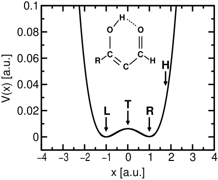
FIG. 1.: The substituted malonaldehyde model system with its corresponding one dimensional potential energy function as given in Eq.(8). L, T, R, H indicate the different wavepacket initial positions utilized for the simulated inversions.

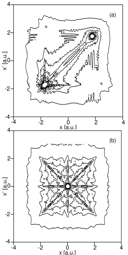
FIG. 2.: Contour plots of the kernel matrices $\textstyle A$. (a) configuration H and (b) configuration T. The numerical values for the matrix entries range from $\thicksim 10^{3}$ on the diagonal to $\thicksim 10^{-8}$ on the boundaries. The contour levels correspond to: 1 (outer line), 31, 61, …, 211.

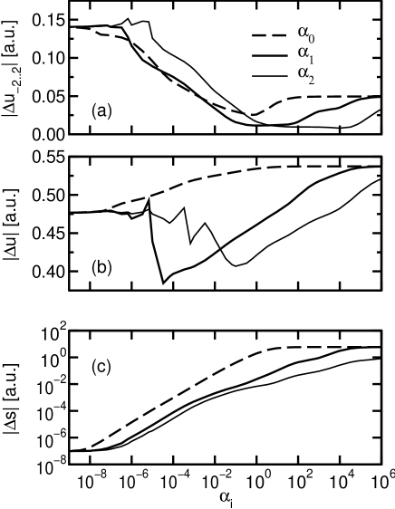
FIG. 3.: $\alpha_{i}$ parameter scans performed with configuration H. Panels (a) and (b) display the solution defect $|\Delta u|$ with respect to two different inversion ranges: $-2\leqslant x\leqslant 2$ and $-4\leqslant x\leqslant 4$, respectively. Panel (c) shows the system defect $|\Delta s|$ for the entire domain $-4\leqslant x\leqslant 4$.

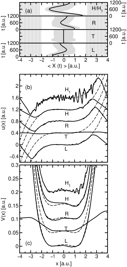
FIG. 4.:

FIG. 4. Extractions of the potential under the conditions given in table II. (a) the time evolution of the position average $\langle x(t)\rangle$ accompanied by the left- and righthand variance (i.e., shaded regions bounded by Eqs.(18) and (19)) to indicate the regions predominantly covered by the probability densities. The grey domains on the extreme left and right mark classically forbidden areas (cf. table I).(b) the reconstructed $u(x)$ and the corresponding potential $V(x)$ in (c) with a suitably chosen additive constant. For comparison the exact solutions are included as dashed lines. The individual curves have been offset for graphical reasons and the detailed presentation of $V(x)$ is restricted to $|x|\lesssim 2.5$ since the boundary regions will not be extracted correctly due to lack of data sampling there.

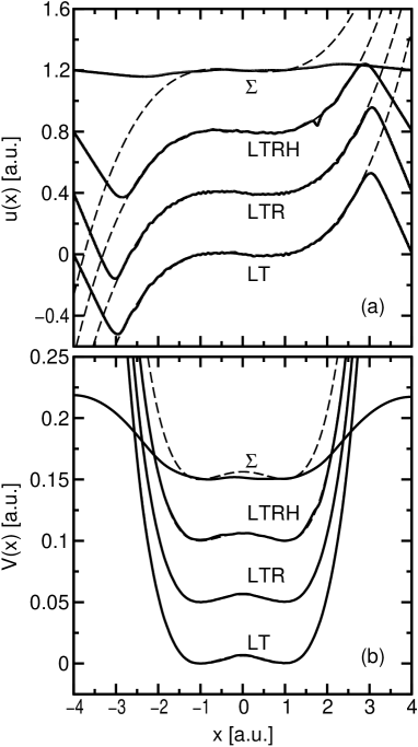
FIG. 5.: Extraction of the PES for optimally combined (LT, LTR, and LTRH) as well as $\rho$-combined data $(\Sigma)$. See the text and table II for details. The curves for the derivative $u(x)$ in (a) and the PES in (b) have been offset for graphical clarity and exact solutions (dashed lines) added for comparison. For optimal combinations of the data the original and reconstructed PES are almost indistinguishable.

REFERENCES

• [1] R. D. Levine and R. B. Bernstein, Molecular Reaction Dynamics (Oxford Univ. Press, New York, N.Y., 1974).
• [2] M. Born and J. R. Oppenheimer, Annalen der Physik 84, 457 (1927).
• [3] D. R. Hartree, Proceedings of the Cambridge Philosophical Society 24, 89 (1928).
• [4] V. A. Fock, Zeitschrift für Physik 61, 126 (1930).
• [5] V. A. Fock, Zeitschrift für Physik 62, 795 (1930).
• [6] A. Szabo and N. S. Ostlund, Modern Quantum Chemistry: Introduction to Advanced Electronic Structure Theory (Macmillan Publishing, New York, 1982).
• [7] P. M. Morse, Physical Review 34, 57 (1929).
• [8] R. B. Gerber, M. Shapiro, U. Buck, and J. Schleusener, Physical Review Letters 41, 236 (1978).
• [9] B. Lowe, M. Pilant, and W. Rundell, SIAM Journal on Mathematical Analysis 23, 482 (1992).
• [10] T.-S. Ho and H. Rabitz, Journal of Physical Chemistry 97, 13447 (1993).
• [11] Quantum Inversion Theory and Applications, edited by H. V. von Geramb (Springer, New York, N.Y., 1994).
• [12] R. Fabiano, R. Knobel, and B. Lowe, IMA Journal or Numerical Analysis 15, 75 (1995).
• [13] D. H. Zhang and J. C. Light, Journal of Chemical Physics 103, 9713 (1995).
• [14] T. Ho, H. Rabitz, S. Choi, and M. Lester, Journal of Chemical Physics 104, 1187 (1996).
• [15] A. Zewail, Journal of Physical Chemistry 97, 12427 (1993).
• [16] M. Shapiro, Journal of Physical Chemistry 100, 7859 (1996).
• [17] J. D. Geiser and P. M. Weber, Journal of Chemical Physics 108, 8004 (1998).
• [18] E. Schrödinger, Annalen der Physik 79, 361 (1926).
• [19] W. Zhu and H. Rabitz, Journal of Chemical Physics 111, 472 (1999).
• [20] W. Zhu and H. Rabitz, Journal of Physical Chemistry A 103, 10187 (1999).
• [21] Z. Vager, R. Naaman, and E. P. Kanter, Science 244, 426 (1989).
• [22] K. Kwon and A. Moscowitz, Physical Review Letters 77, 1238 (1996).
• [23] A. Assion et al., Physical Review A 54, R4605 (1996).
• [24] J. C. Williamson et al., Nature 386, 159 (1997).
• [25] J. L. Krause, K. J. Schafer, M. Ben-Nun, and K. R. Wilson, Physical Review Letters 79, 4978 (1997).
• [26] R. R. Jones, Physical Review A 57, 446 (1998).
• [27] P. Ehrenfest, Zeitschrift für Physik 45, 455 (1927).
• [28] W. Zhu and H. Rabitz, Journal of Physical Chemistry B 104, 10863 (2000).
• [29] A. K. Louis, GAMM-Mitteilungen 1, 5 (1990).
• [30] W. H. Press, S. A. Teukolsky, W. T. Vetterling, and B. P. Flannery, Numerical Recipes in C: The Art of Scientific Computing, 2nd ed. (Cambridge University Press, ADDRESS, 1994).
• [31] N. Došlić, O. Kühn, J. Manz, and K. Sundermann, Journal of Physical Chemistry A 102, 9645 (1998).
• [32] M. D. Feit and J. A. Fleck, Applied Optics 17, 3990 (1978).
• [33] M. D. Feit, J. A. Fleck, and A. Steiger, Journal of Computational Physics 47, 412 (1982).
• [34] A. N. Tikhonov and F. John, in Solutions of Ill-Posed Problems, Scripta Series in Mathematics, edited by V. Arsenin (Winston, Washington, D.C., 1977).
• [35] For $b(x)$, a related issue pointed out in [19] is the stability of $b(x)$ in view of the need to take the second time derivative of the probability density. An approach based on partial integration over time has been proposed calling for a first order time derivative only. However, a check of the inversion performance based on partial integration produced unsatisfactory results. It will always be extremely difficult to reliably compute the terms
$$\left.-\frac{m}{T}\rho(x,t)\,\frac{\text{d}}{\text{d}t}\langle x(t)\rangle\right|_{0}^{T}$$
at only a few $\rho(x,t)$ snapshots in time. One inevitably needs to work with one-sided derivatives at $t=0$ and $T$, which significantly diminishes the accuracy.