Abstract

Fractal behavior and long-range dependence have been observed in an astonishing number of physical systems. Either phenomenon has been modeled by self-similar random functions, thereby implying a linear relationship between fractal dimension, a measure of roughness, and Hurst coefficient, a measure of long-memory dependence. This letter introduces simple stochastic models which allow for any combination of fractal dimension and Hurst exponent. We synthesize images from these models, with arbitrary fractal properties and power-law correlations, and propose a test for self-similarity.

PACS numbers: 02.50.Ey, 02.70-c, 05.40-a, 05.45.Df

I. Introduction. Following Mandelbrot’s seminal essay [1], fractal-based analyses of time series, profiles, and natural or man-made surfaces have found extensive applications in almost all scientific disciplines [2–5]. The fractal dimension, $D$, of a profile or surface is a measure of roughness, with $D\in[n,n+1)$ for a surface in $n$-dimensional space and higher values indicating rougher surfaces. Long-memory dependence or persistence in time series [6–8] or spatial data [9–11] is associated with power-law correlations and often referred to as Hurst effect. Scientists in diverse fields observed empirically that correlations between observations that are far apart in time or space decay much slower than would be expected from classical stochastic models. Long-memory dependence is characterized by the Hurst coefficient, $H$. In principle, fractal dimension and Hurst coefficient are independent of each other: fractal dimension is a local property, and long-memory dependence is a global characteristic. Nevertheless, the two notions are closely linked in much of the scientific literature. This stems from the success of self-similar models such as fractional Gaussian noise and fractional Brownian motion [12] in modeling and explaining either phenomenon. For self-similar processes, the local properties are reflected in the global ones, resulting in the celebrated relationship

$$D=n+1-H$$ (1)

between fractal dimension, $D$, and Hurst coefficient, $H$, for a self-similar surface in $n$-dimensional space [1,3]. Long-memory dependence, or persistence, is associated with the case $H\in(\frac{1}{2},1)$ and therefore linked to surfaces with low fractal dimensions. Rougher surfaces with higher fractal dimensions occur for antipersistent processes with $H\in(0,\frac{1}{2})$. Self-similarity is undoubtedly a natural assumption for many physical, geological, and biological systems. Owing to its intuitive appeal and a lack of suitable alternatives, self-similarity and the linear relationship (1) are believed to be warranted by a large number of real-world data sets.

The stochastic models presented here provide a fresh perspective, since they allow for any combination of fractal dimension, $D$, and Hurst exponent, $H$. The models are very simple, have only two exponents, and allow for the straightforward synthesis of images with arbitrary fractal properties and power-law correlations. We call for a critical assessment of self-similar models and of the relationship (1) through joint measurements of $D$ and $H$ in physical systems.

II. Stationary processes. This section recalls some basic facts for reference below. In the interest of a clear presentation, we restrict ourselves to a discussion of stationary, standard Gaussian [13] random functions $Z(x)$, $x\in\hbox{\zehndoppelt\char 82\relax}^{n}$, which are characterized by their correlation function,

$$c(h)=\;<\!Z(x)Z(x+h)\!>,\qquad\quad h\in\hbox{\zehndoppelt\char 82\relax}^{n}.$$ (2)

The behavior of the correlation function at $h=0$ determines the local properties of the realizations. Specifically, if

$$1-c(h)\sim|h|^{\alpha}\quad\mbox{as}\quad h\to 0$$ (3)

for some $\alpha\in(0,2]$, then the realizations of the random function have fractal dimension

$$D=n+1-\frac{\alpha}{2}$$ (4)

with probability one [14]. Similarly, the asymptotic behavior of the correlation function at infinity determines the presence or absence of long-range dependence. Long-memory processes are associated with power-law correlations,

$$c(h)\sim|h|^{-\beta}\quad\mbox{as}\quad|h|\to\infty,$$ (5)

and if $\beta\in(0,2)$, the behavior is frequently expressed in terms of the Hurst coefficient,

$$H=1-\frac{\beta}{2}.$$ (6)

The asymptotic relationships (3) and (5) can be expressed equivalently in terms of the spectral density and its behavior at infinity and zero, respectively. The traditional stationary, self-similar stochastic process is fractional Gaussian noise [12], that is, the Gaussian process with correlation function

$$c(h)=\frac{1}{2}\left(|h+1|^{2H}-2|h|^{2H}+|h-1|^{2H}\right),\qquad\quad h\in\hbox{\zehndoppelt\char 82\relax},$$ (7)

where $H\in(0,1)$ is the Hurst coefficient. Then $1-c(h)\sim|h|^{2H}$ as $h\to 0$ and

$$\frac{c(h)}{H(2H-1)|h|^{-(2-2H)}}\to 1\quad\mbox{as}\quad|h|\to\infty;$$ (8)

hence, the linear relationship (1) holds with $n=1$. The case $H\in(\frac{1}{2},1)$ is associated with positive correlations, persistent processes, and low fractal dimensions; if $H\in(0,\frac{1}{2})$ we find negative correlations, antipersistent processes, and high fractal dimensions. In other words, the assumption of statistical self-similarity determines the relationships between local and global behavior, or fractal dimension and Hurst effect. By way of contrast, the stochastic models presented hereinafter allow for any combination of fractal dimension and Hurst coefficient.

III. Cauchy class. The Cauchy class consists of the stationary Gaussian random processes $Z(x)$, $x\in\hbox{\zehndoppelt\char 82\relax}^{n}$, with correlation function

$$c(h)=\left(1+|h|^{\alpha}\right)^{-\beta/\alpha},\qquad\quad h\in\hbox{\zehndoppelt\char 82\relax}^{n},$$ (9)

for any combination of the parameters $\alpha\in(0,2]$ and $\beta\geq 0$. It provides flexible power-law correlations and generalizes stochastic models recently discussed and synthesized in geostatistics [15], physics [11,16], hydrology [17], and time series analysis [18–19]. These works consider time series (in discrete time) only, or they restrict $\alpha$ to 1 or 2. The special case $\alpha=2$ has been known as Cauchy model [15], and we refer to the general case, $\alpha\in(0,2]$, as Cauchy class. The correlation function (9) behaves like (3) and (5) as $h\to 0$ and $|h|\to\infty$, respectively. Thus, the realizations of the associated random process have fractal dimension $D$, as given by (4); and if $\beta\in(0,2)$ the Hurst coefficient, $H$, is given by (6). In particular, $D$ and $H$ may vary independently. Figure 1 illustrates two-dimensional realizations of the Cauchy class for various values of $\alpha$ and $\beta$. In each row, $\beta=2-2H$ is constant; but from left to right $\alpha$ increases, that is, the fractal dimension, $D=3-\frac{\alpha}{2}$, decreases. In each column, the fractal dimension is constant, but from top to bottom the Hurst coefficient decreases. These values of $D$ and $H$ are the theoretical quantities as determined by the correlation function. The measured values for the realizations differ from the theoretical ones, due to chance variability and the discrete nature of simulations, but only slightly so. We used the turning bands method with line simulations by the circulant embedding approach [20] to generate the realizations. The code is publicly available [21] and allows, for the first time, for the straightforward synthesis of images with any given combination of fractal dimension and Hurst coefficient.

IV. Modified Cauchy class. The Cauchy class allows for any positive parameter $\beta$ in the power-law (5), and the correlations are always positive. In contrast, fractional Gaussian noise can only model power-laws with $\beta\in(0,2)$, and the correlations eventually become negative if $H\in(0,\frac{1}{2})$ or $\beta\in(1,2)$. We consider the positive correlations to be an advantage of the Cauchy model, since positive power-laws are ubiquitous in the physical, geological, and biological sciences. Nevertheless, we present another stochastic model, the modified Cauchy class, which allows for any combination of fractal dimension and Hurst coefficient and also features the transition from persistence to antipersistence. The modified Cauchy class consists of the stationary Gaussian random processes $Z(x)$, $x\in\hbox{\zehndoppelt\char 82\relax}$, with correlation function

$$c(h)=\left(1+|h|^{\alpha}\right)^{-(\beta/\alpha)-1}\left(1+(1-\beta)|h|^{\alpha}\right),\qquad\quad h\in\hbox{\zehndoppelt\char 82\relax},$$ (10)

where $\alpha\in(0,2]$ and $\beta\geq 0$ [22]. In the same way as (9), the correlation function (10) behaves like (3) and (5) as $h\to 0$ and $|h|\to\infty$, respectively, yielding the same conclusions for the fractal dimension, $D$, given by (4), and Hurst coefficient, $H$, given by (6). Furthermore, there is a transition from positive to negative correlations, or persistence to antipersistence, respectively, depending on whether $\beta$ is smaller or greater than 1. Similarly to fractional Gaussian noise, (10) is a valid correlation function in ℝ, but not in the general Euclidean space $\hbox{\zehndoppelt\char 82\relax}^{n}$ ($n>1$). Figure 2 illustrates realizations of the modified Cauchy class. The graphs along the subdiagonal correspond to parameter combinations with $\alpha+\beta=2$, or $D=2-H$, the same relationship as for self-similar processes. The graphs along the diagonal, however, correspond to parameter combinations of $D$ and $H$ which cannot be realized for self-similar processes.

V. Discussion. We introduced simple stochastic models which separate fractal dimension and Hurst coefficient, and allow for any combination of the two parameters. This is in sharp contrast to traditional, self-similar models for which fractal dimension and Hurst coefficient are linearly related. To our knowledge, Figures 1 provides the first display of fractal images, in which fractal dimension and Hurst coefficient vary independently. Publicly available code [21] allows to synthesize images with any pre-specified combination of fractal dimension and Hurst coefficient. We draw two major conclusions. The first concerns estimation and measurement. Various methods have been proposed and applied to estimate fractal dimension and Hurst coefficient. Popular techniques for estimating or measuring fractal dimension include box-counting, spectral, and increment-based methods [1,3,23–25], and estimators for the Hurst coefficient range from Mandelbrot’s R/S analysis to maximum likelihood [1,7,26]. For estimation of $D$, it is tempting to estimate the Hurst exponent $H$, and then apply the linear relationship (1), or vice versa [27]. We disapprove of any such approach, since the estimator breaks down easily if the critical assumption of self-similarity is violated. Secondly, our findings suggest a straightforward test of self-similarity for time series, profiles, or surfaces [28]: estimate $D$, a local roughness parameter, and $H$, a long-memory parameter, and check whether the estimates are statistically compatible with the linear relationship (1). A positive answer for a large number of data sets, across disciplines, will further substantiate the role of self-similarity within the sciences. Conversely, a negative answer may reject a self-similar model, but it does not preclude fractal statistics or long-memory dependence. The Cauchy and modified Cauchy model provide a striking illustration - and this might be our key point - that the two notions are independent of each other, and can be modeled, explained, and synthesized without recourse to self-similarity.

Figure legends

Figure 1. Realizations of the Cauchy class with $\alpha=0.5,1,2$ (from left to right) and $\beta=0.025,0.2,0.9$ (from top to bottom). In each row, the Hurst coefficient, $H=1-\frac{\beta}{2}$, is constant, but the fractal dimension, $D=3-\frac{\alpha}{2}$, decreases from left to right ($D=2.75,2.5,2$). Accordingly, the images become smoother. In each column, the fractal dimension is held constant, but the Hurst parameter decreases from top to bottom ($H=0.9875,0.9,0.55$). Accordingly, persistence and long-range dependence become less pronounced. The pseudo-random seed is the same for all nine images, and the length of an edge corresponds to a lag of 16 units in the correlation function (9).

Figure 2. Realizations of the modified Cauchy class with $\alpha=0.65$ (left) and $1.95$ (right), and $\beta=0.05$ (top, persistent) and $1.35$ (bottom, antipersistent). Again, the distinct effects of fractal dimension and Hurst coefficient are evident. The pseudo-random seed is the same for all four profiles, and the maximal lag corresponds to 32 units in the correlation function (10).

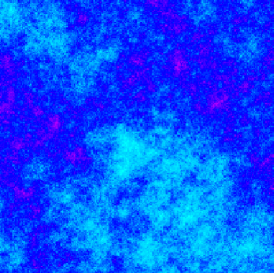
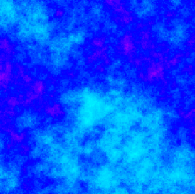
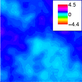
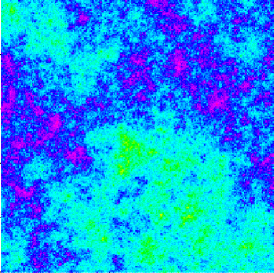
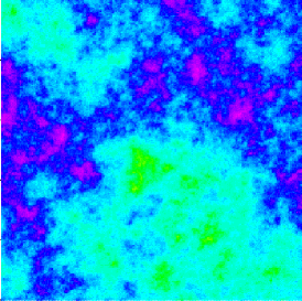
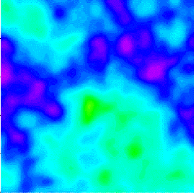
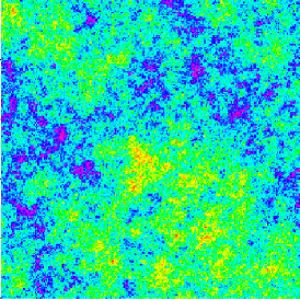
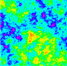
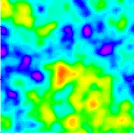
Figure 1: Please use 2 columns.

  

  

Figure 2: Please use 1.5 columns.