Optimal adaptive performance and delocalization in NK fitness landscapes

Abstract

We investigate the evolutionary dynamics of a finite population of sequences adapting to NK fitness landscapes. We find that, unlike in the case of an infinite population, the average fitness in a finite population is maximized at a small but finite, rather than vanishing, mutation rate. The highest local maxima in the landscape are visited for even larger mutation rates, close to a transition point at which the population delocalizes (i.e., leaves the fitness peak at which it was localized) and starts traversing the sequence space. If the mutation rate is increased even further, the population undergoes a second transition and loses all sensitivity to fitness peaks. This second transition corresponds to the standard error threshold transition first described by Eigen. We discuss the implications of our results for biological evolution and for evolutionary optimization techniques.

, , and

1 Introduction

The evolution of a finite population in a rugged, multi-peaked fitness landscape is an important area of research in theoretical biology. Although thoroughly studied over the last 15 years, we are still far from a complete understanding of the intricate dynamics that unfold. Most analytical results deal with very simple fitness landscapes, such as the flat landscape [1], the single peak landscape [2, 3, 4], multiplicative [5, 6] or additive [7] landscapes, or other landscapes that contain a high degree of symmetries, such as the Royal Road landscape [8]. Numerically, one may study more complicated situations, such as RNA folding landscapes [9, 10] or self-replicating computer programs [11]. Here, we are interested in the family of NK landscapes [12, 13]. The NK landscapes are interesting because their ruggedness can be tuned, from a single smooth peak to a completely random landscape, so that the influence of ruggedness on the dynamics of an evolving population can be studied systematically.

Traditionally, NK landscapes have been studied in the context of an adaptive walker, which is essentially a population of size one. If the product of population size $M$ and mutation rate $u$ is small, $uM\ll 1$, the adaptive walk is a reasonable approximation of the full population dynamics. For larger products $uM$, however, quasispecies effects such as error thresholds [14] or selection for mutational robustness [15, 16] are to be expected. Here, we are mainly interested in the change of the population dynamics as the mutation rate is increased, so that $uM$ cannot be considered small.

We investigate the adaptive performance of a finite population on an NK landscape as a function of the mutation rate. Depending on whether we consider the mean population fitness or the maximum fitness in the population, we find different optimal mutation rates. The mean fitness is optimized at a mutation rate that is just sufficiently high to prevent a complete collapse of the population into isogeny (a single genotype). At such a mutation rate, sequence diversity is increased to a value which allows a population to explore the genotype space more efficiently, without losing too much fitness via accumulating deleterious mutations. The maximum fitness, on the other hand, is highest when the mutation rate is so high that the population is on the verge of delocalization. At such a mutation rate, a population is just barely able to maintain the information discovered about the landscape, while at the same time it can explore genotype space at an optimal speed.

2 The NK model

The NK model was introduced by Kauffman [12] in order to study the influence of landscape ruggedness on adaptive evolution. The model is similar to certain physical models of spin-glasses, in particular to the random-energy model [17].

The model is defined as follows. We assume that each organism in the population is composed of $N$ segments, or genes, each of which can be in one of two possible states, designated by 0 or 1. The fitness value of an organisms is then given by the average value of the selective contribution of each of its $N$ genes,

$$F=\frac{1}{N}\sum_{i=1}^{N}f_{i},$$ (1)

where $f_{i}$ denotes the contribution of gene $i$ to the fitness value and is a function of its own state and of the state of $K$ other genes randomly chosen from the remaining $N-1$ ones. The values $f_{i}$ itself are drawn randomly from a uniform distribution on the interval $(0,1]$. All random variables in the NK model are quenched, i.e., they are chosen once at the beginning of a simulation run, and then held fixed. Since the functions $f_{i}$ depend on the state of $K$ different genes at a time, the genes in the NK model are not independent, they interact (i.e., the model assumes epistasis between genes). By changing the number of genes $K$ participating in the epistatic interaction, we can shape the fitness landscape. The parameter $K$ controls the ruggedness of the landscape. For small values of $K$ the landscape is smooth, becoming increasingly rugged for higher values of $K$.

The influence of the parameter $K$ on the ruggedness of the NK landscape can be visualized with the aid of the auto-correlation function, derived in the Appendix:

$$\rho(d)=\frac{(N-K)!(N-d)!}{N!(N-K-d)!}\,.$$ (2)

A fast decay of $\rho(d)$ indicates a high degree of ruggedness, because in that case even sequences that are only a few mutations apart contain hardly any information about each other. If $\rho(d)$ decays slowly, on the other hand, information is preserved over large distances in genotype space, which is only possible if the fitness peaks in the landscape are very broad and smooth. In Fig. 1, we have displayed $\rho(d)$ for $N=32$ and various choices of $K$. We find that for $K=1$, the auto-correlation function decays very slowly, in agreement with a smooth fitness landscape. As $K$ is increased, $\rho(d)$ decays increasingly faster, and the landscape becomes more rugged. In the extreme case of $K=N-1$ (not displayed), $\rho(d)$ decays to zero at $d=1$, indicating that the landscape has become completely random at that point.

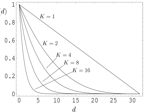
Figure 1: Auto-correlation function in NK landscape with $N=32$.

In order to simulate a population evolving in an NK landscape, we use the following algorithm, which has been used previously by Sibani and Pedersen [18], and is described in detail in Ref. [19]. First, we select 50% of the $M$ sequences in the population for reproduction. An organism is selected with probability proportional to its fitness, so that the most fit individuals contribute most to the composition of the population in the next time step. After reproduction, the population has then reached a size of $1.5M$. Now, we randomly remove one third of the individuals, so that the population after replication and removal consists again of $M$ individuals. The replication mechanism is assumed to be imperfect, and the probability of mutation for a single gene is given by the rate $u$. Recombination is not taken into account in the present work.

3 Results

Our main interest in this work lies in identifying the mutation rate at which a finite population performs “best” in an NK landscape. By “best”, we mean that in equilibrium, and averaged over many independent runs, either the mean or the maximum fitness of the population is maximized. For an infinite population, this question is trivial, since the mean fitness in equilibrium is always maximized at zero mutation rate, and can only decay as the mutation rate increases. For a finite population, however, a mutation rate that is too small leads to a premature standstill in the progress of adaptation, as the population gets trapped in local optima. A mutation rate that is too large, on the other hand, drives the population away from very narrow but high peaks. The optimum mutation rate therefore strikes the right balance between the potential for barrier crossing and the risk of destabilizing fluctuations once a peak has been reached.

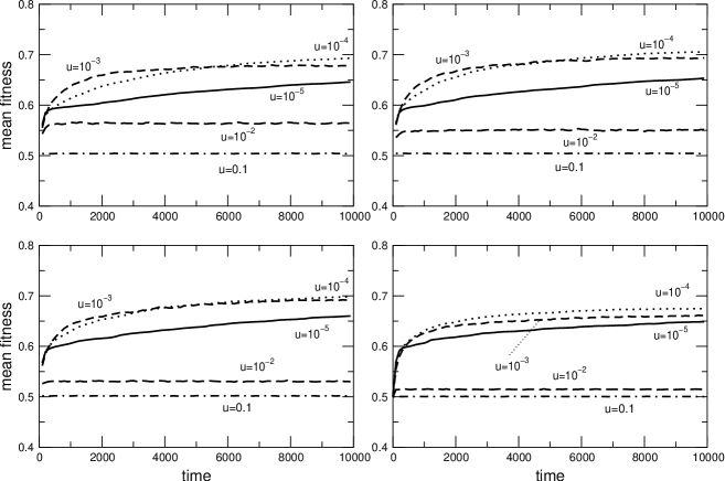
Figure 2: Mean fitness as a function of time, averaged over 50 independent simulation runs, for $N=64$ and $M=5000$. From left to right, and top to bottom, $K=2$, $K=4$, $K=8$, and $K=16$.

Figure 2 shows the mean fitness as a function of time, for various values of $K$ and the mutation rate $u$. The results for different values of $K$ are very similar. We observe an optimal mutation rate (in terms of mean fitness) around $u=10^{-4}$ (a genomic mutation rate of $\mu=Nu=0.0064$). For mutation rates below that value, the mean fitness grows much more slowly. If we increase the mutation rate beyond this value, we find that while the initial adaptation during the first 1,000-2,000 time steps is significantly faster, mean fitness actually drops. This is due to the more efficient exploration of genetic space that a higher mutation rate entails. Initially, when the population starts out in a valley of low fitness, the higher genetic diversity of a population at a higher mutation rate results in more frequent discoveries of higher fitness genotypes. However, when equilibration is reached, the high mutation rate creates a constant influx of deleterious mutations, which reduce the mean fitness in equilibrium.

In order to obtain a more detailed picture of this dynamics, we studied the case of $K=8$ more thoroughly. We recorded mean and maximum fitness after $20,000$ time steps, averaged over 50 independent runs. In addition, we recorded the average Hamming distance to the population’s consensus sequence, in order to obtain a deeper understanding of the population structure that forms at different mutation rates.

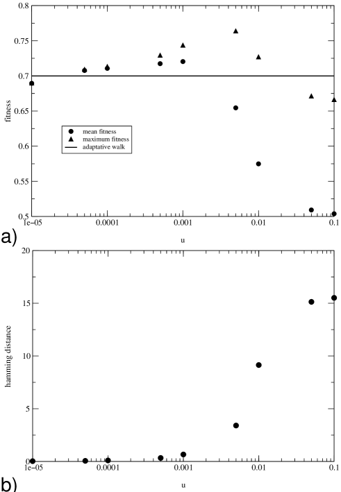
Figure 3: (a) Maximum and mean fitness after 20,000 time steps, averaged over 50 independent runs, as a function of the mutation rate, for $N=32$, $K=8$, and $M=1,000$. (b) Hamming distance to consensus sequence in the same simulations.

Figure 3a) shows mean and maximum fitness in the population as a function of the mutation rate $u$. For comparison, we have also displayed the average height of local maxima in the landscape, obtained as the average over the final fitness of repeated adaptive walks starting from random positions in the landscape. The mean fitness reaches its maximum value around $u=0.001$ ($\mu=0.032$), and the maximum fitness around $u=0.005$ ($\mu=0.16$). At $u=0.1$, the mean fitness has reached the value 0.5, which corresponds to the average fitness of an arbitrary sequence in a NK landscape. At this mutation rate, selection has ceased to have any influence on the population.

For a very low mutation rate, $u=10^{-5}$, we observe that both the mean and the maximum fitness lie below the average height of local maxima in the landscape. However, we expect them to lie exactly on the average height of local maxima in perfect equilibration, because a finite population behaves like an adaptive walker if the mutation rate is sufficiently low. The discrepancy we observe is caused by the finite time of the experiment (20,000 time steps). The lower the mutation rate, the longer it takes until a local maximum is reached, because the rate at which advantageous mutations are discovered is directly proportional to $u$ for small $u$. In the particular case of $u=10^{-5}$, the time allotted for the simulations was not sufficient to allow complete equilibration.

For mutation rates above $u=10^{-4}$, both mean and maximum fitness lie above the height of the local maxima. This demonstrates that a finite population, evolving at the appropriate mutation rate, can perform truly better than an adaptive walk, due to the fact that it can cross fitness barriers in situations where an adaptive walker would simply get stuck in a local sub-optimum.

Figure 3b) shows the mean Hamming distance to the consensus sequence as a function of the mutation rate. For small $u$, we witness the collapse of the population to an isogenic one, reflected in an average Hamming distance of zero. In that regime, the dynamics of the population is only determined by the rate at which advantageous mutations are found, as discussed above. For larger $u$, the Hamming distance between sequences increases. At about $u=0.005$, which is the value at which a population discovers the highest local optima, the average Hamming distance to the consensus sequence is already about three. Beyond $u=0.005$, the Hamming distance increases quickly, until it reaches approximately 16 at $u=0.1$. The value of 16 is exactly half the sequence length $N=32$, which means that the population is completely random at this point. This is in agreement with the mean fitness of 0.5 that we find at this mutation rate. At $u=0.1$, the population transitions from order to disorder. This transition corresponds to the error threshold, which was first observed by Eigen [20], and later found in a large variety of different evolutionary settings [21, 22, 23, 24, 25].

Figure 4: Histogram for the Hamming distance between the sequences in the population and the consensus sequence at time $t=20,000$. In these simulations $M=5000$, $N=32$ and $K=8$. The probability of mutation per digit is: (a) $u=0.001$, (b) $u=0.005$, (c) $u=0.01$ e (d) $u=0.1$.

Figure 4 shows the population structure at various mutation rates in more detail, as a histogram of the sequences’ distances to the consensus sequence. We find that for $u=0.005$, the rate at which the population discovers the highest local optima, the consensus sequence still makes up a significant proportion of the population, although the population’s center has already moved away from the consensus sequence, to a distance of about two. For a slightly higher mutation rate, $u=0.01$, the population’s center moves even further away from the consensus sequence, which in turn is represented by only 1 or 2 % of the sequences in the population or else disappears completely. A more detailed analysis of this regime reveals that in addition to being almost extinct, the consensus sequence also starts to wander about in sequence space. This can be seen in Fig. 5, where we have displayed the average distance to the consensus sequence and the average distance to the consensus sequence of 100 time steps past, as a function of time. While for $u=0.005$ and lower, the two curves lie exactly on top of each other, there are significant deviations between the two curves for larger $u$, which shows that the consensus sequence moves for these mutation rates. However, the population has not yet crossed the error threshold at $u=0.01$, since its structure is still clearly different from complete randomness, and the mean fitness is still above 0.5. Instead it flees the fitness peak it used to inhabit (delocalizes) and settles on many adjacent, most likely “flatter” [26] ones. The population thus undergoes an additional transition prior to experiencing the error threshold. This transition is a purely stochastic effect (i.e., it depends crucially on a finite population size). We will refer to it as the delocalization transition, since the population becomes delocalized and starts to drift through sequence space, re-localizing on adjacent (lower fitness) maxima. A similar transition was previously observed by Bonhoeffer and Stadler [27] in two different landscapes, the Sherrington Kirkpatrick spin glass and the Graph Bi-partitioning landscape, and seems to be a generic finite population effect on rugged fitness landscapes.

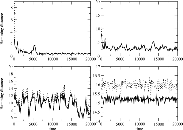
Figure 5: The probability of mutation per digit is: (a) $u=0.001$, (b) $u=0.005$, (c) $u=0.01$ e (d) $u=0.1$.

4 Discussion

In the present work, we have considered both mean and maximum fitness as criteria for optimal adaptive performance. Which one of the two is the more appropriate depends on the context. In biological evolution, the mean population fitness is what determines long-term evolutionary success. A population centered around a particularly high local maximum can easily be driven to extinction if it carries a high load of deleterious mutations and has to compete with another population that has a higher mean, but lower maximum fitness [26]. In evolutionary optimization, on the other hand, we are interested in a single particularly good solution, and the mean fitness is rather meaningless. In that context, optimization of the maximum fitness is more interesting. In the following, we will discuss our results both in the context of biological evolution and evolutionary optimization. We begin with biological evolution.

It has been conjectured by Eigen [28] that optimal adaptation is realized at the verge of the error threshold, and that natural populations should therefore evolve towards the error threshold. Here, we have found that this is clearly not the case in NK landscapes. Rather, the mean fitness (which is the relevant quantity for natural populations, see above) is maximized at mutation rates that generate only a moderate sequence diversity, far away from the error threshold. Maximum rate of evolution also occurs before the error threshold, and before the loss of the consensus sequence. The true error threshold, when sequences diffuse through sequence space without relocalization, occurs at much higher mutation rates, after the consensus sequence is long gone.

The delocalization phase for mutation rates below the error transition corresponds to the situation of Muller’s ratchet in classical population genetics [29, 30]. Muller’s ratchet is a stochastic effect that occurs when either the population size becomes too small, or the mutation rate too high, to sustain a finite population in equilibrium. The population then starts to lose the highest fitness individuals, a process that continues unabated until the population dies out [31]. In contrast to that, here we do not observe a continued loss of fitness, we rather find that the population sustains itself in the neighborhood of high local optima. The difference between our situation and Muller’s ratchet model is that the ratchet model assumes a single peak landscape, where only extremely rare back mutations can compensate for the loss in fitness that the forward mutations carry. In a rugged landscape such as the NK landscape, on the other hand, there are a large number of local optima nearby, which leads to a significant number of compensatory mutations (which, in effect, delocalize the population). Therefore, although the population becomes delocalized, it can nevertheless evade continued fitness loss and extinction.

Let us now discuss the implications of our findings for evolutionary optimization. As we have mentioned above, in evolutionary optimization we are interested in the highest possible maximum fitness in the population. We have found that in NK landscapes, this is realized for mutation rates close to the delocalization transition. This could be utilized for evolutionary optimization in the following way. A number of short initial runs could be used to find the regime in which the delocalization transition takes place. Production runs would then be run at a mutation rate slightly below that regime.

We should also point out that the genomic mutation rates found for the NK landscape are by no means meant to be universal. We expect to find different rates for different fitness landscapes, although we expect the order of events (highest mean fitness, highest maximum fitness, delocalization, error threshold) with increasing mutation rate to remain the same (some of the events may coincide). For example, it is suspected that the mutation rate of RNA viruses is optimal at around $\mu\approx 0.76$ [32] while it appears to be much lower for DNA viruses ($\mu\approx 0.003$ [33]). The optimal rate for finding fitness maxima in the “Royal Road” landscape [34] was found to be of the order of $\mu=0.5$, and around $\mu=1.0$ for digital organisms [11]. In general, optimal rates depend on the supply of advantageous mutations, and on the average height of maxima with respect to random sequences. The presence of a delocalization transition depends on whether or not a fair supply of “secondary” maxima can be found near the initial fitness peak.

It is interesting to compare the delocalization transition of the present work to the behavior of an adaptive walker in a dynamic fitness landscape. In Ref. [35], it was shown that an adaptive walker can traverse the entire sequence space if the fitness landscape is changing slowly. The average fitness encountered on such walks (from peak to peak) lies above the average height of local optima in such landscapes if the landscape changes slowly enough. Here, we find that a population can even traverse a static landscape if the mutation rate is sufficiently high. The local maxima visited by the population (after delocalization) are of similarly high fitness, as can be seen from Fig. 3a) for $u=0.01$. The main difference between the two processes is that the adaptive walker corresponds to a population evolving at a very low mutation rate, such that the mean fitness and the maximum fitness in the population coincide. The high mutation rate necessary for delocalization, on the other hand, implies that the average fitness lies far below the maximum fitness. Therefore, it is unclear to what extent a natural population could utilize these local optima, if at the same time the population has to suffer from a high load of deleterious mutations. Nevertheless, as we have mentioned above, these local optima may present an effective means to halt Muller’s ratchet.

Appendix A Auto-correlation function in NK landscapes

The auto-correlation function $\rho(d)$ at Hamming distance $d$ can be calculated with the following reasoning: we only have to calculate the probability that the fitness contribution of a single gene remains unchanged after $d$ mutations [36]. For $d=1$, this probability is $(N-K)/N$, since there are $N-K$ of the total $N$ genes that will not affect the state of the particular gene we are interested in. For $d=2$, we have then $(N-K)(N-K-1)/[N(N-1)]$, since the second mutation may hit any of the $N-K-1$ genes among the $N-1$ remaining ones. Clearly, for arbitrary $d$, we have

$$\rho(d) = \frac{(N-K)(N-K-1)\dots(N-K-d+1)}{N(N-1)\dots(N-d+1)}$$ (3)

$$= \frac{(N-K)!(N-d)!}{N!(N-K-d)!}\,.$$

Note that this derivation does not depend on whether the $K-1$ interacting genes are chosen randomly (as we assumed throughout the present paper) or as the nearest neighbors of the gene they interact with. Even if all $K$ genes are chosen completely randomly for every $f_{i}$ (the “purely random” version of the NK model), the result remains unaltered.

Equation (3) differs from previously reported results for the autocorrelation function in NK landscapes. In [36], three different functional forms for $\rho(d)$ are reported for the three different types of NK landscapes. Similar results are given in [37, 38, 39]. The results given in [36] for the random neighbor and purely random model are of a very simple functional form, and clearly disagree with Eq. (3). The result for the nearest neighbor model, on the other hand, is more complicated and involves a sum over combinatorial terms. A detailed analysis reveals that the sum can actually be taken, and the resulting expression simplifies to ours. Hence, the previously published correlation function for the nearest neighbor case is correct, though awkward, while the other two cases are incorrect.

References

- [1] B. Derrida and L. Peliti. Evolution in a flat fitness landscape. Bull. Math. Biol., 53:355–382, 1991.
- [2] M. Nowak and P. Schuster. Error thresholds of replication in finite populations—mutation frequencies and the onset of Muller’s ratchet. J. theor. Biol., 137:375–395, 1989.
- [3] P. R. A. Campos and J. F. Fontanari. Finite-size scaling of the quasispecies model. Phys. Rev. E, 58:2664–2667, 1998.
- [4] P. R. A. Campos and J. F. Fontanari. Finite-size scaling of the error threshold transition in finite populations. J. Phys. A, 32:L1–L7, 1999.
- [5] P. G. Higgs and G. Woodcock. The accumulation of mutations in asexual populations and the structure of genealogical trees in the presence of selection. J. Math. Biol., 33:677–702, 1995.
- [6] G. Woodcock and P. G. Higgs. Population evolution on a multiplicative single-peak fitness landscape. J. theor. Biol., 179:61–73, 1996.
- [7] A. Prügel-Bennett. Modelling evolving populations. J. Theor. Biol., 185:81–95, 1997.
- [8] E. van Nimwegen, J. P. Crutchfield, and M. Mitchell. Statistical dynamics of the royal road genetic algorithm. Theoretical Computer Science, 229:41–102, 1999.
- [9] W. Fontana and P. Schuster. Continuity in evolution: on the nature of transitions. Science, 280:1451–1455, 1998.
- [10] M. A. Huynen, P. F. Stadler, and W. Fontana. Smoothness within ruggedness: The role of neutrality in adaptation. Proc. Natl. Acad. Sci. USA, 93(1):397–401, 1996.
- [11] C. Adami. Introduction to Artificial Life. Telos, Springer-Verlag Publishers, Santa Clara, 1998.
- [12] S. A. Kauffman and S. Levin. Towards a general theory of adaptive walks on rugged landscapes. J. of theor. Biol., 128:11–45, 1987.
- [13] S. A. Kauffman. The Origins of Order. Oxford University Press, Oxford, 1992.
- [14] M. Eigen, J. McCaskill, and P. Schuster. The molecular quasi-species. Adv. Chem. Phys., 75:149–263, 1989.
- [15] E. van Nimwegen, J. P. Crutchfield, and M. Huynen. Neutral evolution of mutational robustness. Proc. Natl. Acad. Sci. USA, 96:9716–9720, 1999.
- [16] C. O. Wilke. Adaptive evolution on neutral networks. Bull. Math. Biol, 63:715–730, 2001.
- [17] B. Derrida. Random energy model: An exactly solvable model of disorded systems. Phys. Rev. B, 24:2613–2626, 1981.
- [18] P. Sibani and A. Pedersen. Evolution dynamics in terraced NK landscapes. Europhysics Letters, 48:346–352, 1999.
- [19] A. Pedersen. Evolutionary dynamics. Master’s thesis, Odense Universitet, 1999.
- [20] M. Eigen. Selforganization of matter and the evolution of biological macromolecules. Naturwissenschaften, 58:465–523, 1971.
- [21] J. Swetina and P. Schuster. Self-replication with errors—A model for polynucleotide replication. Biophys. Chem., 16:329–345, 1982.
- [22] P. Tarazona. Error thresholds for molecular quasispecies as phase transitions: From simple landscapes to spin-glass models. Phys. Rev. E, 45:6038–6050, 1992.
- [23] J. Hermisson, H. Wagner, and M. Baake. Four-state quantum chain as a model of sequence evolution. J. Stat. Phys., 102:315–343, 2001.
- [24] S. Franz and L. Peliti. Error threshold in simple landscapes. J. Phys. A—Math. Gen., 30(13):4481–4487, 1997.
- [25] D. Alves and J. F. Fontanari. Error threshold in the evolution of diploid organisms. J. Phys. A—Math. Gen., 30(8):2601–2607, 1997.
- [26] C. O. Wilke, J. L. Wang, C. Ofria, R. E. Lenski, and C. Adami. Evolution of digital organisms at high mutation rate leads to survival of the flattest. Nature, 412:331–333, 2001.
- [27] S. Bonhoeffer and P. F. Stadler. Error thresholds on correlated fitness landscapes. J. theor. Biol., 164:359–372, 1993.
- [28] M. Eigen. The physics of molecular evolution. Chemica Scripta, 26B:13, 1986.
- [29] H. J. Muller. The relation of recombination to mutational advantage. Mut. Res., 1:2–9, 1964.
- [30] J. Felsenstein. The evolutionary advantage of recombination. Genetics, 78:737–756, 1974.
- [31] M. Lynch and W. Gabriel. Mutation load and the survival of small populations. Evolution, 44:1725–1737, 1990.
- [32] J. W. Drake. Mutation rates among rna viruses. Proc. Natl. Acad. Sci. U.S.A., 96:13910–13913, 1999.
- [33] J. W. Drake. A constant rate of spontaneous mutations in dna-based microbes. Proc. Natl. Acad. Sci. U.S.A., 88:7160–7164, 1991.
- [34] E. van Nimwegen. Optimizing evolutionary search: population-size independent theory. Comput. Method Appl. M., 186:171–194, 2000.
- [35] C. O. Wilke and T. Martinetz. Adaptive walks on time-dependent fitness landscapes. Phys. Rev. E, 60:2154–2159, 1999.
- [36] W. Fontana, P. F. Stadler, E. G. Bornberg-Bauer, T. Griesmacher, I. L. Hofacker, M. Tacker, P. Tarazona, E. D. Weinberger, and P. Schuster. RNA folding and combinatory landscapes. Phys. Rev. E, 47:2083–2099, 1993.
- [37] E. D. Weinberger. Local properties of Kauffman’s - model: A tunable rugged energy landscape. Phys. Rev. A, 44:6399–6413, 1991.
- [38] E. D. Weinberger and P. F. Stadler. Why some fitness landscapes are fractal. J. theor. Biol., 163:255–275, 1993.
- [39] P. Schuster and P. F. Stadler. Landscapes: Complex optimization problems and biopolymer structures. Computers Chem., 18:295–314, 1994.