Floquet Scattering and Classical-Quantum correspondence in strong time periodic fields

Abstract

We study the scattering of an electron from a one dimensional inverted Gaussian atomic potential in the presence of strong time periodic electric fields. Using Floquet theory, we construct the Floquet Scattering matrix in the Kramers-Henneberger frame. We compute the transmission coefficients as a function of electron incident energy and find that they display asymmetric Fano resonances due to the electron interaction with the driving field. We find that the Fano resonances are associated with zero-pole pairs of the Floquet Scattering matrix in the complex energy plane. Another way we “probe” the complex spectrum of the system is by computing the Wigner-Smith delay times. Finally we find that the eigenphases of the Floquet Scattering matrix undergo a number of “avoided crossings” as a function of electron Floquet energy, and this number increases with increasing strength of the driving field. These “avoided crossings” appear to be quantum manifestations of the destruction of the constants of motion and the onset of chaos in classical phase space.

PACS numbers: 32.80.-t, 34.50.-s, 03.65.Nk, 05.45.Mt

I Introduction

The development of ultra-high intensity lasers has led to the study of atoms in external time periodic electric fields that are comparable in strength to the electric fields produced by the atomic nucleus. One of the most interesting phenomena observed in these time periodic systems is the stabilization with increasing laser intensity that was predicted theoretically [1, 2, 3] and has been verified experimentally [4, 5].

In previous studies, one dimensional atomic potentials have been used to predict several phenomena in the theory of laser-atom interactions at high laser intensities. Many of these studies were carried out in the context of Floquet theory formulated in the Kramers-Henneberger (K-H) frame of reference [6, 7], which oscillates with a free electron in the time periodic field. Gavrila and Kaminski [1] developed a nonperturbative method to study electron scattering in the presence of strong time-periodic electric fields. Using three dimensional models, Dimou and Faisal [8] as well as Collins and Csanak [8] have studied resonances in laser assisted scattering. Bhatt, Piraux and Burnett [9] in their work on electron scattering from a polarization potential in the presence of strong monochromatic light, argued the appearance of new light-induced quasibound states (resonances) as the field strength is increased. The same phenomenon was later also observed by Bardsley and Comella [10] and Yao and Chu [11] who used the complex coordinate scaling transformation to compute the complex quasibound states in their study of photodetachment from a one-dimensional Gaussian potential. In addition, the same atomic potential was used by Marinescu and Gavrila [12] to compare the predictions of the full Floquet theory with those of the high-frequency Floquet theory (HFFT), using resonance (Siegert) boundary conditions. (The HFFT theory is a version of the Floquet approach adapted to treat the high frequency limit.) Recently, Timberlake and Reichl [13], using the inverted Gaussian potential, studied the phase-space picture of resonance creation and they showed that the light-induced quasibound states are scarred on unstable periodic orbits of the classical motion.

In this paper, we study the scattering of an electron from a short range atomic potential in the presence of a strong time periodic electric field. The atomic potential we consider is the one-dimensional inverted Gaussian potential, a model that has already offered interesting insights into different aspects of the laser-atom interactions [10, 11, 12]. Our goal is to construct the Floquet Scattering matrix ($S$-matrix) using the full Floquet theory formulated in the K-H frame for a strongly driven atomic system. A Floquet Scattering matrix has been constructed by Li and Reichl [14] for periodically driven mesoscopic systems. The Floquet $S$-matrix connects the outgoing propagating modes to the incoming propagating modes and is a unitary matrix which conserves probability. We construct the Floquet $S$-matrix in the K-H frame where we can define asymptotic states.

In section II, we construct the Floquet $S$-matrix in the K-H frame. In section III.A we compute the transmission coefficients and the poles of the Floquet $S$-matrix and find the quasibound states of the atomic system. In section III.B we compute the Wigner-Smith delay times of the scattered electron as a function of the electron incident energy and show that the Wigner-Smith delay times of the scattered electron due to the presence of the quasibound states are of the same order of magnitude as the lifetimes obtained from the poles of the Floquet $S$-matrix. We finish, in section III.C, with a quite interesting observation. When plotting the eigenphases of the unitary Floquet $S$-matrix as a function of the electron’s Floquet energy we find that at certain energies the eigenphases undergo “avoided crossings” that change the eigenphases character completely. We find that the number of “avoided crossings” increases with increasing strength of the time periodic electric field. The “avoided crossings” observed as the strength of the driving field is increased appear to be quantum manifestations of the destruction of the KAM surfaces and the onset of chaos in the classical phase space.

II The Floquet $S$-matrix

A The model

We study the scattering of an electron in the presence of a strong electric field and a short-range atomic potential. The electric field $E(t)=E_{0}\sin(\omega t)$ ($T=\frac{2\pi}{\omega}$ is the period of the field) is treated within the dipole approximation as a monochromatic infinite plane wave linearly polarized along the direction of the incident electron. The Schrödinger equation, in one space dimension $x$, that describes the dynamics of the system is in atomic units (a.u.)

$$i\frac{\partial\Psi(x,t)}{\partial t}=\left({\frac{1}{2}(-i\frac{\partial}{\partial x}-qA(t))^{2}+V(x)}\right)\Psi(x,t),$$ (1)

where V(x) is the inverted Gaussian potential:

$$V(x)=-V_{0}e^{-(x/\delta)^{2}},$$ (2)

and $q$ is the particle charge which for the electron is $q=-1$ a.u.. The electric field is, $E(t)=-\frac{\partial A(t)}{\partial t}$, where $A(t)$ is the vector potential and is given by

$$A(t)=\frac{E_{0}}{\omega}\cos(\omega t).$$ (3)

We use atomic units $(e=\hbar=m=1)$ throughout this paper, except when otherwise indicated.

To construct the Floquet $S$-matrix of the system, we transform to the K-H frame [6, 7]. In the K-H frame there are well defined asymptotic regions and the boundary conditions are expressed in terms of free electron waves. To obtain the wave function in the K-H frame we introduce the unitary transformation [6, 7]

$$\Phi(x,t)=U_{1}U_{2}\Psi(x,t),$$ (4)

where

$$\begin{array}[]{ccc}U_{1}=e^{\frac{iq^{2}}{2}\int_{-\infty}^{t}A^{2}(t^{\prime})dt^{\prime}}&\mbox{and}&U_{2}=e^{-q\int_{-\infty}^{t}A(t^{\prime})\frac{\partial}{\partial x}dt^{\prime}}\end{array}.$$ (5)

$U_{1}$ is a phase transformation to remove the $A^{2}$ term from Eq.(1) while $U_{2}$ is a space translation transformation to the K-H frame. In the K-H frame, the wave function satisfies the following Schrödinger equation

$$i\frac{\partial\Phi(x,t)}{\partial t}=\left(-\frac{1}{2}\frac{\partial^{2}}{\partial x^{2}}+V(x+a(t))\right)\Phi(x,t),$$ (6)

where $a(t)$ is the classical displacement of a free electron from its center of oscillation in the time periodic field $E(t)$, and is given by

$$\begin{array}[]{ccc}a(t)=-q\int_{-\infty}^{t}A(t^{\prime})dt^{\prime}=a_{0}\sin(\omega t)&\mbox{with}&a_{0}=\frac{-qE_{0}}{\omega^{2}}\end{array}.$$ (7)

In Eq.(6), the potential is a periodic function of time, that is $V(x+a(t))=V(x+a(t+T))$. Thus, according to the Floquet theorem [15], Eq.(6) has solutions of the form

$$\Phi_{\mathcal{E}}(x,t)=e^{-i{\mathcal{E}}t}\phi_{\mathcal{E}}(x,t),$$ (8)

where ${\mathcal{E}}$ is the Floquet energy, ${\mathcal{E}}\in[0,\omega)$, and $\phi_{\mathcal{E}}(x,t)$ is a periodic function of time, $\phi_{\mathcal{E}}(x,t)=\phi_{\mathcal{E}}(x,t+T)$. Taking the Fourier expansion of $\phi_{\mathcal{E}}(x,t)$ we obtain

$$\Phi_{\mathcal{E}}(x,t)=e^{-i{\mathcal{E}}t}\sum_{n=-\infty}^{+\infty}\phi_{n}(x)e^{-in\omega t},$$ (9)

where $n$ indicates the Floquet channel. Note that $\phi_{n}(x)$ is also ${\mathcal{E}}$ dependent but we omit the ${\mathcal{E}}$ subscript to simplify notation. The energy $E$ of an incident electron in the K-H frame is related to the Floquet energy through the expression $E={\mathcal{E}}+n\omega$. Next, we Fourier analyze the potential

$$V(x+a(t))=\sum_{n=-\infty}^{+\infty}V_{n}(a_{0};x)e^{-inwt},$$ (10)

where the Fourier components for the inverted Gaussian potential, Eq.(2), can be written as

$$V_{n}(a_{0};x)=\frac{1}{2\pi}\int_{0}^{2\pi}V(x+a(t))e^{in\omega t}d(\omega t)=-V_{0}\frac{i^{n}}{\pi}\int_{0}^{\pi}\cos(n\omega t)e^{-(x+a_{0}\cos(\omega t))^{2}/\delta^{2}}d(\omega t),$$ (11)

see Fig.(1). To be able to construct the Floquet $S$-matrix, the Fourier components $V_{n}(a_{0};x)$ must be smooth functions in the one space dimension $x$ in the K-H frame. This is indeed the case for the inverted Gaussian potential, Eq.(11). Note that in the K-H frame the potential oscillates back and forth along the $x$-axis (laterally) with the period of the external field.

From Eq.(11), we see that the components $V_{n}(\alpha_{0};x)$ of the atomic potential in the limit $x\rightarrow\pm\infty$ tend to zero faster than $1/x$ and we can thus divide the one space dimension $x$ in three regions: the asymptotic regions I, $x\in[x_{0},\infty)$, and III, $x\in(-\infty,-x_{0}]$, where the potential is asymptotically zero; and the scattering region II, $x\in[-x_{0},x_{0}]$, where the potential $V(x+\alpha(t))$ is not zero, see Fig.(2). In the rest of this paper, for brevity, we refer to the potential in asymptotic regions I and III as being zero instead of asymptotically zero. The choice of $x_{0}$ depends on the value of the parameter $\alpha_{0}$. The larger $\alpha_{0}$ is, the further out we have to define the asymptotic regions I and III.

B Floquet solution in the scattering region II

Substituting Eqs.(9) and (10) into Eq.(6) we obtain an infinite system of coupled differential equations [1] for the Floquet components $\phi_{n}(x)$

$$-\frac{1}{2}\frac{d^{2}}{dx^{2}}\phi_{n}(x)+[V_{0}(\alpha_{0};x)-({\mathcal{E}}+n\omega)]\phi_{n}(x)+\sum_{\stackrel{{\scriptstyle l=-\infty}}{{l\neq n}}}^{+\infty}V_{n-l}(\alpha_{0};x)\phi_{l}(x)=0.$$ (12)

Next, we truncate to a finite number of Floquet channels and take $n_{e}$ and $n_{p}$ to be the lower and upper limit of the Floquet channels considered. That is, $n=-n_{e},...,0,...,n_{p}$ and the total number of Floquet channels is given by $N=n_{e}+n_{p}+1$. After truncating, Eq.(12) can be cast in the following matrix form,

$$\mbox{\boldmath$I$}\frac{d^{2}}{dx^{2}}\mbox{\boldmath$\phi$}^{II}(x)=\mbox{\boldmath$M$}(x)\mbox{\boldmath$\phi$}^{II}(x),$$ (13)

where $I$ is the unit $N\times N$ matrix, $\mbox{\boldmath$\phi$}^{II}(x)$ is the $N\times 1$ matrix with elements $\mbox{\boldmath$\phi$}^{II}_{n}(x)=\phi_{n}(x)$ and $\mbox{\boldmath$M$}(x)$ is an $N\times N$ matrix with elements

$$\mbox{\boldmath$M$}_{n,l}(x)=2(V_{n-l}(\alpha_{0};x)-\delta_{n,l}({\mathcal{E}}+n\omega)),$$ (14)

where $\delta_{n,l}$ is the Kronecker delta and $n,l=-n_{e},...,0,...,n_{p}$. The general solution of the second order $N$ coupled differential equations, Eq.(13), can be written as a linear combination of $2N$ linearly independent columns $\mbox{\boldmath$\chi$}_{j}(x)$, with $j=1,...,2N$, as follows

$$\mbox{\boldmath$\phi$}^{II}(x) = c_{1}\mbox{\boldmath$\chi$}_{1}(x)+c_{2}\mbox{\boldmath$\chi$}_{2}(x)+\cdots+c_{N}\mbox{\boldmath$\chi$}_{N}(x)+d_{1}\mbox{\boldmath$\chi$}_{N+1}(x)+d_{2}\mbox{\boldmath$\chi$}_{N+2}(x)+\cdots+d_{N}\mbox{\boldmath$\chi$}_{2N}(x)$$ (15)

$$\equiv \mbox{\boldmath$X$}^{(1)}(x)\mbox{\boldmath$C$}+\mbox{\boldmath$X$}^{(2)}(x)\mbox{\boldmath$D$}$$ (16)

where $\mbox{\boldmath$X$}^{(1)}(x)$ and $\mbox{\boldmath$X$}^{(2)}(x)$ are $N\times N$ matrices whose elements are functions of the one space dimension $x$ and $C$, $D$ are constant $N\times 1$ matrices. Each of the linearly independent columns $\mbox{\boldmath$\chi$}_{j}(x)$ satisfies Eq.(13)

$$\mbox{\boldmath$I$}\frac{d^{2}}{dx^{2}}\mbox{\boldmath$\chi$}_{j}(x)=\mbox{\boldmath$M$}(x)\mbox{\boldmath$\chi$}_{j}(x)\Rightarrow\frac{d^{2}}{dx^{2}}\chi_{n,j}(x)=\sum_{l=-n_{e}}^{n_{p}}\mbox{\boldmath$M$}_{n,l}(x)\chi_{l,j}(x),$$ (17)

where $n=-n_{e},...,0,...,n_{p}$ and $j=1,...,2N$. The functions $\chi_{n,j}(x)$ can be found analytically if the matrix elements of $\mbox{\boldmath$M$}(x)$ are constant. From Eq.(15), it follows that every channel function $\phi_{n}^{II}(x)$ can be written as a linear combination of $2N$ functions $\chi_{n,j}(x)$ and thus, the wavefunction in the scattering region II is given by

$$\Phi^{II}_{\mathcal{E}}(x,t)=\sum_{n=-n_{e}}^{n_{p}}\sum_{m=1}^{N}(\chi_{n,m}(x)c_{m}+\chi_{n,N+m}(x)d_{m})e^{-i{\mathcal{E}}t}e^{-in\omega t}.$$ (18)

C Floquet solution in the asymptotic regions

In the asymptotic regions I and III the potential $V(x+\alpha(t))$ is zero. Thus, we can consider as our boundary conditions a superposition of incoming and outgoing free electron waves in the $N$ truncated Floquet channels that are incident from both sides of the scattering region:

$$\Phi^{I}_{\mathcal{E}}(x,t)=\sum_{n=-n_{e}}^{n_{p}}\phi_{n}^{I}(x)e^{-i{\mathcal{E}}t}e^{-in\omega t}=\sum_{n=-n_{e}}^{n_{p}}b_{n}^{out}\frac{e^{ik_{n}x}}{\sqrt{k_{n}}}e^{-i{\mathcal{E}}t}e^{-in\omega t}+\sum_{n=-n_{e}}^{n_{p}}b_{n}^{in}\frac{e^{-ik_{n}x}}{\sqrt{k_{n}}}e^{-i{\mathcal{E}}t}e^{-in\omega t},$$ (19)

$$\Phi^{III}_{\mathcal{E}}(x,t)=\sum_{n=-n_{e}}^{n_{p}}\phi_{n}^{III}(x)e^{-i{\mathcal{E}}t}e^{-in\omega t}=\sum_{n=-n_{e}}^{n_{p}}a_{n}^{out}\frac{e^{-ik_{n}x}}{\sqrt{k_{n}}}e^{-i{\mathcal{E}}t}e^{-in\omega t}+\sum_{n=-n_{e}}^{n_{p}}a_{n}^{in}\frac{e^{ik_{n}x}}{\sqrt{k_{n}}}e^{-i{\mathcal{E}}t}e^{-in\omega t},$$ (20)

where $b_{n}^{in}$, $a_{n}^{in}$ and $b_{n}^{out}$, $a_{n}^{out}$ are the probability amplitudes of the incoming and outgoing electron waves, respectively, that are incident in the nth Floquet channel with energy $E={\mathcal{E}}+n\omega$, see Fig.(2). Propagating modes are incident on the Floquet channels $n=0,...,n_{p}$ and have wavevectors $k_{n}=\sqrt{2({\mathcal{E}}+n\omega)}$, while evanescent modes occupy the Floquet channels $n=-n_{e},...,-1$ and have imaginary wavevectors $k_{n}=i\sqrt{2|{\mathcal{E}}+n\omega|}$. The current density of the evanescent modes is zero. We note that the terms propagating/evanescent modes correspond to what some authors refer to as open/closed channels, respectively. For the Floquet $S$-matrix to be unitary we need to normalize the current density of the propagating modes. To do so, we have introduced the constants $1/\sqrt{k_{n}}$ in the wavefunction in Eqs.(19) and (20). To simplify notation in Eqs.(19) and (20), we introduce the constants $1/\sqrt{k_{n}}$ for the evanescent modes as well, even though they have zero current density.

It is important to note, once again, that the reason we choose to work in the K-H frame is that in this frame we can define asymptotic regions where the potential is zero and thus, the Floquet channels are not coupled, in contrast with the scattering region, as we have already shown. The existence of the asymptotic regions guarantees that probability is conserved in the truncated number of Floquet channels and thus the Floquet $S$-matrix is a unitary matrix.

D Floquet $S$-matrix

The Floquet $S$-matrix connects the outgoing propagating modes with the incoming propagating modes, and in this section we show how to construct it. As we show in what follows, the Floquet $S$-matrix connects channels with energies that differ by an integer multiple of $\omega$, while in the usual time-independent scattering theory the $S$-matrix connects channels with the same energy. The reason is that the Floquet $S$-matrix describes a time-dependent process and thus the energy of the incident electron is not conserved. However, because the Hamiltonian is time periodic, according to Floquet theory [15], the Floquet energy $\mathcal{E}$ defined modulo $\omega$ is a conserved quantity.

The wavefunction and its first spatial derivative must be continuous at the boundaries of the asymptotic regions $\pm x_{0}$. At $x=x_{0}$ these conditions lead to

$$b_{n}^{out}\frac{e^{ik_{n}x_{0}}}{\sqrt{k_{n}}}+b_{n}^{in}\frac{e^{-ik_{n}x_{0}}}{\sqrt{k_{n}}}=\sum_{m=1}^{N}(\chi_{n,m}(x_{0})c_{m}+\chi_{n,N+m}(x_{0})d_{m}),$$ (21)

$$ik_{n}b_{n}^{out}\frac{e^{ik_{n}x_{0}}}{\sqrt{k_{n}}}-ik_{n}b_{n}^{in}\frac{e^{-ik_{n}x_{0}}}{\sqrt{k_{n}}}=\sum_{m=1}^{N}(\chi^{\prime}_{n,m}(x_{0})c_{m}+\chi^{\prime}_{n,N+m}(x_{0})d_{m}),$$ (22)

where $\chi^{\prime}_{n,m}(x)=\frac{d\chi_{n,m}(x)}{dx}$ and $\chi^{\prime}_{n,N+m}(x)=\frac{d\chi_{n,N+m}(x)}{dx}$, while at $x=-x_{0}$ they lead to

$$a_{n}^{out}\frac{e^{ik_{n}x_{0}}}{\sqrt{k_{n}}}+a_{n}^{in}\frac{e^{-ik_{n}x_{0}}}{\sqrt{k_{n}}}=\sum_{m=1}^{N}(\chi_{n,m}(-x_{0})c_{m}+\chi_{n,N+m}(-x_{0})d_{m}),$$ (23)

$$-ik_{n}a_{n}^{out}\frac{e^{ik_{n}x_{0}}}{\sqrt{k_{n}}}+ik_{n}a_{n}^{in}\frac{e^{-ik_{n}x_{0}}}{\sqrt{k_{n}}}=\sum_{m=1}^{N}(\chi^{\prime}_{n,m}(-x_{0})c_{m}+\chi^{\prime}_{n,N+m}(-x_{0})d_{m}).$$ (24)

Due to the connection conditions Eqs.(21), (22), (23) and(24) only $2N$ out of the $6N$ coefficients are arbitrary and we choose those to be the incoming probability amplitudes $a^{in}$ and $b^{in}$. In Eqs.(21), (22), (23) and(24), the probability amplitudes $a^{in}$ and $b^{in}$ of the evanescent modes are zero because of the unbounded character of the exponentials they multiply in the asymptotic regions I and III. That is, $b_{n}^{in}=a_{n}^{in}=0$, for $n=-n_{e},...,-1$. We now introduce the $N\times N$ matrices

$$\begin{array}[]{lll}(\mbox{\boldmath$K$}_{\pm})_{n,l}=e^{\pm ik_{n}x_{0}}\delta_{n,l},&(\mbox{\boldmath$K$}^{\prime}_{\pm})_{n,l}=\pm ik_{n}e^{\pm ik_{n}x_{0}}\delta_{n,l},&\mbox{$n,l=-n_{e},...,0,...,n_{p},$}\end{array}$$ (25)

$$\mbox{\boldmath$J$}_{n,l}=\left\{\begin{array}[]{ll}0,&\mbox{if $n\neq l$ and if $n=l=-n_{e},...,-1,$}\\ 1,&\mbox{if $n=l=0,...,n_{p}$}\end{array}\right.$$ (26)

and

$$\mbox{\boldmath$\mathcal{N}$}_{n,l}=\begin{array}[]{ccc}\frac{1}{\sqrt{k_{n}}}\delta_{n,l},&&\mbox{$n,l=-n_{e},...,0,...,n_{p}.$}\end{array}$$ (27)

Also $\mbox{\boldmath$X$}^{(1)}_{\pm}\equiv\mbox{\boldmath$X$}^{(1)}(\pm x_{0})$, $\mbox{\boldmath$X$}^{(2)}_{\pm}\equiv\mbox{\boldmath$X$}^{(2)}(\pm x_{0})$, ${\mbox{\boldmath$X$}^{(1)}}^{{}^{\prime}}_{\pm}\equiv{\mbox{\boldmath$X$}^{(1)}}^{{}^{\prime}}(\pm x_{0})$, ${\mbox{\boldmath$X$}^{(2)}}^{{}^{\prime}}_{\pm}\equiv{\mbox{\boldmath$X$}^{(2)}}^{{}^{\prime}}(\pm x_{0})$, where ${\mbox{\boldmath$X$}^{(1)}}^{{}^{\prime}}(x)$ and ${\mbox{\boldmath$X$}^{(2)}}^{{}^{\prime}}(x)$ are the derivatives of $\mbox{\boldmath$X$}^{(1)}(x)$ and $\mbox{\boldmath$X$}^{(2)}(x)$ with respect to the one space dimension $x$. We also introduce the $N\times 1$ matrices $\mbox{\boldmath$A$}_{n}^{out}=a_{n}^{out}$, $\mbox{\boldmath$B$}_{n}^{out}=b_{n}^{out}$, $\mbox{\boldmath$A$}_{n}^{in}=a_{n}^{in}$, $\mbox{\boldmath$B$}_{n}^{in}=b_{n}^{in}$. Next, we write Eqs.(21), (22), (23) and (24) in matrix form as follows

$$\mbox{\boldmath$\mathcal{N}$}\mbox{\boldmath$K$}_{+}\mbox{\boldmath$B$}^{out}+\mbox{\boldmath$\mathcal{N}$}\mbox{\boldmath$K$}_{-}\mbox{\boldmath$J$}\mbox{\boldmath$B$}^{in}=\mbox{\boldmath$X$}^{(1)}_{+}\mbox{\boldmath$C$}+\mbox{\boldmath$X$}^{(2)}_{+}\mbox{\boldmath$D$}$$ (28)

$$\mbox{\boldmath$\mathcal{N}$}\mbox{\boldmath$K$}^{\prime}_{+}\mbox{\boldmath$B$}^{out}+\mbox{\boldmath$\mathcal{N}$}\mbox{\boldmath$K$}^{\prime}_{-}\mbox{\boldmath$J$}\mbox{\boldmath$B$}^{in}={\mbox{\boldmath$X$}^{(1)}}^{{}^{\prime}}_{+}\mbox{\boldmath$C$}+{\mbox{\boldmath$X$}^{(2)}}^{{}^{\prime}}_{+}\mbox{\boldmath$D$}$$ (29)

$$\mbox{\boldmath$\mathcal{N}$}\mbox{\boldmath$K$}_{+}\mbox{\boldmath$A$}^{out}+\mbox{\boldmath$\mathcal{N}$}\mbox{\boldmath$K$}_{-}\mbox{\boldmath$J$}\mbox{\boldmath$A$}^{in}=\mbox{\boldmath$X$}^{(1)}_{-}\mbox{\boldmath$C$}+\mbox{\boldmath$X$}^{(2)}_{-}\mbox{\boldmath$D$}$$ (30)

$$-\mbox{\boldmath$\mathcal{N}$}\mbox{\boldmath$K$}^{\prime}_{+}\mbox{\boldmath$A$}^{out}-\mbox{\boldmath$\mathcal{N}$}\mbox{\boldmath$K$}^{\prime}_{-}\mbox{\boldmath$J$}\mbox{\boldmath$A$}^{in}={\mbox{\boldmath$X$}^{(1)}}^{{}^{\prime}}_{-}\mbox{\boldmath$C$}+{\mbox{\boldmath$X$}^{(2)}}^{{}^{\prime}}_{-}\mbox{\boldmath$D$}$$ (31)

After algebra given in Appendix A we find the Floquet $S$-matrix, that connects the outgoing probability amplitudes of the propagating modes to the incoming probability amplitudes of the propagating modes, to be

$$\left(\begin{array}[]{c}\mbox{\boldmath$A$}_{p}^{out}\\ \mbox{\boldmath$B$}_{p}^{out}\end{array}\right) = \left(\begin{array}[]{cc}\mbox{\boldmath$\mathcal{N}$}_{pp}^{-1}\mbox{\boldmath$r$}_{pp}^{\prime}\mbox{\boldmath$\mathcal{N}$}_{pp}&\mbox{\boldmath$\mathcal{N}$}_{pp}^{-1}\mbox{\boldmath$t$}_{pp}\mbox{\boldmath$\mathcal{N}$}_{pp}\\ \mbox{\boldmath$\mathcal{N}$}_{pp}^{-1}\mbox{\boldmath$t$}_{pp}^{\prime}\mbox{\boldmath$\mathcal{N}$}_{pp}&\mbox{\boldmath$\mathcal{N}$}_{pp}^{-1}\mbox{\boldmath$r$}_{pp}\mbox{\boldmath$\mathcal{N}$}_{pp}\end{array}\right)\left(\begin{array}[]{c}\mbox{\boldmath$A$}_{p}^{in}\\ \mbox{\boldmath$B$}_{p}^{in}\end{array}\right)$$ (38)

$$\equiv \left(\begin{array}[]{cc}\mbox{\boldmath$R$}^{\prime}&\mbox{\boldmath$T$}\\ \mbox{\boldmath$T$}^{\prime}&\mbox{\boldmath$R$}\end{array}\right)\left(\begin{array}[]{c}\mbox{\boldmath$A$}_{p}^{in}\\ \mbox{\boldmath$B$}_{p}^{in}\end{array}\right)\equiv\mbox{\boldmath$S$}\left(\begin{array}[]{c}\mbox{\boldmath$A$}_{p}^{in}\\ \mbox{\boldmath$B$}_{p}^{in}\end{array}\right),$$ (45)

where the $n_{p}+1\times n_{p}+1$ ($n_{p}+1$ is the number of the propagating modes) matrices $\mbox{\boldmath$r$}^{\prime}_{pp}$, $\mbox{\boldmath$r$}_{pp}$, $\mbox{\boldmath$t$}^{\prime}_{pp}$ and $\mbox{\boldmath$t$}_{pp}$ defined in Eqs.(62) and (66) of Appendix A connect propagating modes to propagating modes and contain the evanescent mode effect as is shown in Appendix A. Also the $n_{p}+1\times 1$ matrices $\mbox{\boldmath$A$}^{in}_{p}$ $\mbox{\boldmath$A$}^{out}_{p}$, $\mbox{\boldmath$B$}^{in}_{p}$ and $\mbox{\boldmath$B$}^{out}_{p}$ have elements the amplitudes of the propagating modes and are defined in Eq.(67) of Appendix A, and the $n_{p}+1\times n_{p}+1$ matrix $\mbox{\boldmath$\mathcal{N}$}_{pp}$ has elements the normalization constants of the propagating modes and is defined in Eq.(67) of Appendix A. The matrices $\mbox{\boldmath$R$}^{\prime}$, $R$, $\mbox{\boldmath$T$}^{\prime}$ and $T$ have dimensions $n_{p}+1\times n_{p}+1$ and their elements are given in terms of the elements of the $\mbox{\boldmath$r$}^{\prime}_{pp}$, $\mbox{\boldmath$r$}_{pp}$, $\mbox{\boldmath$t$}^{\prime}_{pp}$ and $\mbox{\boldmath$t$}_{pp}$ matrices as follows

$$\begin{array}[]{cccc}R^{\prime}_{n^{\prime},n}=\sqrt{\frac{k_{n^{\prime}}}{k_{n}}}(\mbox{\boldmath$r$}^{\prime}_{pp})_{n^{\prime},n},&R_{n^{\prime},n}=\sqrt{\frac{k_{n^{\prime}}}{k_{n}}}(\mbox{\boldmath$r$}_{pp})_{n^{\prime},n},&T^{\prime}_{n^{\prime},n}=\sqrt{\frac{k_{n^{\prime}}}{k_{n}}}(\mbox{\boldmath$t$}^{\prime}_{pp})_{n^{\prime},n},&T_{n^{\prime},n}=\sqrt{\frac{k_{n^{\prime}}}{k_{n}}}(\mbox{\boldmath$t$}_{pp})_{n^{\prime},n}\end{array},$$ (46)

with $n^{\prime},n=0,...,n_{p}$.

In Appendix B we show how to obtain numerically the matrices $\mbox{\boldmath$r$}_{pp}$ and $\mbox{\boldmath$t$}_{pp}$. The Floquet $S$-matrix has dimensions $2(n_{p}+1)\times 2(n_{p}+1)$, see Eq.(38), and is determined by the reflection and transmission amplitudes, $R^{\prime}_{n^{\prime},n}$, $R_{n^{\prime},n}$, $T^{\prime}_{n^{\prime},n}$ and $T_{n^{\prime},n}$, of the propagating modes. The elements $|R_{n^{\prime},n}|^{2}$ and $|T_{n^{\prime},n}|^{2}$ are the reflection and transmission coefficients respectively for an electron wave incident on the propagating channel $n$ from the right that gets scattered to the propagating channel $n^{\prime}$, while the elements $|R^{\prime}_{n^{\prime},n}|^{2}$ and $|T^{\prime}_{n^{\prime},n}|^{2}$ are the reflection and transmission coefficients respectively for an electron wave incident on the propagating channel $n$ from the left that gets scattered to the propagating channel $n^{\prime}$.

In this section we have shown how to construct the Floquet $S$-matrix in the K-H frame. The reason we work in the K-H frame is that we can define asymptotic regions where the wavefunction is a superposition of free electron waves. That guarantees that the truncated Floquet $S$-matrix is a unitary matrix, that is, the following condition is satisfied

$$\sum_{n^{\prime}=0}^{n_{p}}[|R_{n^{\prime},n}|^{2}+|T_{n^{\prime},n}|^{2}]=1,$$ (47)

for every incident propagating mode $n=0,...,n_{p}$. The above condition is a statement of conservation of probability. Also, the Floquet $S$-matrix we construct in the K-H frame is isospectral with the corresponding matrix in the Lab frame since a unitary transformation is used to transform from the Lab to the K-H frame, see section II.A. Finally, the criterion we use to successfully truncate to $N$ Floquet channels is that an electron wave incident on the last propagating Floquet channel $n=n_{p}$ is not affected by the scattering potential. That is, the transmission coefficient $|T_{n_{p},n_{p}}|^{2}$ should be equal to one as a function of electron incident energy $E$ ( $E={\mathcal{E}}+n_{p}\omega$) as we discuss in more detail in section III.B.

E Symmetries of the Floquet $S$-matrix

The Hamiltonian of the scattering model we consider in the K-H frame, Eq.(6), is invariant under the transformation $x\rightarrow-x$ and $t\rightarrow t+T/2$, which is known as Generalized Parity. Thus, $H(x,t)=H(-x,t+T/2)$ and therefore $\Phi(-x,t+T/2)$ is also a solution of Eq.(6). Applying the transformation $x\rightarrow-x$ and $t\rightarrow t+T/2$ to Eqs.(19) and (20) it is easy to show that the Floquet $S$-matrix has the following symmetry:

$$\begin{array}[]{cccc}R^{\prime}_{n^{\prime},n}=R_{n^{\prime},n}(-1)^{n^{\prime}-n},&T^{\prime}_{n^{\prime},n}=T_{n^{\prime},n}(-1)^{n^{\prime}-n},&\mbox{with}&n^{\prime},n=0,...,n_{p}\end{array}.$$ (48)

Thus, if we know the reflection/transmission amplitudes, $R_{n^{\prime},n}/T_{n^{\prime},n}$ for electron waves incident from the right using Eqs.(48) we can find the reflection/transmission amplitudes, $R^{\prime}_{n^{\prime},n}/T^{\prime}_{n^{\prime},n}$ for electron waves incident from the left and vise versa.

III Results

In this section, the calculations are performed with the values $V_{0}=0.27035$ a.u. and $\delta=2$ a.u. assigned to the parameters of the inverted Gaussian potential. For these parameters the Gaussian potential supports only one bound state of energy $E_{b}=-0.1327$ a.u. in the field-free case. The parameters $V_{0}$ and $\delta$ were chosen so as to describe the behavior of a one-dimensional model negative chlorine ion, $Cl^{-}$, in the presence of a laser field, and are the same as considered in [11, 12, 16]. The frequency of the time periodic field is taken constant and equal to $\omega=0.236$ a.u. for all our calculations. For these values of the parameters $V_{0}$, $\delta$ and $\omega$ the inverted Gaussian potential has been shown to exhibit stabilization [11, 12].

A Transmission resonances

In this section, we compute the transmission coefficient ${\mathit{T_{n}}}$ and the total transmission coefficient $\mathit{T_{tot,n}}$ as a function of the electron incident energy $E$, where

$$\begin{array}[]{ccccc}{\mathit{T_{n}}}(E)=|T_{n,n}|^{2},&&{\mathit{T_{tot,n}}}(E)=\sum_{n^{\prime}=0}^{n_{p}}|T_{n^{\prime},n}|^{2},&&\mbox{$E\in[n\omega,(n+1)\omega)$}\end{array}$$ (49)

with $n=0,1$. Thus, we consider an electron wave incident from the right with energy $E\in[0,2\omega)$ and compute the transmission coefficients. Keeping the frequency of the time periodic field constant, $\omega=0.236$ a.u., and varying the strength of the driving field, $a_{0}$, we plot the transmission coefficients $\mathit{T_{n}}$ and $\mathit{T_{tot,n}}$ in Figs.(3), (4) and (5) for $\alpha_{0}$ equal to $0.5$, $2.25$ and $5.25$, respectively. The frequency of the driving field $\omega=0.236$ a.u. is chosen so that it is larger than the binding energy of the ground state $|E_{b}|=|-0.1327|$ a.u. in the field-free case. The Floquet channels we retain to obtain the numerical results presented in sections III.A and III.B are $n=-6,...,0,...,6$ for $\alpha_{0}=0.5$, $n=-12,...,0,...,12$ for $\alpha_{0}=2.25$ and $n=-19,...,0,...,19$ for $\alpha_{0}=5.25$, for reasons we discuss in detail at the end of section III.B.

The transmission coefficients $\mathit{T_{n}}$ and $\mathit{T_{tot,n}}$ display sharp asymmetric resonances, as a function of electron incident energy $E$, that involve a dip or a transmission peak/dip as is shown in Figs.(3), (4) and (5). These asymmetric resonances are due to the interaction of the incident electron wave with the laterally oscillating potential in the K-H frame and are the so-called Fano [17, 18] type transmission resonances that are known to occur when a bound state is coupled to a continuum of states. This is indeed the case for the scattering model we consider, where the bound state of the inverted Gaussian potential is coupled to a continuum of states through the time periodic electric field. Note in Figs.(3), (4) and (5) that the difference between the transmission coefficient $\mathit{T_{n}}$ and $\mathit{T_{tot,n}}$ becomes more prominent with increasing $\alpha_{0}$. The reason is that as $\alpha_{0}$ is increased more Floquet channels interfere with the incident electron wave and significantly contribute to the total transmission coefficient. A comparison of Fig.(3) with Figs.(4) and (5) reveals that as the driving field is increased the higher order resonances, for $E>\omega$, become stronger.

We now focus on the transmission coefficient $\mathit{T_{n}}$ and discuss how it “probes” the quasibound states of the system. For $\alpha_{0}=0.5$, see Fig.(3a) the system has only one Fano transmission resonance which for small amplitude of the driving field is associated with the $n=-1$ localized Floquet evanescent mode which has its origin in the bound state of the undriven system. When the strength of the driving field is increased, $\mathit{T_{n}}$ has a second Fano transmission resonance at a higher incident energy, see Figs.(4a) and (5a). This second resonance appears for $a_{0}>1$, as was shown in [11, 12], and it is thus a field induced resonance.

The Fano-resonances, which are indicated by a dip or a transmission peak/dip in the coefficient $\mathit{T_{n}}$, correspond to quasibound states of the system that show up as poles of the Floquet $S$-matrix in the complex energy plane. In what follows, we compute the poles of $\mathit{T_{n}}$ in the complex energy plane. Other elements of the Floquet $S$-matrix have poles as well. As was noted in [19] the asymmetric Fano line shape in $\mathit{T_{n}}$ is associated with zero-pole pairs when plotting $\mathit{T_{n}}$ in the complex energy plane. By a zero-pole pair we mean that every transmission zero of $\mathit{T_{n}}$ along the real energy axis is associated with a pole of $\mathit{T_{n}}$ on the lower half complex energy plane due to the unitarity of the Floquet $S$-matrix [19]. For $\alpha_{0}=0.5$ there is only one zero-pole pair associated with the single transmission resonance seen in $\mathit{T_{n}}$, while for $\alpha_{0}=2.25$ there is a zero-pole pair for each of the two resonances, see Figs.(4a) and (6). For small strengths of the driving field, $\alpha_{0}=0.5$, the location of the pole on the lower half complex energy plane and of the zero on the real energy axis is the same, while there is a small difference for stronger fields, $\alpha_{0}=2.25$. That is why, we can only approximately determine the real part of the quasibound states from the transmission zeros. From the poles in the complex energy plane, we find the real part of the quasibound states to be $Re(E_{1})=0.106$, for $\alpha_{0}=0.5$, and $Re(E_{1})=0.145$, $Re(E_{2})=0.226$, for $\alpha_{0}=2.25$.

The lifetime, $\tau_{L}$ of the quasibound states is determined from the imaginary part of the complex energy, $Im(E)$, where the pole is found. Then

$$\tau_{L}=\frac{1}{\Gamma},$$ (50)

where $\Gamma=2Im(E)$ is the ionization rate. For the inverted Gaussian potential it has been found that with increasing strength of the driving field the ionization rate decreases in an oscillatory manner [11, 12]. In Figs.(7) and (8) we show how the real and imaginary part of the quasibound state energies change as a function of $\alpha_{0}$, for $\alpha_{0}$ ranging from $0$ to $6$ a.u.. The incident particle can emit a photon and drop to a localized Floquet evanescent state. It is in this sense that in Fig.(7) we plot the real part of the quasibound state minus a photon energy and obtain results in agreement with those obtained in [11, 12].

B Wigner-Smith delay times

Wigner’s [20] one dimensional analysis on time delay in a quantum mechanical scattering problem was generalized to multi-channel scattering by Smith [21] who introduced the Hermitian matrix

$$\hat{Q}=i\hat{S}\frac{d\hat{S}^{\dagger}}{dE}$$ (51)

and interpreted its diagonal elements $\mbox{\boldmath$Q$}_{nn}$ as the average delay experienced by a particle incident on the nth channel ($S$ is the unitary scattering matrix).

In what follows, we compute the diagonal elements of the Wigner-Smith delay matrix $Q$ for the system currently under consideration. We first obtain the eigenvalues and eigenvectors of the Floquet $S$-matrix, see Eq.(38), which is a $2(n_{p}+1)\times 2(n_{p}+1)$ matrix when the system is truncated to $n_{p}+1$ propagating modes. The $2(n_{p}+1)$ eigenvalues of the unitary Floquet $S$-matrix have unit magnitude and can thus be cast in the form $e^{i\theta_{i}({\mathcal{E}})}$, where $i=1,...,2(n_{p}+1)$ and $\theta_{i}(\mathcal{E})$ is the ith eigenphase as a function of the Floquet energy $\mathcal{E}$. The eigenvector corresponding to the ith eigenvalue $e^{i\theta_{i}}$ is denoted by $|\theta_{i}>$. We note that the transmission coefficients $\mathit{T_{n}}$ and $\mathit{T_{tot,n}}$ (see section III.A) as well as the Wigner-Smith delay times $\tau_{ws}^{n}$, defined in what follows, are a function of incident electron energy $E\in[0,(n_{p}+1)\omega)$. However, the eigenphases $\theta_{i}$ and the eigenvectors $|\theta_{i}>$ of the Floquet $S$-matrix are a function of the Floquet energy ${\mathcal{E}}\in[0,\omega)$ in the sense that if the Floquet energy is defined as the incident electron energy at a higher propagating channel one finds the exact same eigenvalues and eigenvectors. The Floquet $S$-matrix can be written as

$$\hat{S}=\sum_{i=1}^{2(n_{p}+1)}|\theta_{i}>e^{i\theta_{i}}<\theta_{i}|.$$ (52)

Each of the eigenvectors $|\theta_{i}>$ can be expanded in terms of the propagating free electron waves $|k_{n}>$ that we have used to construct the Floquet $S$-matrix, where $<x|k_{n}>=e^{ik_{n}x}$. That is, $|\theta_{i}>=\sum_{n=0}^{2n_{p}+1}p_{n,i}|k_{n}>$ where $p_{n,i}=<k_{n}|\theta_{i}>$ and $P_{n,i}=|p_{n,i}|^{2}$ is the occupation probability of the $|\theta_{i}>$ eigenvector on the $|k_{n}>$ propagating channel and $n=0,...,n_{p}$ for the right propagating modes and $n=n_{p}+1,...,2n_{p}+1$ for the left propagating modes. The occupation probability of the $|\theta_{i}>$ eigenvector on a mode incident from the right is the same with that of the corresponding mode incident from the left, that is, $P_{n,i}=P_{n+n_{p}+1,i}$ for $n=0,...,n_{p}$. Finally, for each eigenvector $|\theta_{i}>$ the total occupation probability is normalized to 1, $\sum_{n=0}^{2n_{p}+1}P_{n,i}=1$, where modes incident from the right and the left are taken into account. For modes only incident from the right the normalization for the occupation probability takes the form $\sum_{n=0}^{n_{p}}P_{n,i}=0.5$. From Eqs. (51) and (52) and the fact that the eigenvectors $|\theta_{i}>$ form a complete set (the Floquet $S$-matrix is unitary) one can show that

$$<k_{n}|\hat{Q}|k_{n}>\equiv\tau_{ws}^{n}=\sum_{i=1}^{2(n_{p}+1)}\frac{d\theta_{i}}{d{\mathcal{E}}}<k_{n}|\theta_{i}><\theta_{i}|k_{n}>\Rightarrow\tau_{ws}^{n}=\sum_{i=1}^{2(n_{p}+1)}P_{n,i}\frac{d\theta_{i}}{d{\mathcal{E}}}.$$ (53)

The Wigner-Smith delay times $\tau_{ws}^{n}$ are the average times an electron incident on the nth channel with energy $E\in[n\omega,(n+1)\omega)$ is delayed due to its interaction with the laterally oscillating time periodic potential in the K-H frame. The Wigner-Smith delay times for propagating modes incident from the right are the same with those incident from the left, that is, $\tau_{ws}^{n}=\tau_{ws}^{n+n_{p}+1}$ for $n=0,...,n_{p}$.

In Figs.(9), (10) and (11) we plot the Wigner-Smith delay times for $\alpha_{0}$ equal to $0.5$, $2.25$ and $5.25$, respectively, for modes incident from the right. In Table I we compare the Wigner-Smith delay times $\tau_{ws}^{n}$ obtained from the Floquet $S$-matrix with the lifetime $\tau_{L}$ obtained from the poles of the ${\it{T_{n}}}$ transmission coefficient in the complex energy plane and find them to be of the same order of magnitude [22]. At the transmission resonances, the incident electron wave gets trapped by the oscillating potential, populating the quasibound states of the system. The delay of the incident electron wave at the transmission resonances shows up as peaks when plotting the Wigner-Smith delay times as a function of the electron incident energy. Note that as $\alpha_{0}$ increases from $2.25$ to $5.25$ the Wigner-Smith delay time of the 1st quasibound state increases, evidence of stabilization. Another interesting observation is that for small incident energy $E$ the electron has positive Wigner-Smith delay times, for $\alpha_{0}=0.5$, but the electron has negative Wigner-Smith delay times for strong driving fields $\alpha_{0}=2.25$ and $5.25$. These last can arise physically either from reflection of the incident electron before it enters the scattering region or from its acceleration and swift passage through the negative potential [21]. In addition, from Figs.(9), (10) and (11) we see, as expected, that when the electron is incident on higher Floquet channels it delays less and less until for very high energies it is not affected by the potential and the delay time is zero.

Now, let us briefly comment on the truncation error of our numerical calculations. The number of Floquet channels $N$ was chosen for each value of $\alpha_{0}$ so that the error due to truncation remains small. The truncation error for the elements $R_{n^{\prime},n}/T_{n^{\prime},n}$, where $n^{\prime},n=0,...,n_{p}$, is smaller for $n=0$ and it increases as $n$ approaches $n_{p}$, where $n_{p}$ is the last propagating mode and thus the mode with the larger electron incident energy. Thus, the truncation error for the transmission coefficients $\mathit{T_{n}}$ and $\mathit{T_{tot,n}}$ computed in section III.A is smaller than the error for the Wigner-Smith delay times computed in this section. An estimate of the truncation error is given by $1-|T_{n_{p},n_{p}}|^{2}$ as a function of incident electron energy. In all our calculations the truncation error is kept in the order of $10^{-4}$ for $a_{0}=0.5,2.25$ and $10^{-3}$ for $a_{0}=5.25$ so that our results are reliable. As we increase $\alpha_{0}$ we need to consider a larger number of Floquet channels $N$ to maintain a small truncation error in our numerical calculations making it computationally challenging to compute the Wigner-Smith delay times for large values of $\alpha_{0}$.

C Classical-Quantum Correspondence

When we plot the eigenphases of the Floquet $S$-matrix as a function of the electron Floquet energy ${\mathcal{E}}$ we notice that the eigenphases undergo an increasing number of “avoided crossings” with increasing strength $\alpha_{0}$ of the driving field, see Figs.(12), (14), and (15). As we show in what follows, we believe that these “avoided crossings” are a quantum manifestation of chaos in the classical phase space.

Let us explain what we mean by the term “avoided crossing” in terms of the occupation probabilities, $P_{n,i}$, (defined in section III.B) of the $|\theta_{i}>$ eigenvector on the $|k_{n}>$ propagating channel. In what follows we consider the occupation probabilities only for modes incident from the right, that is, $n=0,...,n_{p}$. In Fig.(12) the eigenphases $\theta_{1}$ and $\theta_{2}$ undergo a repulsion when the Floquet energy is equal to the transmission resonance, ${\mathcal{E}}=0.106$, for $\alpha_{0}=0.5$. For very small values of $\alpha_{0}$ the eigenphases cross each other without repelling. It is only as we increase the strength of the driving field that the eigenphases undergo a repulsion which we refer to as an “avoided crossing”. We describe quantitatively the “avoided crossing” between the eigenphases $\theta_{1}$ and $\theta_{2}$ in terms of occupation probabilities. In Fig.(13a) we plot the occupation probabilities $P_{0,1}$, $P_{1,1}$ and $P_{2,1}$ of the $|\theta_{1}>$ eigenvector on the propagating channels n=0,1,2 and in Fig.(13b) we plot the occupation probabilities $P_{0,2}$, $P_{1,2}$ and $P_{2,2}$ of the $|\theta_{2}>$ eigenvector on the propagating channels n=0,1,2 as a function of Floquet energy ${\mathcal{E}}$. Before the “avoided crossing”, ${\mathcal{E}}<0.106$, $|\theta_{1}>$ has support mainly on the second propagating channel, $P_{1,1}\approx 0.5$, and $|\theta_{2}>$ on the first propagating channel, $P_{0,2}\approx 0.5$, while after the “avoided crossing”, ${\mathcal{E}}>0.106$, $|\theta_{1}>$ has support mainly on the first propagating channel, $P_{0,1}\approx 0.5$, and $|\theta_{2}>$ on the second propagating channel, $P_{1,2}\approx 0.5$. This total exchange of character is what we refer to as a sharp “avoided crossing”. Note that for $\alpha_{0}=0.5$ the propagating channels involved in the “avoided crossing” are mainly $n=0,1$. As the strength of the driving field $\alpha_{0}$ is increased an increasing number of propagating channels undergo “avoided crossings”, as shown in Tables II and III.

For increased strength of the driving field the number of avoided crossings increases, see Figs.(14), (15) and it can be that more than two eigenphases participate in an “avoided crossing” for a certain Floquet energy. For example, this is the case for the “avoided crossing” at ${\mathcal{E}}\approx 0.14$, for $\alpha_{0}=2.25$, where there are three eigenphases $\theta_{1}$, $\theta_{2}$ and $\theta_{6}$ interfering, see Fig.(15). In Figs.(14) and (15) we plot the eigenphases of the Floquet $S$-matrix as a function of ${\mathcal{E}}$ for $\alpha_{0}=1.25$ and $\alpha_{0}=2.25$, respectively, to show the increase in the number of “avoided crossings” with increasing strength of the driving field. In Tables II and III we present for $\alpha_{0}=1.25$ and $\alpha_{0}=2.25$, respectively, the eigephases which undergo “avoided crossings” for different Floquet energies ${\mathcal{E}}$ and the propagating channels $n=0,1,...$ for which the occupation probability $P_{n,i}$ is substantial. In Tables II and III, the channels with small occupation probabilities are indicated as subscripts to the channels with large occupation probabilities. This is only an approximate picture but helps us visualize how the eigenphases change character at the “avoided crossings”. For example, from table III, we obtain an approximate picture how the eigenphases $\theta_{1}$, $\theta_{2}$ and $\theta_{6}$ participate in the “avoided crossing” at ${\mathcal{E}}\approx 0.14$. For ${\mathcal{E}}=0.07$, the eigenvector $|\theta_{1}>$ has support mainly on the propagating channel $n=1$ and less on $n=0,2,3$, the eigenvector $|\theta_{2}>$ has support mainly on the propagating channel $n=0$ and less on $n=1$, the eigenvector $|\theta_{6}>$ has support mainly on the propagating channel $n=3$ and less on $n=5,1$. For ${\mathcal{E}}=0.145$, the eigenvector $|\theta_{1}>$ has support mainly on the propagating channel $n=0$ and less on $n=1$, the eigenvector $|\theta_{2}>$ has support mainly on the propagating channels $n=1,3$ and less on $n=5$, the eigenvector $|\theta_{6}>$ has support mainly on the propagating channels $n=1,3$. Thus, there is an exchange of character among the eigenphases $\theta_{1}$, $\theta_{2}$ and $\theta_{6}$ expressed in terms of the mainly interfering channels $n=0,1,3,5$ but it is not a complete exchange as in the case of the sharp “avoided crossing” at $\alpha_{0}=0.5$, see Fig.(12). The “avoided crossings” we have just described for the open quantum system under consideration, the inverted Gaussian in the presence of a driving field, are analogous to what was seen in a bounded chaotic system [23] where the authors also discuss two different types of “avoided crossings”.

We now turn to the classical dynamics of the inverted Gaussian potential in the presence of the driving field. Figs.(16) are strobe plots of the phase space dynamics, for constant frequency $\omega=0.236$ and increasing strength of the driving field, $\alpha_{0}$ is equal to $0.5$, $1.25$ and $2.25$. The strobe plots are drawn by evolving a set of trajectories, with different initial conditions, and plotting the location of each trajectory at time intervals ($t_{n}=2\pi m/\omega$, $m=1,2,...$) equal to the period of the driving field. We indicate the location of the period-1 periodic orbits with filled squares. The strobe plots are drawn in the Lab frame, see Eqs.(1), (2) and (3), and are exactly the same with those in the K-H frame except that in the Lab frame the $x$ axis is shifted by $\alpha_{0}$ [24]. If no driving field is present, the motion is regular and bounded for negative energies, while it is unbounded for positive energies. When the driving field is turned on, the KAM tori in the regular island around $x=0$, $p=0$ start breaking up as $\alpha_{0}$ is increased and chaotic motion sets in. For $\alpha_{0}=0.5$, see Fig.(16a), the classical phase space is mixed. There are two islands around the two stable periodic orbits but there are also chaotic trajectories. As $\alpha_{0}$ is further increased the remaining islands are very small, see Fig.(16b), until they totally disappear, see Fig.(16c), and the phase space in the scattering region becomes dominated by chaos. In addition, in Figs.(17a) and (17b) where the initial values of the classical momenta are chosen to correspond to the middle of the Floquet propagating channels, we find that as $\alpha_{0}$ is increased more trajectories get pulled into the chaotic region of the classical phase space. Correspondingly, in the quantum treatment of the scattering problem we have seen that as the strength of the driving field is increased the eigenphases of the Floquet $S$-matrix undergo an increasing number of “avoided crossings” where more Floquet channels contribute to the scattering process. We thus believe that the “avoided crossings” are a quantum manifestation of the breaking of the constants of motion and chaos setting in in the classical phase space.

IV Conclusions

In this paper, we have studied the scattering of electron waves from an inverted Gaussian potential, used to model the atomic potential, in the presence of strong time periodic electric fields. Using Floquet theory, we have constructed the Floquet $S$-matrix in the K-H frame, where asymptotic states can be defined. We have computed the transmission resonances, for different strengths of the driving field, and shown that they are associated with zero-pole pairs of the Floquet $S$-matrix in the complex energy plane. We have also computed the Wigner-Smith delay times which is a different way to “probe” the complex spectrum of the open quantum system. Finally, we have shown that the eigenphases of the open quantum system undergo a number of “avoided crossings” as a function of the electron Floquet energy, that increases with increasing strength of the driving field. We believe that the “avoided crossings” are quantum manifestations of the destruction of the KAM surfaces and the onset of chaos in the classical phase space.

Acknowledgement: We wish to thank the Welch Foundation, Grant No F-1051, NSF Grant INT-9602971, and DOE contract No. DE-FG03-94ER14405 for partial support of this work. We also thank the University of Texas at Austin High Performance Computing Center for use of their computer facilities. Finally the authors thank A. Gursoy, T. Timberlake and A. Shaji for helpful discussions.

Appendix A

In what follows starting from Eqs.(28), (29), (30) and (31) we obtain the outgoing probability amplitudes of the propagating modes in terms of the incoming probability amplitudes of the propagating modes.

Using $\mbox{\boldmath$K$}_{+}^{-1}=\mbox{\boldmath$K$}_{-}$ and $\mbox{\boldmath$K$}_{+}^{\prime-1}\mbox{\boldmath$K$}_{-}^{\prime}=-\mbox{\boldmath$K$}_{-}^{2}$, we eliminate $\mbox{\boldmath$B$}^{out}$ from Eqs.(28) and (29) and obtain

$$2\mbox{\boldmath$K$}_{-}^{2}\mbox{\boldmath$J$}\mbox{\boldmath$B$}^{in}=\mbox{\boldmath$\mathcal{N}$}^{-1}\mbox{\boldmath$L$}_{1}\mbox{\boldmath$C$}+\mbox{\boldmath$\mathcal{N}$}^{-1}\mbox{\boldmath$L$}_{2}\mbox{\boldmath$D$},$$ (54)

where $\mbox{\boldmath$L$}_{1}=\mbox{\boldmath$K$}_{-}\mbox{\boldmath$X$}^{(1)}_{+}-{\mbox{\boldmath$K$}_{+}^{\prime}}^{-1}{\mbox{\boldmath$X$}^{(1)}}^{{}^{\prime}}_{+}$ and $\mbox{\boldmath$L$}_{2}=\mbox{\boldmath$K$}_{-}\mbox{\boldmath$X$}^{(2)}_{+}-{\mbox{\boldmath$K$}_{+}^{\prime}}^{-1}{\mbox{\boldmath$X$}^{(2)}}^{{}^{\prime}}_{+}$. Using $\mbox{\boldmath$K$}_{+}^{-1}=\mbox{\boldmath$K$}_{-}$ and ${\mbox{\boldmath$K$}_{+}^{\prime}}^{-1}\mbox{\boldmath$K$}^{\prime}_{-}=-\mbox{\boldmath$K$}_{-}^{2}$, we eliminate $\mbox{\boldmath$A$}^{out}$ from Eqs.(30) and (31) and obtain

$$2\mbox{\boldmath$K$}_{-}^{2}\mbox{\boldmath$J$}\mbox{\boldmath$A$}^{in}=\mbox{\boldmath$\mathcal{N}$}^{-1}\mbox{\boldmath$L$}_{3}\mbox{\boldmath$C$}+\mbox{\boldmath$\mathcal{N}$}^{-1}\mbox{\boldmath$L$}_{4}\mbox{\boldmath$D$},$$ (55)

where $\mbox{\boldmath$L$}_{3}=\mbox{\boldmath$K$}_{-}\mbox{\boldmath$X$}^{(1)}_{-}+{\mbox{\boldmath$K$}_{+}^{\prime}}^{-1}{\mbox{\boldmath$X$}^{(1)}}^{{}^{\prime}}_{-}$ and $\mbox{\boldmath$L$}_{4}=\mbox{\boldmath$K$}_{-}\mbox{\boldmath$X$}^{(2)}_{-}+{\mbox{\boldmath$K$}_{+}^{\prime}}^{-1}{\mbox{\boldmath$X$}^{(2)}}^{{}^{\prime}}_{-}$. From Eqs.(54) and (55) we express $C$, $D$ in terms of $\mbox{\boldmath$A$}^{in}$ and $\mbox{\boldmath$B$}^{in}$ as follows

$$\mbox{\boldmath$C$}=2\mbox{\boldmath$G$}[\mbox{\boldmath$L$}_{2}^{-1}\mbox{\boldmath$K$}_{-}^{2}\mbox{\boldmath$J$}\mbox{\boldmath$\mathcal{N}$}\mbox{\boldmath$B$}^{in}-\mbox{\boldmath$L$}_{4}^{-1}\mbox{\boldmath$K$}_{-}^{2}\mbox{\boldmath$J$}\mbox{\boldmath$\mathcal{N}$}\mbox{\boldmath$A$}^{in}],$$ (56)

$$\mbox{\boldmath$D$}=2\mbox{\boldmath$H$}[\mbox{\boldmath$L$}_{1}^{-1}\mbox{\boldmath$K$}_{-}^{2}\mbox{\boldmath$J$}\mbox{\boldmath$\mathcal{N}$}\mbox{\boldmath$B$}^{in}-\mbox{\boldmath$L$}_{3}^{-1}\mbox{\boldmath$K$}_{-}^{2}\mbox{\boldmath$J$}\mbox{\boldmath$\mathcal{N}$}\mbox{\boldmath$A$}^{in}],$$ (57)

where $\mbox{\boldmath$G$}=[\mbox{\boldmath$L$}_{2}^{-1}\mbox{\boldmath$L$}_{1}-\mbox{\boldmath$L$}_{4}^{-1}\mbox{\boldmath$L$}_{3}]^{-1}$ and $\mbox{\boldmath$H$}=[\mbox{\boldmath$L$}_{1}^{-1}\mbox{\boldmath$L$}_{2}-\mbox{\boldmath$L$}_{3}^{-1}\mbox{\boldmath$L$}_{4}]^{-1}$. Substituting Eqs.(56) and (57) in Eqs.(28) and (30) yields $\mbox{\boldmath$A$}^{out}$ and $\mbox{\boldmath$B$}^{out}$ in terms of $\mbox{\boldmath$A$}^{in}$ and $\mbox{\boldmath$B$}^{in}$

$$\mbox{\boldmath$A$}^{out} = \mbox{\boldmath$\mathcal{N}$}^{-1}\mbox{\boldmath$r$}^{\prime}\mbox{\boldmath$\mathcal{N}$}\mbox{\boldmath$A$}^{in}+\mbox{\boldmath$\mathcal{N}$}^{-1}\mbox{\boldmath$t$}\mbox{\boldmath$\mathcal{N}$}\mbox{\boldmath$B$}^{in}$$ (58)

$$\mbox{\boldmath$B$}^{out} = \mbox{\boldmath$\mathcal{N}$}^{-1}\mbox{\boldmath$t$}^{\prime}\mbox{\boldmath$\mathcal{N}$}\mbox{\boldmath$A$}^{in}+\mbox{\boldmath$\mathcal{N}$}^{-1}\mbox{\boldmath$r$}\mbox{\boldmath$\mathcal{N}$}\mbox{\boldmath$B$}^{in},$$ (59)

or equivalently

$$\mbox{\boldmath$\mathcal{N}$}\mbox{\boldmath$A$}^{out} = \mbox{\boldmath$r$}^{\prime}\mbox{\boldmath$\mathcal{N}$}\mbox{\boldmath$A$}^{in}+\mbox{\boldmath$t$}\mbox{\boldmath$\mathcal{N}$}\mbox{\boldmath$B$}^{in}$$ (60)

$$\mbox{\boldmath$\mathcal{N}$}\mbox{\boldmath$B$}^{out} = \mbox{\boldmath$t$}^{\prime}\mbox{\boldmath$\mathcal{N}$}\mbox{\boldmath$A$}^{in}+\mbox{\boldmath$r$}\mbox{\boldmath$\mathcal{N}$}\mbox{\boldmath$B$}^{in},$$ (61)

where

$$\mbox{\boldmath$r$}^{\prime} = -[\mbox{\boldmath$K$}_{-}^{2}+2\mbox{\boldmath$K$}_{-}\mbox{\boldmath$X$}_{-}^{(1)}\mbox{\boldmath$G$}\mbox{\boldmath$L$}_{4}^{-1}\mbox{\boldmath$K$}_{-}^{2}+2\mbox{\boldmath$K$}_{-}\mbox{\boldmath$X$}_{-}^{(2)}\mbox{\boldmath$H$}\mbox{\boldmath$L$}_{3}^{-1}\mbox{\boldmath$K$}_{-}^{2}]\mbox{\boldmath$J$}$$ (62)

$$r = [-\mbox{\boldmath$K$}_{-}^{2}+2\mbox{\boldmath$K$}_{-}\mbox{\boldmath$X$}_{+}^{(1)}\mbox{\boldmath$G$}\mbox{\boldmath$L$}_{2}^{-1}\mbox{\boldmath$K$}_{-}^{2}+2\mbox{\boldmath$K$}_{-}\mbox{\boldmath$X$}_{+}^{(2)}\mbox{\boldmath$H$}\mbox{\boldmath$L$}_{1}^{-1}\mbox{\boldmath$K$}_{-}^{2}]\mbox{\boldmath$J$}$$ (63)

$$\mbox{\boldmath$t$}^{\prime} = -2[\mbox{\boldmath$K$}_{-}\mbox{\boldmath$X$}_{+}^{(1)}\mbox{\boldmath$G$}\mbox{\boldmath$L$}_{4}^{-1}\mbox{\boldmath$K$}_{-}^{2}+\mbox{\boldmath$K$}_{-}\mbox{\boldmath$X$}_{+}^{(2)}\mbox{\boldmath$H$}\mbox{\boldmath$L$}_{3}^{-1}\mbox{\boldmath$K$}_{-}^{2}]\mbox{\boldmath$J$}$$ (64)

$$t = 2[\mbox{\boldmath$K$}_{-}\mbox{\boldmath$X$}_{-}^{(1)}\mbox{\boldmath$G$}\mbox{\boldmath$L$}_{2}^{-1}\mbox{\boldmath$K$}_{-}^{2}+\mbox{\boldmath$K$}_{-}\mbox{\boldmath$X$}_{-}^{(2)}\mbox{\boldmath$H$}\mbox{\boldmath$L$}_{1}^{-1}\mbox{\boldmath$K$}_{-}^{2}]\mbox{\boldmath$J$}$$ (65)

From Eqs.(62), due to the multiplication on the right by the $N\times N$ matrix $J$, we find that the $N\times N$ matrices $\mbox{\boldmath$r$}^{\prime}$, $r$, $t^{\prime}$ and $t$ are of the following form

$$\begin{array}[]{cccc}\mbox{\boldmath$r$}^{\prime}=\left(\begin{array}[]{cc}\mbox{\boldmath$0$}_{ee}&\mbox{\boldmath$r$}^{\prime}_{ep}\\ \mbox{\boldmath$0$}_{pe}&\mbox{\boldmath$r$}^{\prime}_{pp}\end{array}\right),&\mbox{\boldmath$r$}=\left(\begin{array}[]{cc}\mbox{\boldmath$0$}_{ee}&\mbox{\boldmath$r$}_{ep}\\ \mbox{\boldmath$0$}_{pe}&\mbox{\boldmath$r$}_{pp}\end{array}\right),&\mbox{\boldmath$t$}^{\prime}=\left(\begin{array}[]{cc}\mbox{\boldmath$0$}_{ee}&\mbox{\boldmath$t$}^{\prime}_{ep}\\ \mbox{\boldmath$0$}_{pe}&\mbox{\boldmath$t$}^{\prime}_{pp}\end{array}\right),&\mbox{\boldmath$t$}=\left(\begin{array}[]{cc}\mbox{\boldmath$0$}_{ee}&\mbox{\boldmath$t$}_{ep}\\ \mbox{\boldmath$0$}_{pe}&\mbox{\boldmath$t$}_{pp}\end{array}\right),\end{array}$$ (66)

where the matrices $\mbox{\boldmath$r$}^{\prime}_{ep}$, $\mbox{\boldmath$r$}_{ep}$, $\mbox{\boldmath$t$}^{\prime}_{ep}$ and $\mbox{\boldmath$t$}_{ep}$ have dimensions $n_{e}\times n_{p}+1$ and the matrices $\mbox{\boldmath$r$}^{\prime}_{pp}$, $\mbox{\boldmath$r$}_{pp}$, $\mbox{\boldmath$t$}^{\prime}_{pp}$ and $\mbox{\boldmath$t$}_{pp}$ have dimensions $n_{p}+1\times n_{p}+1$, respectively, ($n_{e}$ is the number of the evanescent modes and $n_{p}+1$ is the number of the propagating modes). The matrices $\mbox{\boldmath$0$}_{ee}$ and $\mbox{\boldmath$0$}_{pe}$ have dimensions $n_{e}\times n_{e}$ and $n_{p}+1\times n_{e}$, respectively, and they have zero elements because the amplitudes $b^{in}$ and $a^{in}$ of the evanescent modes are zero, $b_{n}^{in}=a_{n}^{in}=0$, for $n=-n_{e},...,-1$.

In addition, the matrices $\mathcal{N}$, $\mbox{\boldmath$A$}^{in}$, $\mbox{\boldmath$A$}^{out}$, $\mbox{\boldmath$B$}^{in}$ and $\mbox{\boldmath$B$}^{out}$ can be written as

$$\begin{array}[]{ccccc}\mbox{\boldmath$\mathcal{N}$}=\left(\begin{array}[]{cc}\mbox{\boldmath$\mathcal{N}$}_{ee}&\mbox{\boldmath$0$}_{ep}\\ \mbox{\boldmath$0$}_{pe}&\mbox{\boldmath$\mathcal{N}$}_{pp}\end{array}\right),&\mbox{\boldmath$A$}^{in}=\left(\begin{array}[]{c}\mbox{\boldmath$A$}^{in}_{e}\\ \mbox{\boldmath$A$}^{in}_{p}\end{array}\right),&\mbox{\boldmath$A$}^{out}=\left(\begin{array}[]{c}\mbox{\boldmath$A$}^{out}_{e}\\ \mbox{\boldmath$A$}^{out}_{p}\end{array}\right),&\mbox{\boldmath$B$}^{in}=\left(\begin{array}[]{c}\mbox{\boldmath$B$}^{in}_{e}\\ \mbox{\boldmath$B$}^{in}_{p}\end{array}\right),&\mbox{\boldmath$B$}^{out}=\left(\begin{array}[]{c}\mbox{\boldmath$B$}^{out}_{e}\\ \mbox{\boldmath$B$}^{out}_{p}\end{array}\right)\end{array},$$ (67)

where the matrices $\mbox{\boldmath$\mathcal{N}$}_{ee}$, $\mbox{\boldmath$\mathcal{N}$}_{pp}$ have dimensions $n_{e}\times n_{e}$ and $n_{p}+1\times n_{p}+1$, respectively. The elements of the $n_{e}\times 1$ matrices $\mbox{\boldmath$A$}^{in}_{e}$, $\mbox{\boldmath$A$}^{out}_{e}$, $\mbox{\boldmath$B$}^{in}_{e}$ and $\mbox{\boldmath$B$}^{out}_{e}$ are the amplitudes of the evanescent modes. The elements of the $n_{p}+1\times 1$ matrices $\mbox{\boldmath$A$}^{in}_{p}$, $\mbox{\boldmath$A$}^{out}_{p}$, $\mbox{\boldmath$B$}^{in}_{p}$ and $\mbox{\boldmath$B$}^{out}_{p}$ are the amplitudes of the propagating modes. Using Eqs.(66) and (67) we write Eqs.(60) as follows

$$\mbox{\boldmath$\mathcal{N}$}_{ee}\mbox{\boldmath$A$}_{e}^{out} = \mbox{\boldmath$r$}_{ep}^{\prime}\mbox{\boldmath$\mathcal{N}$}_{pp}\mbox{\boldmath$A$}_{p}^{in}+\mbox{\boldmath$t$}_{ep}\mbox{\boldmath$\mathcal{N}$}_{pp}\mbox{\boldmath$B$}_{p}^{in}$$ (68)

$$\mbox{\boldmath$\mathcal{N}$}_{pp}\mbox{\boldmath$A$}_{p}^{out} = \mbox{\boldmath$r$}_{pp}^{\prime}\mbox{\boldmath$\mathcal{N}$}_{pp}\mbox{\boldmath$A$}_{p}^{in}+\mbox{\boldmath$t$}_{pp}\mbox{\boldmath$\mathcal{N}$}_{pp}\mbox{\boldmath$B$}_{p}^{in}$$ (69)

$$\mbox{\boldmath$\mathcal{N}$}_{ee}\mbox{\boldmath$B$}_{e}^{out} = \mbox{\boldmath$t$}_{ep}^{\prime}\mbox{\boldmath$\mathcal{N}$}_{pp}\mbox{\boldmath$A$}_{p}^{in}+\mbox{\boldmath$r$}_{ep}\mbox{\boldmath$\mathcal{N}$}_{pp}\mbox{\boldmath$B$}_{p}^{in}$$ (70)

$$\mbox{\boldmath$\mathcal{N}$}_{pp}\mbox{\boldmath$B$}_{p}^{out} = \mbox{\boldmath$t$}_{pp}^{\prime}\mbox{\boldmath$\mathcal{N}$}_{pp}\mbox{\boldmath$A$}_{p}^{in}+\mbox{\boldmath$r$}_{pp}\mbox{\boldmath$\mathcal{N}$}_{pp}\mbox{\boldmath$B$}_{p}^{in}.$$ (71)

From Eqs.(68) we obtain the Floquet $S$-matrix given in Eq.(38).

Appendix B

In sections II.B, C and D we have formally constructed the Floquet $S$-matrix in terms of the functions $\chi_{n,j}(x)$, with $n=-n_{e},...,0,...,n_{p}$ and $j=1,...,2N$, which are linearly independent functions in the scattering region II. For the inverted Gaussian potential the functions $\chi_{n,j}(x)$ can only be obtained numerically. In Appendix A we formally expressed the matrices $r$ and $t$ in terms of the functions $\chi_{n,j}(x)$. Numerically, though, it is not efficient to compute the functions $\chi_{n,j}(x)$. In what follows we outline the numerical method [9] we use to obtain the $N\times N$ matrices $r$ and $t$ for electron waves incident from the right.

The wavefunction in the asymptotic regions I and III is given by Eqs.(19) and (20) with $a_{n}^{in}=0$, since we only consider electron waves incident from the right. We can then write

$$\begin{array}[]{c}\phi_{n}(x_{0})=b_{n}^{out}\frac{e^{ik_{n}x_{0}}}{\sqrt{k_{n}}}+b_{n}^{in}\frac{e^{-ik_{n}x_{0}}}{\sqrt{k_{n}}},\\ \phi_{n}(-x_{0})=a_{n}^{out}\frac{e^{ik_{n}x_{0}}}{\sqrt{k_{n}}}.\end{array}$$ (72)

with $b_{n}^{in}=0$ for $n=-n_{e},...,-1$. Next, we write Eqs.(72) in matrix form using Eqs.(25), (26) and (27) as follows

$$\mbox{\boldmath$\phi$}(x_{0})=\mbox{\boldmath$K$}_{+}\mbox{\boldmath$\mathcal{N}$}\mbox{\boldmath$B$}^{out}+\mbox{\boldmath$K$}_{-}\mbox{\boldmath$J$}\mbox{\boldmath$\mathcal{N}$}\mbox{\boldmath$B$}^{in},$$ (73)

$$\mbox{\boldmath$\phi$}(-x_{0})=\mbox{\boldmath$K$}(-x_{0})\mbox{\boldmath$\mathcal{N}$}\mbox{\boldmath$A$}^{out},$$ (74)

where

$$\mbox{\boldmath$K$}(x)=\left(\begin{array}[]{ccccc}e^{-ik_{-n_{e}}x}&&&&\\ &\vdots&&&0\\ &&e^{-ik_{0}x}&&\\ &&&\vdots&\\ 0&&&&e^{-ik_{n_{p}}x}\end{array}\right).$$ (75)

Using Eqs.(60) with $\mbox{\boldmath$A$}^{in}=0$, we write Eqs.(73), (74) as follows

$$\mbox{\boldmath$\phi$}(x_{0})=\mbox{\boldmath$K$}_{+}\mbox{\boldmath$r$}\mbox{\boldmath$\mathcal{N}$}\mbox{\boldmath$B$}^{in}+\mbox{\boldmath$K$}_{-}\mbox{\boldmath$J$}\mbox{\boldmath$\mathcal{N}$}\mbox{\boldmath$B$}^{in},$$ (76)

$$\mbox{\boldmath$\phi$}(-x_{0})=\mbox{\boldmath$K$}(-x_{0})\mbox{\boldmath$t$}\mbox{\boldmath$\mathcal{N}$}\mbox{\boldmath$B$}^{in}.$$ (77)

Next, we use Eq.(13) to numerically propagate $\mbox{\boldmath$\phi$}(x)$ from $x=-x_{0}$ up to $x=x_{0}$ according to the Numerov algorithm [25]. From Eq.(77) we see that in practice we numerically integrate the $\mbox{\boldmath$K$}(x)$ matrix from $x=-x_{0}$ up to $x=x_{0}$, since $t$, $\mathcal{N}$ and $\mbox{\boldmath$B$}^{in}$ are constant matrices. Let us indicate by $\mbox{\boldmath$\tilde{K}$}(x_{0})$ the numerically integrated matrix $\mbox{\boldmath$K$}(x)$ at $x=x_{0}$. Then, matching the wavefunction and its first derivative at $x=x_{0}$ and using Eqs.(25) we obtain

$$\begin{array}[]{c}\mbox{\boldmath$\tilde{K}$}(x_{0})\mbox{\boldmath$t$}\mbox{\boldmath$\mathcal{N}$}\mbox{\boldmath$B$}^{in}=\mbox{\boldmath$K$}_{+}\mbox{\boldmath$r$}\mbox{\boldmath$\mathcal{N}$}\mbox{\boldmath$B$}^{in}+\mbox{\boldmath$K$}_{-}\mbox{\boldmath$J$}\mbox{\boldmath$\mathcal{N}$}\mbox{\boldmath$B$}^{in}\\ \mbox{\boldmath$\tilde{K}$}^{\prime}(x_{0})\mbox{\boldmath$t$}\mbox{\boldmath$\mathcal{N}$}\mbox{\boldmath$B$}^{in}=\mbox{\boldmath$K$}_{+}^{\prime}\mbox{\boldmath$r$}\mbox{\boldmath$\mathcal{N}$}\mbox{\boldmath$B$}^{in}+\mbox{\boldmath$K$}_{-}^{\prime}\mbox{\boldmath$J$}\mbox{\boldmath$\mathcal{N}$}\mbox{\boldmath$B$}^{in},\end{array}$$ (78)

or equivalently

$$\begin{array}[]{c}\mbox{\boldmath$\tilde{K}$}(x_{0})\mbox{\boldmath$t$}=\mbox{\boldmath$K$}_{+}\mbox{\boldmath$r$}+\mbox{\boldmath$K$}_{-}\mbox{\boldmath$J$}\\ \mbox{\boldmath$\tilde{K}$}^{\prime}(x_{0})\mbox{\boldmath$t$}=\mbox{\boldmath$K$}_{+}^{\prime}\mbox{\boldmath$r$}+\mbox{\boldmath$K$}_{-}^{\prime}\mbox{\boldmath$J$}.\end{array}$$ (79)

From Eqs.(79) we find

$$\begin{array}[]{c}\mbox{\boldmath$r$}=[\mbox{\boldmath$\tilde{K}$}(x_{0})^{-1}\mbox{\boldmath$K$}_{+}-\mbox{\boldmath$\tilde{K}$}^{\prime}(x_{0})^{-1}\mbox{\boldmath$K$}^{\prime}_{+}]^{-1}[\mbox{\boldmath$\tilde{K}$}(x_{0})^{-1}\mbox{\boldmath$K$}_{-}-\mbox{\boldmath$\tilde{K}$}^{\prime}(x_{0})^{-1}\mbox{\boldmath$K$}^{\prime}_{-}]\mbox{\boldmath$J$}\\ \mbox{\boldmath$t$}=[\mbox{\boldmath$K$}_{-}\mbox{\boldmath$\tilde{K}$}(x_{0})-{\mbox{\boldmath$K$}_{+}^{\prime}}^{-1}\mbox{\boldmath$\tilde{K}$}^{\prime}(x_{0})]^{-1}[\mbox{\boldmath$K$}_{-}^{2}-{\mbox{\boldmath$K$}_{+}^{\prime}}^{-1}\mbox{\boldmath$K$}_{-}^{\prime}]\mbox{\boldmath$J$},\end{array}$$ (80)

where we have used the relation $\mbox{\boldmath$K$}_{+}^{-1}=\mbox{\boldmath$K$}_{-}$. The matrices $r$ and $t$ given by Eqs.(80) are of the form shown in Eq.(66) and thus we can extract the matrices $\mbox{\boldmath$r$}_{pp}$ and $\mbox{\boldmath$t$}_{pp}$. Following section II.D, we then obtain the matrices $R$ and $T$. Finally, using the symmetry property of the Floquet $S$-matrix given in Eq.(48) we find the matrices $R^{\prime}$ and $T^{\prime}$ for electron waves incident from the left.

LIST OF TABLES

1. Table I: The Wigner-Smith delay times $\tau_{ws}^{n}$ compared to the lifetime $\tau_{L}$ for the 1st and 2nd quasibound states for $\alpha_{0}$ equal to $0.5$, $2.25$ and $5.25$.

2. Table II: For $\alpha_{0}=1.25$ we retain $n=-6,...,0,...,6$ channels and obtain $14$ eigenphases from the $14\times 14$ Floquet $S$-matrix. In Table II we only show the five eigenphases participating in the “avoided crossings” at different Floquet energies ${\mathcal{E}}$, see Fig.(14). For each of the five participating eigenphases $\theta_{1},...,\theta_{5}$ we display the propagating channels $n=0,1,...$ with substantial occupation probability $P_{n,i}$. The propagating channels involved in the “avoided crossings” are $n=0,1,2$.

3. Table III: For $\alpha_{0}=2.25$ we retain $n=-12,...,0,...,12$ channels and obtain $25$ eigenphases from the $25\times 25$ Floquet $S$-matrix. In Table III we only show the seven eigenphases participating in the “avoided crossings” at different Floquet energies ${\mathcal{E}}$, see Fig.(15). For each of the seven participating eigenphases $\theta_{1},...,\theta_{7}$ we display the propagating channels $n=0,1,...$ with substantial occupation probability $P_{n,i}$. The propagating channels involved in the “avoided crossings” are $n=0,1,...,5$.

Table I

$Resonance$	$\tau_{ws}^{n}(a.u.)$	$\tau_{L}(a.u.)$
$\alpha_{0}=0.5$
1st resonance	$390$	$208$
$\alpha_{0}=2.25$
1st resonance	$43$	$28.2$
2nd resonance	$137$	$104$
$\alpha_{0}=5.25$
1st resonance	$244\times 10$	$704$
2nd resonance	$329$	$81$

Table II

${\mathcal{E}}(a.u.)$	$\theta_{1}$	$\theta_{2}$	$\theta_{3}$	$\theta_{4}$	$\theta_{5}$
$0.01$	$0_{1}$	$1_{0}$	$0$	$2$	$1$
$0.07$	$1_{0}$	$0_{1}$	$0$	$2$	$1$
$0.12$	$0$	$1$	$0$	$2$	$1$
$0.15$	$2$	$1$	$0$	$0$	$1$
$0.23$	$2$	$1$	$0_{1}$	$0$	$1_{0}$

Table III

${\mathcal{E}}(a.u.)$	$\theta_{1}$	$\theta_{2}$	$\theta_{3}$	$\theta_{4}$	$\theta_{5}$	$\theta_{6}$	$\theta_{7}$
$0.01$	$0_{1,2}$	$1_{0,3}$	$0_{1}$	$2_{4}$	$1_{0,2,3}$	$3_{1,5}$	$3_{1,5}$
$0.07$	$1_{0_{2,3}}$	$0_{1}$	$0_{1_{2}}$	$2_{4}$	$1_{0,2,3}$	$3_{5_{1}}$	$3_{1,5}$
$0.145$	$0_{1}$	$1,3_{5}$	$0_{1_{2}}$	$2_{4}$	$1_{0,2,3}$	$1,3$	$3_{1,5}$
$0.18$	$2_{0,4}$	$3_{1,5}$	$0_{1_{2}}$	$0_{2}$	$1_{0,2,3}$	$1_{3}$	$3_{1,5}$
$0.22$	$2_{0,4}$	$3_{1,5}$	$1_{0}$	$0_{2_{1}}$	$0_{1}$	$1_{3}$	$3_{1,5}$
$0.23$	$2_{0,4}$	$3_{1,5}$	$3_{1,5}$	$0_{2_{1}}$	$0_{2}$	$1_{3}$	$1_{3}$

LIST OF FIGURES

1. Figure1: The fourier components $\frac{V_{n}(\alpha_{0};x)}{i^{n}}$ (a.u.) of the inverted Gaussian potential as a function of the one space dimension $x$ (a.u.) in the K-H frame, for $\alpha_{0}=2.25$ a.u..

2. Figure2: Not drawn to scale, are shown in the K-H frame the asymptotic regions I $x\in[x_{0},+\infty)$ (a.u.) and III $x\in(-\infty,-x_{0}]$ (a.u.), where the potential is asymptotically zero, and the scattering region II where the inverted Gaussian potential oscillates laterally. In regions I and III, we also show the Floquet channels, denoted by dotted lines, and the incoming and outgoing electron waves, denoted by solid arrows.

3. Figure3: The transmission coefficients $\it{T_{n}}$ and $\it{T_{tot,n}}$, respectively, as a function of electron incident energy $E$, with $E\in[0,2\omega)$ a.u., for $\alpha_{0}=0.5$ a.u.. There is only one Fano transmission resonance at $E=0.106$ a.u., associated with the first quasibound state.

4. Figure4: The transmission coefficients $\it{T_{n}}$ and $\it{T_{tot,n}}$, respectively, as a function of electron incident energy $E$, with $E\in[0,2\omega)$ a.u., for $\alpha_{0}=2.25$ a.u.. There are two Fano transmission resonances at $E=0.142$ a.u. and $E=0.225$ a.u., associated with the first and second quasibound states, respectively. The second order Fano transmission resonances for $E>\omega$ are more prominent than those for $\alpha_{0}=0.5$ a.u..

5. Figure5: The transmission coefficients $\it{T_{n}}$ and $\it{T_{tot,n}}$ as a function of electron incident energy $E$, with $E\in[0,2\omega)$ a.u., for $\alpha_{0}=5.25$ a.u.. There are two Fano transmission resonances at $E=0.185$ a.u. and $E=0.219$ a.u., associated with the first and second quasibound states, respectively. The second order Fano transmission resonances for $E>\omega$ are more prominent than those for $\alpha_{0}=2.25$ a.u..

6. Figure6: Contour plot of the transmission coefficient $\it{T_{n}}$ in the complex energy plane for $\alpha_{0}=2.25$ a.u.. The dark$\rightarrow$light areas correspond to increasing values of $\it{T_{n}}$. There are two zero-pole pairs each associated with the Fano resonances in Fig.(4). From the poles we determine the real part and the lifetime, $\tau_{L}$, of the first and second quasibound states.

7. Figure7: Real part of the first (squares) and second (dots) quasibound states minus a photon energy as a function of $\alpha_{0}$ (a.u.). The real part of the quasibound states is found from the poles of the transmission coefficient $\it{T_{n}}$ in the complex energy plane.

8. Figure8: Ionization rate of the first (squares) and second (dots) quasibound states as a function of $\alpha_{0}$ (a.u.). The imaginary part of the quasibound states is found from the poles of the transmission coefficient $\it{T_{n}}$ in the complex energy plane.

9. Figure9: The Wigner-Smith delay times, $\tau_{ws}^{n}$, as a function of electron incident energy $E\in[0,2\omega)$ for $\alpha_{0}=0.5$ a.u.. There is one peak at $E=0.106$ a.u. and smaller peaks at higher order resonances, associated with the Fano resonance in Fig.(3). For small incident energy, $E$, the Wigner-Smith delay time is positive.

10. Figure10: The Wigner-Smith delay times, $\tau_{ws}^{n}$, as a function of electron incident energy $E\in[0,3\omega)$ for $\alpha_{0}=2.25$ a.u.. There are two peaks at $E=0.142$ a.u. and $E=0.225$ a.u. and smaller peaks at higher order resonances, associated with the two Fano resonances at Fig.(4). For small incident energy, $E$, the Wigner-Smith delay time is negative.

11. Figure11: The Wigner-Smith delay times, $\tau_{ws}^{n}$, as a function of electron incident energy $E\in[0,4\omega)$ for $\alpha_{0}=5.25$ a.u.. There are two peaks at $E=0.185$ a.u. and $E=0.219$ a.u. and smaller peaks at higher order resonances, associated with the two Fano resonances at Fig.(5). For small incident energy, $E$, the Wigner-Smith delay time is negative.

12. Figure12: The eigenphases $\theta_{i}$ (rad) as a function of Floquet energy $\mathcal{E}$ (a.u.) for $\alpha_{0}=0.5$ a.u.. For $a_{0}\ll 0.5$ a.u. the eigenphases $\theta_{1}$ and $\theta_{2}$ intersect each other as a function of Floquet energy $\mathcal{E}$ (a.u.). It is only as $\alpha_{0}$ is increased that the eigenphases repel as a function of $\mathcal{E}$ (a.u.) and form an “avoided crossing”, indicated by an arrow.

13. Figure13: For $\alpha_{0}=0.5$ we retain $n=-6,...,0,...6$ channels and obtain $14$ eigenphases from the $14\times 14$ Floquet $S$-matrix. Only two eigenphases $\theta_{1}$ and $\theta_{2}$ participate in the “avoided crossing”. The eigenphases $\theta_{1}$ and $\theta_{2}$ exchange character completely at the sharp “avoided crossing” shown in Fig.(12). To show, quantitatively, how the character exchange takes place we plot in a) the occupation probabilities $P_{0,1}$, $P_{1,1}$ and $P_{2,1}$ of the $|\theta_{1}>$ eigenvector on the propagating channels $n=0,1,2$ and in b) the occupation probabilities $P_{0,2}$, $P_{1,2}$ and $P_{2,2}$ of the $|\theta_{2}>$ eigenvector on the propagating channels $n=0,1,2$ as a function of Floquet energy $\mathcal{E}$ (a.u.). Before the avoided crossing the eigenvector $|\theta_{1}>$ has support on channel $n=1$ and the eigenvector $|\theta_{2}>$ mainly on channel $n=0$, while after the avoided crossing the eigenvector $|\theta_{1}>$ has support mainly on channel $n=0$ and the eigenvector $|\theta_{2}>$ on channel $n=1$, thus exchanging character completely.

14. Figure14: The eigenphases $\theta_{i}$ (rad) as a function of Floquet energy $\mathcal{E}$ (a.u.) for $\alpha_{0}=1.25$ a.u.. The eigenphases $\theta_{1},...,\theta_{5}$ participate in the “avoided crossings” shown in Table II.

15. Figure15: The eigenphases $\theta_{i}$ (rad) as a function of Floquet energy $\mathcal{E}$ (a.u.) for $\alpha_{0}=2.25$ a.u.. The eigenphases $\theta_{1},...,\theta_{7}$ participate in the “avoided crossings” shown in Table III.

16. Figure16: Strobe plots of the classical dynamics, for the inverted Gaussian in the presence of the driving field, in the Lab frame for a) $\alpha_{0}=0.5$, b) $\alpha_{0}=1.25$ and c) $\alpha_{0}=2.25$. The initial conditions used to generate the plots lie on the line $p=0$ as well as on the lines with $-1<p<1$. The location of the period-1 orbits are indicated by filled squares. The period-1 orbits are located at a) $-1.87$, $-0.36$ and $2.46$ b) $2.84$ and c) $1.88$, $3.38$ and $4.54$. For very small values of the driving field $\alpha_{0}$ (not shown) there is a large regular island around the region at $x=0$, $p=0$. As $\alpha_{0}$ is increased to $0.5$ there are two regular islands reduced in size indicating the destruction of the KAM tori. As $\alpha_{0}$ is further increased to $1.25$ and $2.25$ the regular islands disappear and the phase space is dominated by chaos.

17. Figure 17: Strobe plots of the classical dynamics, for the inverted Gaussian in the presence of the driving field, in the Lab frame for a) $\alpha_{0}=0.5$ and b) $\alpha_{0}=2.25$. The initial conditions of the classical momenta used to generate the plots are chosen to correspond to the middle of the Floquet propagating channels, that is the initial conditions lie on the lines $p=\pm\sqrt{2(0.13+n\omega)}$ with $n=0,1,...,8$. As the strength of the driving field is increased more trajectories get pulled in the chaotic region in the classical phase space.

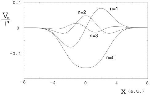
FIG. 1.:

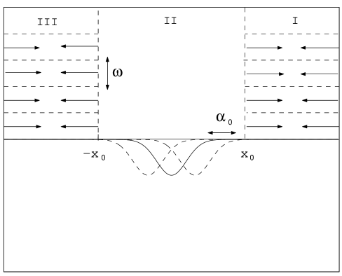
FIG. 2.:

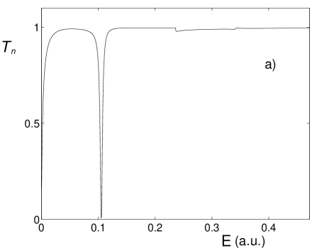
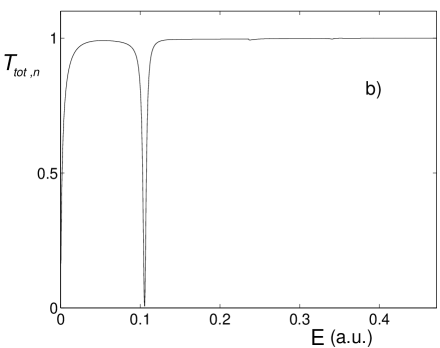
FIG. 3.:

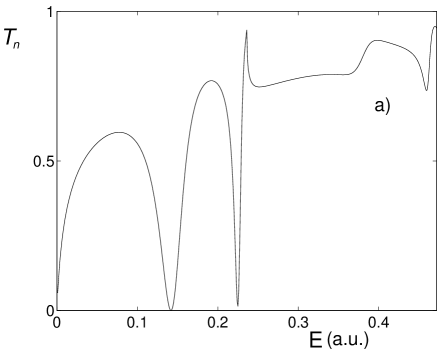
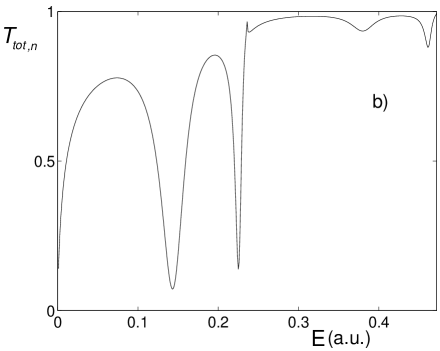
FIG. 4.:

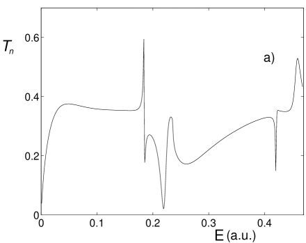
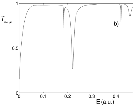
FIG. 5.:

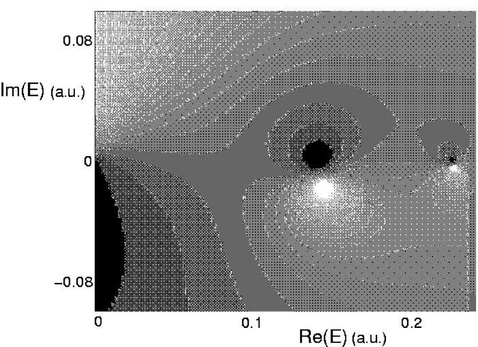
FIG. 6.:

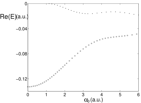
FIG. 7.:

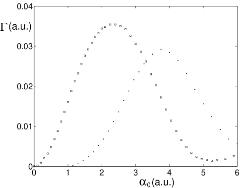
FIG. 8.:

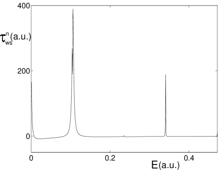
FIG. 9.:

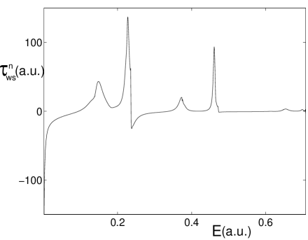
FIG. 10.:

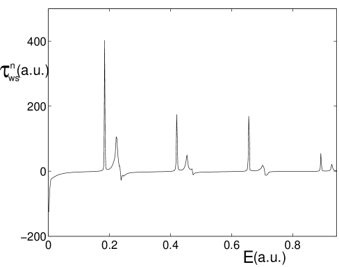
FIG. 11.:

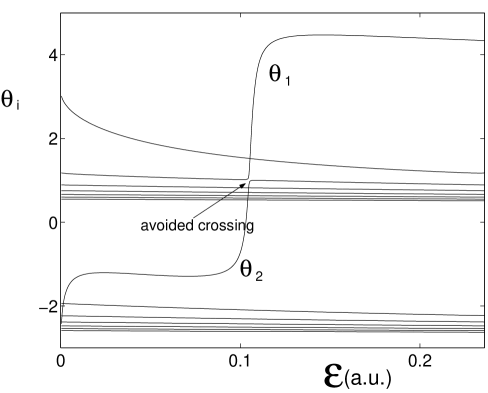
FIG. 12.:

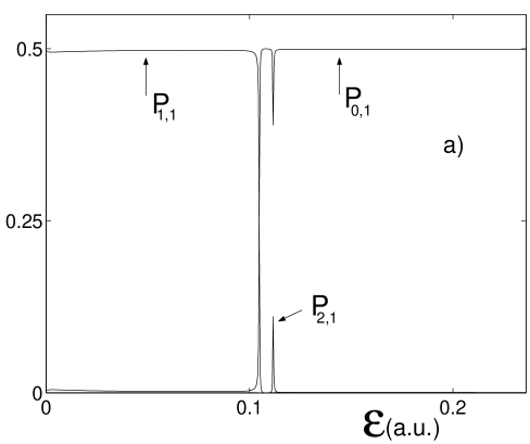
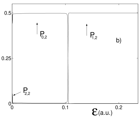
FIG. 13.:

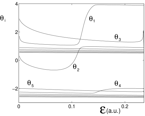
FIG. 14.:

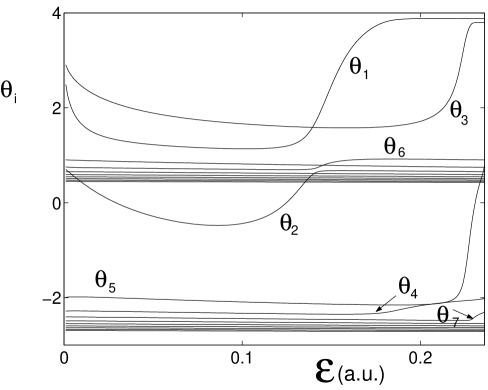
FIG. 15.:

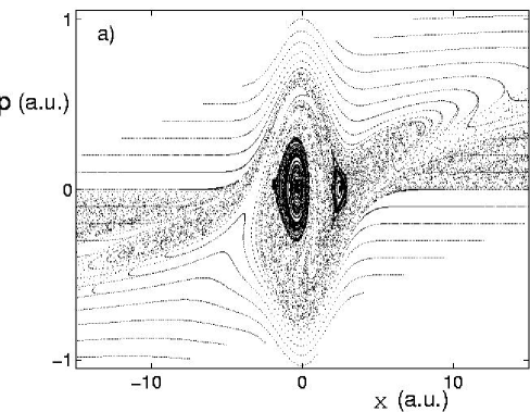
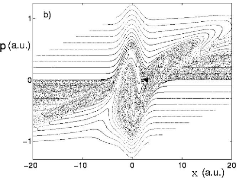
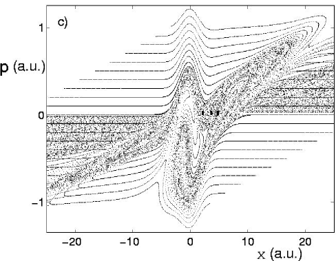
FIG. 16.:

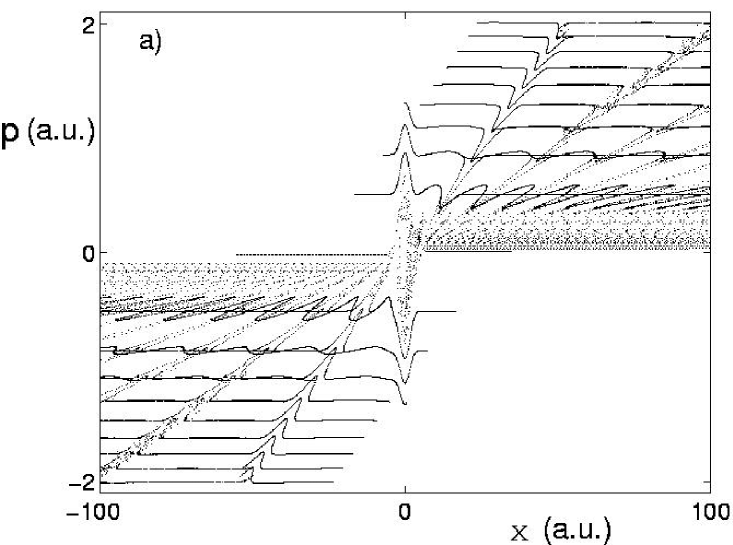
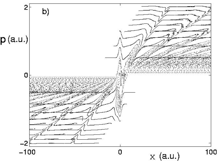
FIG. 17.:

REFERENCES

- [1] M. Gavrila and J. Z. Kaminski, Phys. Rev. Lett. 52, 613 (1984)
- [2] M. Pont, N. R. Walet, M. Gavrila, and C. W. McCurdy, Phys. Rev. Lett. 61, 939 (1988); M. Pont and M. Gavrila, Phys. Rev. Lett. 65, 2362 (1990)
- [3] K. Burnett, P. L. Knight, B. R. M. Piraux, and V. C. Reed, Phys. Rev. Lett 66, 301 (1991); K. C. Kulander, K. J. Schafer, and J. L. Krause, Phys. Rev. Lett. 66, 2601 (1991); Q. Su, J. H. Eberly, and J. Javanainen, Phys. Rev. Lett. 64, 862 (1990)
- [4] M. P. de Boer, J. H. Hoogenraad, R. B. Vrijen, R. C. Constantinescu, L. D. Noordam, and H. G. Muller, Phys. Rev. A 50, 4085 (1994); N. J. van Druten, R. C. Constantinescu, J. M. Schins, H. Nieuwenhuize and H. G. Muller, Phys. Rev. A 55, 622 (1997)
- [5] C. O. Reinhold, J. Burgdörfer, M. T. Frey, and F. B. Dunning, Phys. Rev. Lett. 79, 5226 (1997)
- [6] H. A. Kramers, Collected Scientific Papers (North-Holland, Amsterdam, 1956), p.272.
- [7] W. C. Henneberger, Phys. Rev. Lett. 21, 838 (1968).
- [8] L. Dimou and F. H. M. Faisal, Phys. Rev. Lett. 59, 872 (1987); L. A. Collins and G. Csanak, Phys. Rev. A 44, R5343 (1991)
- [9] R. Bhatt, B. Piraux, and K. Burnett, Phys. Rev. A 37, 98 (1988)
- [10] J. N. Bardsley and M. J. Comella, Phys. Rev. A 39, 2252 (1989)
- [11] G. Yao and S.-I Chu, Phys. Rev. A 45, 6735 (1992)
- [12] M. Marinescu and M. Gavrila, Phys. Rev. A 53, 2513 (1996)
- [13] T. Timberlake and L. E. Reichl, to appear in Phys. Rev. A, vol.64
- [14] W. Li and L. E. Reichl, Phys. Rev. B 60, 15732 (1999)
- [15] J. H. Shirley, Phys. Rev. 138, B979 (1965)
- [16] A. S. Fearnside, R. M. Portvliege, and R. Shakeshaft, Phys. Rev. A 51, 1471 (1995)
- [17] U. Fano, Phys. Rev. 124, 1866 (1961)
- [18] E. Tekman and P. F. Bagwell, Phys. Rev. B 48, 2553 (1993)
- [19] W. Porod, Zhi-an Shao, and C. S. Lent, Phys. Rev. B 48, 8495 (1993)
- [20] E. P. Wigner, Phys. Rev. 98, 145 (1955)
- [21] F. T. Smith, Phys. Rev. 118, 349 (1960)
- [22] K. Na and L. E. Reichl, Phys. Rev. B 59, 13073 (1999)
- [23] T. Timberlake and L. E. Reichl, Phys. Rev. A 59, 2886 (1999)
- [24] M. Henseler, T. Dittrich, and K. Richter (submitted to Phys. Rev. E)
- [25] Methods in Computational Physics edited by B. Alder et. al. (Academic Press New York and London 1966), p.16