Alternative interpretation of the sign reversal of secondary Bjerknes force acting between two pulsating gas bubbles

Abstract

It is known that in a certain case, the secondary Bjerknes force, which is a radiation force acting between pulsating bubbles, changes, e.g., from attraction to repulsion as the bubbles approach each other. In this paper, a theoretical discussion of this phenomenon for two spherical bubbles is described. The present theory based on analysis of the transition frequencies of interacting bubbles [M. Ida, Phys. Lett. A 297, 210 (2002)] provides an interpretation, different from previous ones (e.g., by Doinikov and Zavtrak [Phys. Fluids 7, 1923 (1995)]), of the phenomenon. It is shown, for example, that the reversal that occurs when one bubble is smaller and another is larger than a resonance size is due to the second-highest transition frequency of the smaller bubble, which cannot be obtained using traditional natural-frequency analysis.

I INTRODUCTION

It is known that two gas bubbles pulsating in an acoustic field undergo an interaction force called the secondary Bjerknes force ref1 ; ref2 ; ref3 . This force is attractive when the bubbles pulsate in-phase with each other, while it is repulsive otherwise; that is, the phase property of the bubbles plays an important role in determining the sign of the force. In a seminal paper published in 1984 ref4 , Zabolotskaya, using a linear coupled oscillator model, showed theoretically that in a certain case, the sign of the force may change as the bubbles come closer to one another. This theoretical prediction was ensured by recent experiments that captured the stable, periodic translational motion of two coupled bubbles ref12 , resulting from the sign reversal of the force at a certain distance between the bubbles. Zabolotskaya assumed that this sign reversal is due to variation in the natural frequencies of the interacting bubbles, which results in shifts of their pulsation phases. The theoretical formula Zabolotskaya derived to evaluate the natural frequencies of two interacting bubbles, which corresponds to one given previously by Shima ref5 , is represented as

$$(\omega_{10}^{2}-\omega^{2})(\omega_{20}^{2}-\omega^{2})-\frac{R_{10}R_{20}}{D^{2}}\omega^{4}\approx 0,$$ (1)

where $R_{10}$ and $R_{20}$ are the equilibrium radii of the bubbles, $\omega_{10}$ and $\omega_{20}$ are their partial natural (angular) frequencies, $\omega$ is the angular frequency of an external sound, and $D$ is the distance between the centers of the bubbles. This equation predicts the existence of two natural frequencies per bubble, and is symmetric; namely, it exchanges 10 and 20 in the subscripts of the variables to reproduce the same equation, meaning that the two bubbles have the same natural frequencies.

During the last decade, a number of studies regarding the sign reversal of the force have been performed ref6 ; ref7 ; ref8 ; ref9 ; ref10 ; ref11 ; ref12 ; ref13 ; ref20 . Among them, Refs. ref8 ; ref9 ; ref13 also considered the relevance of the change in the natural frequencies (or resonance frequencies ref22 ) to the sign reversal. In the present paper, we focus our attention on this case, although it has been shown that other factors, such as the nonlinearity in bubble pulsation ref6 ; ref10 ; ref11 ; ref13 ; ref20 and the higher-order terms appearing in the time-averaged interaction force ref12 which has been neglected in previous works, can also cause the sign reversal.

In 1995, Doinikov and Zavtrak ref8 , using a linear mathematical model in which the multiple scattering of sound between bubbles is taken into account more rigorously, predicted again the sign reversal. They also asserted that this reversal is due to the change in the natural frequencies. They assumed that the natural frequencies of both bubbles increase as the bubbles approach each other, resulting sometimes in the sign reversal. When, for example, both bubbles are larger than the resonance size (i.e., the case of $\omega_{10}<\omega$ and $\omega_{20}<\omega$) and the distance between them is large enough, they pulsate in-phase with each other. As the bubbles approach each other, the natural frequency of a smaller bubble may first, at a certain distance, rise above the driving frequency, and in turn the bubbles’ pulsations become antiphase; the force then changes from attractive to repulsive. When, on the other hand, one bubble is larger and the other is smaller than the resonance size (e.g., $\omega_{10}>\omega>\omega_{20}$) and the distance between them is large, they pulsate out-of-phase with each other and the force is repulsive. As the distance between the bubbles becomes smaller, the natural frequencies of both bubbles may rise, and when the natural frequency of a larger bubble rises above the driving frequency, the repulsive force may turn into attraction. This interpretation is supported even in more recent papers ref11 ; ref20 .

Although this interpretation seems to explain the sign reversal well, it is opposed to the prediction given by Eq. (1) which reveals that the higher natural frequency (converging to the partial natural frequency of a smaller bubble for $D\to\infty$ ref5 ; ref14 ) increases but the lower one (converging to the partial natural frequency of a larger bubble for $D\to\infty$) decreases as the bubbles approach each other.

In 2001, Harkin et al. ref13 performed an extensive theoretical study concerning the translational motion of two acoustically coupled gas bubbles in a weak and a moderate driving sound field. Their theoretical model derived from first principles supports the experimental results by Barbat et al. ref12 . In Sec. 7 of that paper, Harkin et al. also considered the influence of the change in natural frequencies on the sign of the force in order to explain the sign reversal for $\omega_{10}<\omega$ and $\omega_{20}<\omega$. Their explanation based on a formula given directly by Eq. (1) is essentially the same as those by Zabolotskaya ref4 and by Doinikov & Zavtrak ref8 ; ref9 .

The authors should note here that all the previous theoretical models mentioned above can describe (or explain) the sign reversal. However, the interpretation we will provide in the present paper is different from the previous ones.

The aim of this paper is to give an alternative interpretation of the sign reversal, one that may be more accurate than the previous ones that are based on the natural-frequency analysis. Recently, having reexamined the linear coupled oscillator model used frequently to analyze the dynamics of acoustically coupled bubbles (see Ref. ref14 and references therein), we found that a bubble interacting with a neighboring bubble has three “transition frequencies”, defined as the driving frequencies for which the phase difference between an external sound and the bubble’s pulsation becomes $\pi/{\it 2}$ (or ${\it 3}\pi/{\it 2}$), two of which correspond to the natural frequencies ref14 . Among the three transition frequencies, the lowest one decreases and the remaining two increase as the bubbles approach each other. Meanwhile, for $D\to\infty$ only one of them converges to the partial natural frequency of the corresponding bubble. Namely, the transition frequencies defined as above are asymmetric. The use of the transition frequencies would allow us an accurate understanding of the sign reversal, because observing these frequencies provides more detailed insights of the bubbles’ phase properties rather than that provided by the natural-frequency analysis. Using the theory for the transition frequencies, we arrive at a novel interpretation of the sign reversal.

II THEORIES

In this section, we briefly review the previously expounded theories regarding the natural frequencies, the transition frequencies, and the secondary Bjerknes force.

II.1 Natural frequencies and transition frequencies

Let us consider the linear volume oscillation of $N$–bubble system immersed in an incompressible liquid. Suppose that the time-dependent radius of bubble $j$, $R_{j}$, can be represented as $R_{j}=R_{j0}+e_{j}(t)$ and $\left|{e_{j}}\right|\ll R_{j0}$, where $R_{j0}$ and $e_{j}$ are the equilibrium radius and the deviation of the radius, respectively, and $j=1,2,\ldots,N$ . The radius deviation can be determined by solving the linear oscillator model (see, e.g., Ref. ref23 ),

$$\ddot{e}_{j}+\omega_{j0}^{2}e_{j}+\delta_{j}\dot{e}_{j}=-\frac{{p_{{\rm d},j}}}{{\rho R_{j0}}},$$ (2)

where

$$\omega_{j0}=\sqrt{\frac{{3\kappa_{j}P_{0}+(3\kappa_{j}-1)2\sigma/R_{j0}}}{{\rho R_{j0}^{2}}}}$$

are the partial natural (angular) frequencies of bubble $j$, $\delta_{j}$ is the damping coefficient determined based on the damping characteristics of the bubbles ref15 , $p_{{\rm d},j}$ is the driving pressure acting on bubble $j$, $\kappa_{j}$ is the effective polytropic exponent of the gas inside the bubbles, $P_{0}$ is the static pressure, $\sigma$ is the surface tension, $\rho$ is the density of the liquid surrounding the bubbles, and the overdots denote the time derivation. The driving pressure is represented by the sum of $p_{{\rm ex}}$ and the sound pressure scattered by the surrounding bubbles, $p_{\rm s}$, as

$$p_{{\rm d},j}=p_{{\rm ex}}+\sum\limits_{k=1,k\neq j}^{N}{p_{{\rm s},j\,k}}.$$

The value of $p_{{\rm s},j\,k}$ is determined by integrating the momentum equation for linear sound waves, $\partial p/\partial r=-\rho\partial u/\partial t$, coupled with the divergence-free condition, $\partial(r^{2}u)/\partial r=0$, where $r$ is the radial coordinate measured from the center of a bubble and $u$ is the velocity along $r$. Resultantly, the driving pressure is determined as

$$p_{{\rm d},j}=p_{{\rm ex}}+\rho\sum\limits_{k=1,k\neq j}^{N}{\frac{{R_{k0}^{2}}}{{D_{j\,k}}}\ddot{e}_{k}},$$ (3)

where $D_{j\,k}$ is the distance between the centers of bubbles $j$ and $k$.

In a single-bubble case (i.e., for $N=1$), Eq. (2) is reduced to

$$\ddot{e}_{1}+\omega_{10}^{2}e_{1}+\delta_{1}\dot{e}_{1}=-\frac{{p_{{\rm ex}}}}{{\rho R_{10}}}.$$ (4)

Assuming that $p_{{\rm ex}}$ is written in the form of $p_{{\rm ex}}=-P_{a}\sin\omega t$ ($P_{a}$ is a positive constant), the harmonic steady-state solution of Eq. (4) is given by

$$e_{1}=K_{S1}\sin(\omega t-\phi_{S1}),$$

with

$$K_{S1}=\frac{{P_{a}}}{{\rho_{0}R_{10}}}\sqrt{\frac{1}{{(\omega_{10}^{2}-\omega^{2})^{2}+\delta_{1}^{2}\omega^{2}}}},$$

$$\phi_{S1}=\tan^{-1}\left({\frac{{\delta_{1}\omega}}{{\omega_{10}^{2}-\omega^{2}}}}\right).$$

From this result, one knows that the phase difference of $\phi_{S1}=\pi/2$ appears (or, roughly speaking, the phase reversal takes place) only at the natural frequency $\omega_{10}$ ref24 , and the resonance response occurs at (or, more correctly, near) the same driving frequency.

For $N=2$, Eq. (2) is reduced to

$$\ddot{e}_{1}+\omega_{10}^{2}e_{1}+\delta_{1}\dot{e}_{1}=-\frac{{p_{{\rm ex}}}}{{\rho R_{10}}}-\frac{{R_{20}^{2}}}{{R_{10}D}}\ddot{e}_{2},$$ (5)

$$\ddot{e}_{2}+\omega_{20}^{2}e_{2}+\delta_{2}\dot{e}_{2}=-\frac{{p_{{\rm ex}}}}{{\rho R_{20}}}-\frac{{R_{10}^{2}}}{{R_{20}D}}\ddot{e}_{1},$$ (6)

where $D=D_{12}=D_{21}$. It is known that for a weak forcing (i.e., $P_{a}\ll P_{0}$), this system has third-order accuracy with respect to $1/D$, although it has terms of up to first order (the last terms) ref13 . The harmonic steady-state solution for $e_{1}$ is

$$e_{1}=K_{1}\sin(\omega t-\phi_{1}),$$

where

$$K_{1}=\frac{{P_{a}}}{{R_{10}\rho}}\sqrt{A_{1}^{2}+B_{1}^{2}},$$

$$\phi_{1}=\tan^{-1}\left({\frac{{B_{1}}}{{A_{1}}}}\right)\in[0,2\pi],$$

with

$$A_{1}=\frac{{H_{1}F+M_{2}G}}{{F^{2}+G^{2}}},\quad B_{1}=\frac{{H_{1}G-M_{2}F}}{{F^{2}+G^{2}}},$$

$$F=L_{1}L_{2}-\frac{{R_{10}R_{20}}}{{D^{2}}}\omega^{4}-M_{1}M_{2},$$

$$G=L_{1}M_{2}+L_{2}M_{1},\quad H_{1}=L_{2}+\frac{{R_{20}}}{D}\omega^{2},$$

$$L_{1}=\omega_{10}^{2}-\omega^{2},\quad L_{2}=\omega_{20}^{2}-\omega^{2},$$

$$M_{1}=\delta_{1}\omega,\quad M_{2}=\delta_{2}\omega.$$

Exchanging 1 and 2 (or 10 and 20) in the subscripts of these equations yields the expressions for bubble 2.

The formula for the natural frequency, Eq. (1), is derived so that $K_{1}\to\infty$ for $\delta_{1}\to 0$ and $\delta_{2}\to 0$. Namely,

$$F=L_{1}L_{2}-\frac{{R_{10}R_{20}}}{{D^{2}}}\omega^{4}=0.$$

As mentioned already, this equation predicts the existence of up to two natural frequencies in a double-bubble system.

The transition frequencies of bubble 1 are determined so that $\phi_{1}$ becomes $\pi/2$ (or $3\pi/2$). Because $F^{2}+G^{2}\neq 0$ ref14 , the resulting formula for deriving the transition frequencies of bubble 1 is

$$H_{1}F+M_{2}G=0.$$ (7)

Assuming $\delta_{1}\to 0$ and $\delta_{2}\to 0$ reduces this to

$$H_{1}F=\left({L_{2}+\frac{{R_{20}}}{D}\omega^{2}}\right)\left({L_{1}L_{2}-\frac{{R_{10}R_{20}}}{{D^{2}}}\omega^{4}}\right)=0.$$ (8)

As was proven in Ref. ref14 , this equation predicts the existence of up to three transition frequencies per bubble. Furthermore, as pointed out in the same article, the terms in the second $\left(\cdots\right)$ of Eq. (8) are the same as those on the left-hand side of Eq. (1). These results mean that in a double-bubble case the phase reversal of a bubble’s pulsation can take place not only at its natural frequencies but also at one other frequency. Because $H_{1}\neq H_{2}$, Eq. (8) (and also Eq. (7)) is asymmetric, meaning that the bubbles have different transition frequencies.

A preliminary discussion for a $N$–bubble system ref19 showed that a bubble in the system has up to $2N-1$ transition frequencies, $N$ ones of which correspond to the natural frequency. Namely, a bubble has an odd number of transition frequencies. This result can be understood as follows: Even in a multibubble case, a bubble’s pulsation may be in-phase or out-of-phase with a driving sound ref25 when the driving frequency is much lower or much higher, respectively, than its natural frequencies; thus, in order to interpolate these two extremes consistently an odd number of phase reversals are necessary ref19 .

II.2 Secondary Bjerknes force

The secondary Bjerknes force acting between the bubbles for sufficiently weak forcing is expressed with ref1 ; ref2 ; ref3 ; ref4 ; ref12 ; ref13

$${\bf F}\propto\left\langle{\dot{V}_{1}\dot{V}_{2}}\right\rangle\frac{{{\bf r}_{2}-{\bf r}_{1}}}{{\left\|{{\bf r}_{2}-{\bf r}_{1}}\right\|^{3}}}\propto K_{1}K_{2}\cos(\phi_{1}-\phi_{2})\frac{{{\bf r}_{2}-{\bf r}_{1}}}{{\left\|{{\bf r}_{2}-{\bf r}_{1}}\right\|^{3}}},$$ (9)

where $V_{j}$ and ${\bf r}_{j}$ are the volume and the position, respectively, of bubble $j$, $\left\langle\cdots\right\rangle$ denotes the time average, and $\left\|{{\bf r}_{2}-{\bf r}_{1}}\right\|=D$. The sign reversal of this force occurs only when the sign of $\cos(\phi_{1}-\phi_{2})$ (or of $\left\langle{\dot{V}_{1}\dot{V}_{2}}\right\rangle$) changes, because $K_{1}>0$ and $K_{2}>0$. If the phase shifts resulting from the radiative interaction between bubbles are neglected, this force is repulsive when $\omega$ stays between $\omega_{10}$ and $\omega_{20}$, and is attractive otherwise ref1 . In the case where the radiative interaction is taken into consideration, the frequency within which the force is repulsive shifts toward a higher range, see, e.g., Refs. ref8 ; ref9 .

The formulae reviewed above, except for that regarding the transition frequencies (Eqs. (7) and (8)), are classical, and almost the same ones have previously been used in Ref. ref4 . As will be shown in the next section, however, the following investigation based on Eq. (7) coupled with Eq. (9) gives a different interpretation of the sign reversal from the previous ones described using only the natural frequencies.

III RESULTS AND DISCUSSION

In this section, we investigate the relationship between the transition frequencies and the sign of the secondary Bjerknes force by using some examples. The first example is the case of $R_{10}=2$ mm and $R_{20}=5$ mm, which corresponds to a case used in Ref. ref9 . We assume that the bubbles are filled with a gas having a specific heat ratio of $\gamma=1.4$, and the surrounding material is water ($\sigma=0.0728$ N/m, $\rho=1000$ kg/m³, $P_{0}=1$ atm, and the speed of sound $c=1500$ m/s). For the damping coefficient, we adopt that used for radiation and thermal losses:

$$\delta_{j}=\frac{{\omega^{2}R_{j0}}}{c}+\beta_{{\rm th},j},$$ (10)

where the thermal damping coefficient $\beta_{{\rm th},j}$ and the effective polytropic exponent $\kappa_{j}$ are determined by ref21 ; ref15 ; ref8

$$\beta_{{\rm th},j}=\frac{{\omega_{j0}^{2}}}{\omega}d_{{\rm th},j},$$

$$\kappa_{j}=\gamma\left[{\left({1+d_{{\rm th},j}^{2}}\right)\left({1+\frac{{3(\gamma-1)(\sinh X-\sin X)}}{{X(\cosh X-\cos X)}}}\right)}\right]^{-1},$$

with

$$d_{{\rm th},j}=3(\gamma-1)$$

$$\times\frac{{X(\sinh X+\sin X)-2(\cosh X-\cos X)}}{{X^{2}(\cosh X-\cos X)+3(\gamma-1)X(\sinh X-\sin X)}},$$

$$X=R_{j0}(2\omega/\chi_{G})^{1/2},$$

where we set $\chi_{G}=2\times 10^{-5}$ m² s^-1.

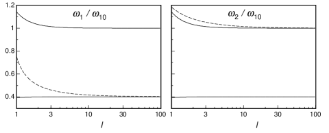
Figure 1: Transition frequencies $\omega_{1}$ (rad/s) and $\omega_{2}$ (rad/s) for $R_{10}=2$ mm, $R_{20}=5$ mm, and the reduced damping, normalized by $\omega_{10}$ (rad/s). The dashed lines show the transition frequencies that do not cause the resonance.

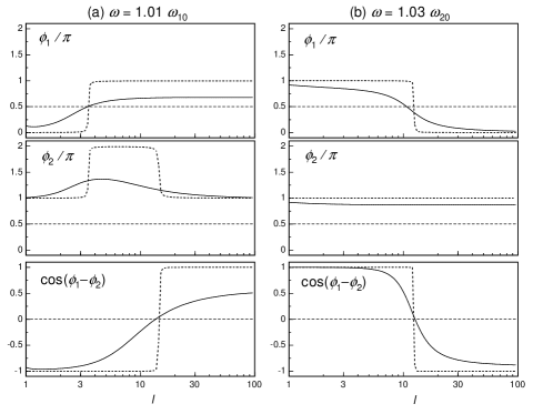
Figure 2: $\phi_{1}/\pi$, $\phi_{2}/\pi$, and $\cos(\phi_{1}-\phi_{2})$ for (a) $\omega=1.01\omega_{10}$ (rad/s) and (b) $\omega=1.03\omega_{20}$ (rad/s), as functions of $l$. The dashed curves and the solid lines show the results given using the reduced damping and the real damping, respectively.

In order to clarify the following discussion, we first present results for the idealized condition of $\delta_{j}\approx 0$ by resetting $\delta_{j}\to\delta_{j}/100$, and subsequently provide results given by the direct use of Eq. (10). Figure 1 shows the transition frequencies of the bubbles, $\omega_{1}$ and $\omega_{2}$, calculated using Eq. (7) with the reduced damping, normalized by $\omega_{10}$ ($=\omega_{1}$ for $D\to\infty$). In those figures, $l$ denotes the normalized distance defined as $l=D/(R_{10}+R_{20})$. As mentioned previously, we can observe three transition frequencies, only one of which converges to $\omega_{j0}$ of the corresponding bubble for $l\to\infty$. The second-highest transition frequency of bubble 2 is almost equal to the highest one of bubble 1; thus, the highest one of bubble 2 is higher than that of bubble 1. The second highest one of bubble 1 and the highest one of bubble 2 do not cause the resonance response ref14 .

The dashed curves displayed in Fig. 2(a) show $\phi_{1}$, $\phi_{2}$, and $\cos(\phi_{1}-\phi_{2})$, respectively, as functions of $l$. Here the driving frequency is assumed to be $\omega=1.01\omega_{10}$, i.e., slightly above $\omega_{10}$. (In the present study, the driving frequency is set as $\omega\approx\omega_{10}$ or $\omega\approx\omega_{20}$ so that the sign reversal takes place at a sufficiently large $l$ where the accuracy of Eqs. (5) and (6) is guaranteed.) As mentioned in Sec. I, it is known already that the sign reversal can take place when $\omega>\omega_{10}>\omega_{20}$ or $\omega_{10}>\omega>\omega_{20}$; the present setting corresponds to the former case. We can observe one and two sharp shifts of $\phi_{1}$ and $\phi_{2}$, respectively. At $l\approx 3$, both $\phi_{1}$ and $\phi_{2}$ shift almost simultaneously, but the sign reversal does not occur because the phase difference $\phi_{1}-\phi_{2}$ is hardly changed. At $l\approx 13$, only $\phi_{2}$ shifts, resulting in the sign reversal. In the former case, the phase shifts are caused by the natural frequencies. As mentioned previously, when $\delta_{j}\approx 0$ both the bubbles have (almost) the same natural frequencies. The simultaneous phase shift, thus, appears. The change of $\phi_{2}$ in the later case is apparently due to the highest transition frequency of bubble 2, which cannot be obtained by the traditional natural-frequency analysis. Namely, this sign reversal cannot be interpreted by using only the natural frequencies.

We should note here that, to compute the phase delays $\phi_{1}$ and $\phi_{2}$, we used the “${\rm atan2}(a,b)$” function in the C language, which returns $\tan^{-1}(b/a)\in[-\pi,\pi]$, and, furthermore, adopted the operation

$$\phi_{j}=\left\{{\begin{array}[]{*{20}c}{{\rm atan2}(A_{j},B_{j})+2\pi\hfill}&{{\rm if}\,\,\,{\rm atan2}(A_{j},B_{j})<0,\hfill}\\ {{\rm atan2}(A_{j},B_{j})\hfill}&{{\rm otherwise\hfill}}\\ \end{array}}\right.$$

in order to obtain results for $l\gg 1$ that are consistent with the established knowledge of single-bubble dynamics, e.g., $\phi_{j}\approx\pi$ when $\omega>\omega_{j0}$ and $\delta_{j}\approx 0$ ($j=1$ or $2$).

The dashed curves displayed in Fig. 2(b) show results for $\omega=1.03\omega_{20}$ ($=0.413\omega_{10}$), i.e., for $\omega_{10}>\omega>\omega_{20}$. In this case, we can observe only one sharp shift of $\phi_{1}$ at $l\approx 12$, causing the sign reversal. This shift of $\phi_{1}$ is due to the second-highest transition frequency of bubble 1 (this frequency also not corresponding to the natural frequency!), because the lowest transition frequencies of both the bubbles decrease as $l$ decreases.

These results reveal that in the above cases, the transition frequencies other than the natural frequencies cause the sign reversal of the secondary Bjerknes force. This conclusion is obviously different from the previous interpretations described by means of the natural frequencies ref4 ; ref8 ; ref9 ; ref13 .

It is interesting to point out that, in the case where $\omega>\omega_{10}>\omega_{20}$ and $\omega\approx\omega_{10}$, the phase delay of the larger bubble was sometimes greater than $\pi$ (see Fig. 2(a)). Such a result cannot be given by a single-bubble model which predicts a phase delay of up to $\pi$. This may be explained as follows: When $\omega>\omega_{10}>\omega_{20}$ is true and $l$ is sufficiently large, both bubbles pulsate out-of-phase with $p_{{\rm ex}}$, emitting sound waves whose phases are also out-of-phase with $p_{{\rm ex}}$. As $l$ decreases, if $\omega\approx\omega_{10}$, the amplitude of the sound wave emitted by bubble 1 measured at ${\bf r}_{2}$ can be greater than the amplitude of $p_{{\rm ex}}$. In this situation, bubble 2 is driven by a sound wave whose oscillation phase is delayed by almost $\pi$ from that of $p_{{\rm ex}}$. This results in $\phi_{2}>\pi$, because the pulsation phase of bubble 2 delays further from that of the sound wave.

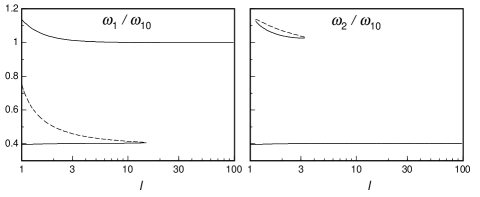
Figure 3: Same as in Fig. 1, but for the real damping.

We show the here results given by using Eq. (10) in order to examine the influences of the damping effects on the sign reversal and phase shifts. Figure 3 shows the recalculated transition frequencies. As already discussed ref14 , when the damping effects are not negligible, the bubbles have only one transition frequency in the large-$l$ region. The solid curves displayed in Fig. 2 show $\phi_{1}$, $\phi_{2}$, and $\cos(\phi_{1}-\phi_{2})$ for $\omega=1.01\omega_{10}$ and $\omega=1.03\omega_{20}$. Their tendencies are similar to those given with the reduced damping, although their profiles are smoothed significantly (Such a smoothing of the phase change by the damping effects is well known for a single-bubble case) and the points at which the sign reversal takes place are shifted slightly; the positions of these points are, in the case of $\omega=1.01\omega_{10}$, $l\approx 13.59$ for $\delta_{j}$ and $l\approx 14.57$ for $\delta_{j}/100$, and, in the case of $\omega=1.03\omega_{20}$, $l\approx 12.66$ for $\delta_{j}$ and $l\approx 12.48$ for $\delta_{j}/100$. Moreover, $\phi_{2}$ for $\omega=1.01\omega_{10}$ does not exceed $3\pi/2$ (the minimum value of $\omega_{2}$ larger than $\omega_{10}$ is ${\rm 1}{\rm.027}\omega_{10}$.); even so, the sign reversal occurs at almost the same point as that given with $\delta_{j}/100$, away from the point where $\phi_{1}=\pi/2$. This result may be interpreted as the “vestige” of the highest transition frequency of the larger bubble having given rise to this sign reversal. Detailed theoretical discussions for the slight shift in $l$ for $\cos(\phi_{1}-\phi_{2})=0$ due to the damping effects will be provided in a future paper.

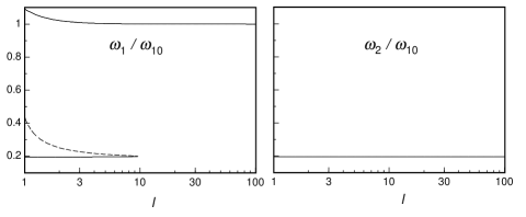
Figure 4: Transition frequencies $\omega_{1}$ (rad/s) and $\omega_{2}$ (rad/s) for $R_{10}=1$ $\mu$m, $R_{20}=4$ $\mu$m, and the real damping, normalized by $\omega_{10}$ (rad/s).

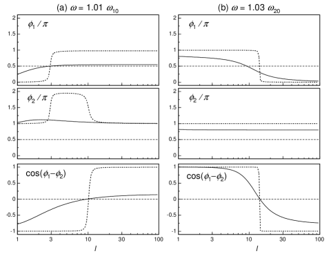
Figure 5: $\phi_{1}/\pi$, $\phi_{2}/\pi$, and $\cos(\phi_{1}-\phi_{2})$ for (a) $\omega=1.01\omega_{10}$ (rad/s) and (b) $\omega=1.03\omega_{20}$ (rad/s). The dashed curves denote the results for the reduced damping.

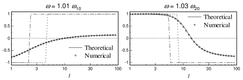
Figure 6: Comparison between the theoretical and the numerical results. The lines and the circles denote the theoretical and the numerical results, respectively, of $\cos(\phi_{1}-\phi_{2})$ for $\omega=1.01\omega_{10}$ (rad/s) and $1.03\omega_{20}$ (rad/s). Additionally, ${\mathop{\rm sgn}}\left(\left\langle{\dot{V}_{1}\dot{V}_{2}}\right\rangle\right)$ for $P_{a}/P_{0}=0.2$ (the dots) and $0.5$ (the dash-dotted curves) are plotted for a brief investigation of nonlinear effects.

Next, we show results for smaller bubbles ($R_{10}=1$ $\mu$m and $R_{20}=4$ $\mu$m). The value for viscous loss is used for the damping coefficients, i.e.,

$$\delta_{j}=\frac{{4\mu}}{{\rho R_{j0}^{2}}},$$ (11)

where the viscosity of water $\mu=1.002\times 10^{-3}$ kg/(m s). Because the thermal effect is neglected, $\kappa=\gamma=1.4$. Figure 4 shows the transition frequencies, and Figure 5 shows $\phi_{1}$, $\phi_{2}$, and $\cos(\phi_{1}-\phi_{2})$ for $\omega=1.01\omega_{10}$ and $\omega=1.03\omega_{20}$ ($=0.201\omega_{10}$) with $\delta_{j}/100$ (the dashed curves) and $\delta_{j}$ (the solid curves). The qualitative natures of these results are quite similar with the previous ones; thus, additional discussion may not be necessary. Using this example, we perform here a comparative study of the theoretical results with the numerical results in order to confirm the former’s correctness. In the numerical experiment, we employ the coupled RPNNP (Rayleigh, Plesset, Noltingk, Neppiras, and Poritsky) equations (see, e.g., Ref. ref14 );

$$R_{1}\ddot{R}_{1}+\frac{3}{2}\dot{R}_{1}^{2}-\frac{1}{\rho}p_{w,1}=-\frac{1}{\rho}\left[{p_{{\rm ex}}+\frac{\rho}{D}\frac{d}{{dt}}(R_{2}^{2}\dot{R}_{2})}\right],$$

$$R_{2}\ddot{R}_{2}+\frac{3}{2}\dot{R}_{2}^{2}-\frac{1}{\rho}p_{w,2}=-\frac{1}{\rho}\left[{p_{{\rm ex}}+\frac{\rho}{D}\frac{d}{{dt}}(R_{1}^{2}\dot{R}_{1})}\right],$$

where

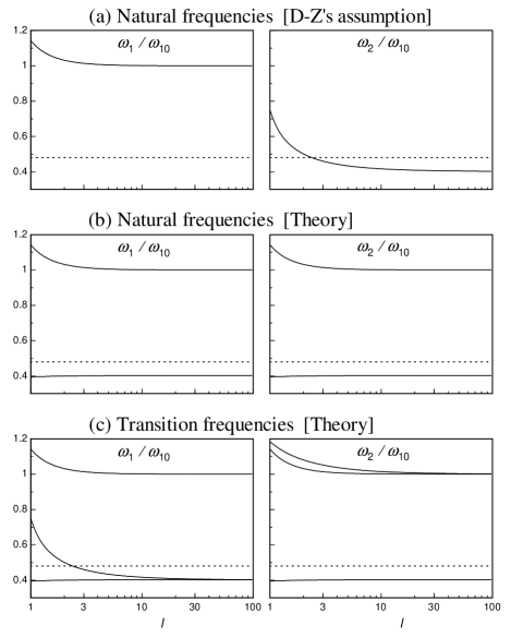
Figure 7: Characteristic frequencies of two coupled bubbles and different interpretations of the sign reversal. The dashed lines show a typical driving frequency lying between $\omega_{10}$ and $\omega_{20}$, where $\omega_{10}>\omega_{20}$ is assumed. Doinikov and Zavtrak assumed that the natural frequencies of both the bubbles increase as the bubbles approach each other (a). Assuming this, the sign reversal for $\omega_{10}>\omega>\omega_{20}$ seems to be explained. This assumption is, however, inconsistent with the classical theory for natural frequencies (b). The present theory can explain this reversal without such an inconsistency (c).

$$p_{w,j}=\left({P_{0}+\frac{{2\sigma}}{{R_{j0}}}}\right)\left({\frac{{R_{j0}}}{{R_{j}}}}\right)^{3\kappa}-\frac{{2\sigma}}{{R_{j}}}-\frac{{4\mu\dot{R}_{j}}}{{R_{j}}}-P_{0}.$$

This system of nonlinear differential equations are solved numerically through the use of the fourth-order Runge-Kutta method in which $R_{1}$, $R_{2}$, $\dot{R}_{1}$, and $\dot{R}_{2}$ are used as dependent variables, and $\left\langle{R_{1}^{2}\dot{R}_{1}R_{2}^{2}\dot{R}_{2}}\right\rangle$ [$\propto\left\langle{\dot{V}_{1}\dot{V}_{2}}\right\rangle$ in Eq. (9)] is then calculated. The time average is performed during a sufficiently large period after the transients have decayed. Normalizing $\left\langle{R_{1}^{2}\dot{R}_{1}R_{2}^{2}\dot{R}_{2}}\right\rangle$ by $R_{10}^{2}R_{20}^{2}\max(\left|{R_{1}(t)-R_{10}}\right|)\max(\left|{R_{2}(t)-R_{20}}\right|)\omega^{2}/2$ yields the numerical approximation of $\cos(\phi_{1}-\phi_{2})$, where $\max(\left|{R_{j}(t)-R_{j0}}\right|)$ indicates the pulsation amplitude of bubble $j$ given numerically. The amplitude of the external sound is set to $P_{a}=0.01P_{0}$. In Figure 6, the numerical and the theoretical results are displayed in piles. These results are in excellent agreement, confirming the correctness of the theoretical results given above. In the same figure, we have shown additionally ${\mathop{\rm sgn}}\left(\left\langle{\dot{V}_{1}\dot{V}_{2}}\right\rangle\right)$ for $P_{a}=0.2P_{0}$ (the dots) and $0.5P_{0}$ (the dash-dotted curves) in order to briefly investigate nonlinear effects on the sign reversal, where ${\mathop{\rm sgn}}(X)=1$ for $X>0$ and ${\mathop{\rm sgn}}(X)=-1$ otherwise. In plotting these results, we omitted the data in the case where $R_{1}(t)+R_{2}(t)>D$ was observed during the computation. As is clearly shown, increasing the driving pressure reduces the distance for which the sign reversal takes place. This result appears to be consistent with the well-known nonlinear phenomenon that a strong driving pressure decreases a bubble’s (effective) resonance frequency, see, e.g., Refs. ref2 ; ref3 . (Imagine that the transition frequencies shown, e.g., in Fig. 1 decrease but the driving frequency holds, which might shorten the distance for ${\bf F}=0$.) More detailed and concrete discussions on the nonlinear effects will be provided in a future paper.

To summarize our discussion, we compare the present interpretation with the previous ones. Figure 7(a) shows the dependency of natural frequencies on $l$ that Doinikov and Zavtrak assumed ref8 ; ref9 . Their assumption explains the sign reversal occurring when $\omega_{10}>\omega>\omega_{20}$, for example, as taking place around $l$ at which $\omega_{2}=\omega$ is true. Yet, as mentioned, their assumption is inconsistent with the theoretical results regarding natural frequencies given previously ref4 ; ref5 (see Fig. 7(b)). On the other hand, it is difficult to determine by only observing the natural frequencies that the sign reversal can take place for $\omega_{10}>\omega>\omega_{20}$, because the classical theory does not show that a kind of characteristic frequency exists in the frequency region between $\omega_{10}$ and $\omega_{20}$. The present theory explains the sign reversal in this case as taking place around $l$ at which $\omega_{1}=\omega$ is true (see Fig. 7(c), where we assume for simplicity that the damping effect is negligible), and is consistent with the theory for natural frequencies because the transition frequencies include the natural frequencies.

IV CONCLUSION

We have investigated the influences of change in the transition frequencies of gas bubbles, resulting from their radiative interaction, on the sign of the secondary Bjerknes force. The most important point suggested in this paper is that the transition frequencies that cannot be derived by the natural-frequency analysis cause the sign reversal in the cases of both $\omega>\omega_{10}>\omega_{20}$ and $\omega_{10}>\omega>\omega_{20}$. This interpretation has not been proposed previously. The present results also show that the theory given in Ref. ref14 for evaluating the transition frequencies of interacting bubbles is a reasonable tool for accurately understanding the mechanism of this reversal. In a paper currently in preparation ref16 , we will use the direct numerical simulation technique ref17 ; ref18 to verify the present theoretical results.

Lastly, we make further remarks regarding the results described in Ref. ref9 . In that paper, the frequency of the external sound ($f=\omega/2\pi$) was assumed to be $f=63$ kHz, which is 60 times higher than the partial resonance frequency of a bubble of $R_{0}=3$ mm (1.094 kHz); nevertheless, the reversal was observed at a very small $l$. (In Ref. ref8 , the driving frequency is assumed to be comparable to the partial natural frequencies of bubbles, and the bubble radii are several tens of micrometers.) This result reveals implicitly that the mathematical model proposed in Ref. ref8 , which takes into account the shape deviation of the bubbles, predicts such a strong increase of the transition frequencies of closely coupled large bubbles that this increase cannot be explained by the classical model for coupled oscillators used here. Derivation of the transition frequencies of Doinikov and Zavtrak’s model would be an interesting subject for future study.

- (1) L. A. Crum, J. Acoust. Soc. Am. 57, 1363 (1975).
- (2) A. Prosperetti, Ultrasonics 22, 115 (1984).
- (3) W. Lauterborn, T. Kurz, R. Mettin, and C. D. Ohl, Adv. Chem. Phys. 110, 295 (1999).
- (4) E. A. Zabolotskaya, Sov. Phys. Acoust. 30, 365 (1984).
- (5) T. Barbat, N. Ashgriz, and C.-S. Liu, J. Fluid Mech. 389, 137 (1999).
- (6) A. Shima, Trans. ASME, J. Basic Eng. 93, 426 (1971).
- (7) H. Oguz and A. Prosperetti, J. Fluid Mech. 218, 143 (1990).
- (8) N. A. Pelekasis and J. A. Tsamopoulos, J. Fluid Mech. 254, 501 (1993).
- (9) A. A. Doinikov and S. T. Zavtrak, Phys. Fluids 7, 1923 (1995).
- (10) A. A. Doinikov and S. T. Zavtrak, J. Acoust. Soc. Am. 99, 3849 (1996).
- (11) R. Mettin, I. Akhatov, U. Parlitz, C. D. Ohl, and W. Lauterborn, Phys. Rev. E 56, 2924 (1997).
- (12) A. A. Doinikov, Phys. Rev. E 59, 3016 (1999).
- (13) A. Harkin, T. J. Kaper, and A. Nadim, J. Fluid Mech. 445, 377 (2001).
- (14) A. A. Doinikov, Phys. Rev. E 64, 026301 (2001).
- (15) Strictly speaking, the natural frequency is different from the resonance frequency. Because these frequencies are almost equal to each other in many cases, however, we treat them as the same, as has been done frequently.
- (16) M. Ida, Phys. Lett. A 297, 210 (2002).
- (17) C. Feuillade, J. Acoust. Soc. Am. 98, 1178 (1995).
- (18) A. Prosperetti, Ultrasonics 22, 69 (1984).
- (19) This is not true when the driving pressure is strong. See, e.g., I. Akhatov, R. Mettin, C. D. Ohl, U. Parlitz, and W. Lauterborn, Phys. Rev. E 55, 3747 (1997).
- (20) M. Ida, J. Phys. Soc. Japan 71, 1214 (2002).
- (21) In this case, “in-phase”, for example, means that during the sound pressure is positive, the bubble’s radius is smaller than its equilibrium size and hence the deviation of the bubble’s internal pressure is positive.
- (22) L. A. Crum and A. I. Eller, J. Acoust. Soc. Am. 48, 181 (1969).
- (23) M. Ida, e-print, physics/0111138 (still in preparation).
- (24) M. Ida, Comput. Phys. Commun. 150, 300 (2003).
- (25) M. Ida, Comput. Phys. Commun. 132, 44 (2000).