Nonlinearities and Effects of Transverse Beam Size in Beam Position Monitors (revised)

Abstract

The fields produced by a long beam with a given transverse charge distribution in a homogeneous vacuum chamber are studied. Signals induced by a displaced finite-size beam on electrodes of a beam position monitor (BPM) are calculated and compared to those produced by a pencil beam. The non-linearities and corrections to BPM signals due to a finite transverse beam size are calculated for an arbitrary chamber cross section. Simple analytical expressions are given for a few particular transverse distributions of the beam current in a circular or rectangular chamber. Of particular interest is a general proof that in an arbitrary homogeneous chamber the beam-size corrections vanish for any axisymmetric beam current distribution.

I Introduction

In many accelerators, especially in ion linacs and storage rings, beams occupy a significant fraction of the vacuum chamber cross section. On the other hand, an analysis of beam-induced signals in beam position monitors (BPMs) is usually restricted to the case of an infinitely small beam cross section (pencil beam). In this paper we consider the problem for a vacuum chamber with an arbitrary but constant cross section, and calculate, for a given transverse charge distribution of an off-axis relativistic beam, the fields produced by the beam on the chamber wall. Comparing those with the fields of a pencil beam gives us corrections (e.g., to BPM signals) due to a finite transverse size of the beam.

Let a vacuum chamber have an arbitrary single-connected cross section $S$ that does not change as a beam moves along the chamber axis $z$, and perfectly conducting walls. We consider the case of $(\omega b/\beta\gamma c)^{2}\ll 1$, where $\omega$ is the frequency of interest, $\beta c$ is the beam velocity, $\gamma=1/\sqrt{1-\beta^{2}}$, and $b$ is a typical transverse dimension of the vacuum chamber. It includes both the ultra relativistic limit, $\gamma\gg 1$, and the long-wavelength limit when, for a fixed $\gamma$, the wavelength of interest $\lambda\gg 2\pi b/\gamma$. Under these assumptions the problem of calculating the beam fields at the chamber walls is reduced to a 2-D electrostatic problem of finding the field of the transverse distribution $\lambda(\vec{r})$ of the beam charge, which occupies region $S_{b}$ of the beam cross section, on the boundary $\partial S$ of region $S$, see e.g. [1]. The layout of the problem is illustrated in Fig. 1.

Let the beam charge distribution $\lambda(\vec{r})$ satisfy the normalization condition $\int_{S_{b}}d\vec{r}\lambda(\vec{r})=1$, which means the unit charge per unit length of the bunch. If we know the field $e(\vec{r},\vec{b})$ produced at a point $\vec{b}$ on the wall by a pencil beam located at a point $\vec{r}$ of region $S_{b}$, the field of the distribution is given by

$$E(\vec{a},\vec{b})=\int_{S_{b}}d\vec{r}\lambda(\vec{r})e(\vec{r},\vec{b})\ ,$$ (1)

where the vector $\vec{a}$ is defined as the center of the charge distribution: $\vec{a}=\int d\vec{r}\vec{r}\lambda(\vec{r})$. Obviously, the case of a pencil beam corresponds to the distribution $\lambda(\vec{r})=\delta(\vec{r}-\vec{a})$, where $\delta(\vec{r})$ is the 2-D $\delta$-function. Let us start from a particular case of a circular cylindrical vacuum chamber.

II Circular Chamber

In a circular cylindrical pipe of radius $b$, a pencil beam with a transverse offset $\vec{r}$ from the axis produces the following electric field on the wall

$$e(\vec{r},\vec{b}) = \frac{1}{2\pi b}\frac{b^{2}-r^{2}}{b^{2}-2br\cos(\theta-\varphi)+r^{2}}$$ (2)

$$= \frac{1}{{2\pi b}}\left\{{1+2\sum\limits_{k=1}^{\infty}{\left({\frac{r}{b}}\right)^{k}\cos}\left[{k(\theta-\varphi)}\right]}\right\},$$ (3)

where $\varphi,\theta$ are the azimuthal angles of vectors $\vec{r},\vec{b}$, correspondingly. One should note that this field is normalized as follows:

$$\oint_{\partial S}\!dl\ e(\vec{r},\vec{b})=1\ ,$$

where integration goes along the boundary ${\partial S}$ of the transverse cross section of the vacuum chamber.

Integrating the multipole expansion in the RHS of Eq. (2) with a double-Gaussian distribution of the beam charge

$$\lambda(x,y)=\frac{1}{2\pi\sigma_{x}\sigma_{y}}\exp\left[-\frac{{\left({x-a_{x}}\right)^{2}}}{{2\sigma_{x}^{2}}}-\frac{{\left({y-a_{y}}\right)^{2}}}{{2\sigma_{y}^{2}}}\right]\ ,$$ (4)

— assuming, of course, that the rms beam sizes are small, $\sigma_{x},\sigma_{y}\ll b$, — one obtains non-linearities in the form of powers of $a_{x},a_{y}$, as well as the beam size corrections, which come as powers of $\sigma_{x},\sigma_{y}$. To our knowledge, this was done first for the double-Gaussian beam in a circular pipe by R.H. Miller et al in the 1983 paper [2], where the expansion was calculated up to the 3rd order terms. More recently, their results have been used at LANL in measuring second-order beam moments with BPMs and calculating the beam emittance from the measurements [3]. In a recent series of papers [4] by CERN authors, the results [2] have been recalculated (and corrected in the 3rd order), and used to derive the beam size from measurements with movable BPMs.

In fact, integrating (2) with the distribution (4) can be readily carried out up to an arbitrary order. Using in Eq. (2) the binomial expansion for

$$r^{k}\cos\left[{k(\theta-\varphi)}\right]={\mathop{\rm Re}\nolimits}\left[{e^{ik\theta}\left({x-iy}\right)^{k}}\right]$$

makes the $x$- and $y$-integrations very simple, and the $k$-th order term ($k$-pole) of the resulting expansion is

$$E^{(k)}(\theta) = \frac{{k!}}{\pi b}\sum\limits_{m=0}^{k}{\cos}\left({\frac{m\pi}{2}-k\theta}\right)\frac{x_{0}^{k-m}y_{0}^{m}}{b^{k}}$$ (5)

$$\times \sum\limits_{s=0}^{[(k-m)/2]}{\frac{{(\sigma_{x}^{2}/2x_{0}^{2})^{s}}}{{s!(k-m-2s)!}}}\sum\limits_{p=0}^{[m/2]}{\frac{(\sigma_{y}^{2}/2y_{0}^{2})^{p}}{p!(m-p)!}},$$ (6)

where $x_{0},y_{0}$ stand for the beam center coordinates $a_{x},a_{y}$. Explicitly, up to the 5th order terms,

$$E(\vec{r}_{0},\vec{b})=\frac{1}{2\pi b}+\frac{1}{\pi b^{2}}\left\{\cos\theta\;x_{0}+\sin\theta\;y_{0}\right\}$$ (7)

$$+\frac{1}{\pi b^{3}}\left\{{\cos 2\theta\;\left({\sigma_{x}^{2}-\sigma_{y}^{2}+x_{0}^{2}-y_{0}^{2}}\right)+\sin 2\theta\;2x_{0}y_{0}}\right\}$$ (11)

$$+\frac{1}{\pi b^{4}}\left\{\begin{array}[]{l}\!\cos 3\theta\;x_{0}\left[{3\left({\sigma_{x}^{2}-\sigma_{y}^{2}}\right)+x_{0}^{2}-3y_{0}^{2}}\right]+\\ \!\sin 3\theta\;y_{0}\left[{3\left({\sigma_{x}^{2}-\sigma_{y}^{2}}\right)+3x_{0}^{2}-y_{0}^{2}}\right]\\ \end{array}\!\!\right\}$$

$$+\frac{1}{\pi b^{5}}\left\{\begin{array}[]{l}\!\cos 4\theta\;\left[\begin{array}[]{l}3\left(\sigma_{x}^{2}-\sigma_{y}^{2}+x_{0}^{2}-y_{0}^{2}\right)^{2}\\ -2x_{0}^{4}-2y_{0}^{4}\\ \end{array}\right]+\\ \!\sin 4\theta\;4x_{0}y_{0}\left[{3\left(\sigma_{x}^{2}-\sigma_{y}^{2}\right)+x_{0}^{2}-y_{0}^{2}}\right]\\ \end{array}\!\!\right\}$$ (16)

$$+\frac{1}{\pi b^{6}}\left\{\begin{array}[]{l}\!\cos 5\theta\;x_{0}\left[\begin{array}[]{l}15\left({\sigma_{x}^{2}-\sigma_{y}^{2}}\right)^{2}+\\ 10\left({\sigma_{x}^{2}-\sigma_{y}^{2}}\right)\left(x_{0}^{2}-3y_{0}^{2}\right)\\ +x_{0}^{4}-10x_{0}^{2}y_{0}^{2}+5y_{0}^{4}\\ \end{array}\right]\!+\!\\ \!\sin 5\theta\;y_{0}\left[\begin{array}[]{l}15\left({\sigma_{x}^{2}-\sigma_{y}^{2}}\right)^{2}+\\ 10\left({\sigma_{x}^{2}-\sigma_{y}^{2}}\right)\left(3x_{0}^{2}-y_{0}^{2}\right)\\ +5x_{0}^{4}-10x_{0}^{2}y_{0}^{2}+y_{0}^{4}\\ \end{array}\right]\\ \end{array}\!\!\right\}$$ (25)

$$+\ldots$$ (26)

The multipole expansion (11) that includes terms up to the decapole ones, leads us to one interesting observation: all beam-size corrections come in the form of the difference $\sigma_{x}^{2}-\sigma_{y}^{2}$, and vanish for a round beam where $\sigma_{x}^{2}=\sigma_{y}^{2}$. This would be obvious for an on-axis beam in a round pipe from the Gauss law, but for a deflected beam the result seems rather remarkable.

It is not easy to see directly from Eq. (6) whether the beam-size corrections for a round beam in a round pipe vanish in all orders. However, one can check explicitly that it is the case. Let us consider an arbitrary azimuthally symmetric distribution of the beam charge $\tilde{\lambda}(\vec{r})=\tilde{\lambda}(r)$, where the tilde in $\tilde{\lambda}$ means that the argument of the distribution function $\lambda$ is shifted so that the vector $\vec{r}$ now originates from the beam center: $\lambda(\vec{a}+\vec{r})=\tilde{\lambda}(\vec{r})$.

In this case, the integration in Eq. (1) for the circular pipe can be done explicitly. Namely, using the expansion in (2) and integrating in polar coordinates $(r,\varphi)$, for the case when $\tilde{\lambda}(r,\varphi)=\tilde{\lambda}(r)$ one can write

$$\qquad E(\theta)=\frac{1}{2\pi b}\int\limits_{0}^{\infty}rdr\tilde{\lambda}(r)\times$$ (28)

$$\int\limits_{0}^{2\pi}\frac{d\varphi\left(b^{2}-a^{2}-r^{2}-2br\cos\varphi\right)}{b^{2}+a^{2}+r^{2}-2ab\cos\theta+2ar\cos\varphi-2br\cos(\varphi-\theta)}$$

$$\qquad=\frac{1}{2\pi b}\int\limits_{0}^{\infty}2\pi rdr\tilde{\lambda}(r)\frac{b^{2}-a^{2}}{b^{2}+a^{2}-2ab\cos\theta}$$ (29)

$$\qquad=\frac{1}{2\pi b}\frac{b^{2}-a^{2}}{b^{2}+a^{2}-2ab\cos\theta}\ .$$ (30)

The last expression follows from the preceding one due to the charge normalization, and it is exactly the field of a pencil beam displaced from the chamber axis by $\vec{a}=(a,0)$, compare Eq. (2). The only real effort here was to perform the angular integration, which turns out to be independent of $r$. It was done analytically by introducing a new complex variable $z$: $\cos\varphi=(z+z^{-1})/2$, and then integrating along a unit circle in the complex $z$-plane with residues.

Now we apply the above results for calculating signals in a BPM. First of all, we will assume that signals induced in BPM electrodes (striplines or buttons) are proportional to the wall image current integrated within the transverse extent of the electrode on the chamber wall. Such an assumption is usually made in analytical treatments of BPM signals, see e.g. [1, 2, 4, 5], and is justified when the BPM electrodes are flush with the chamber walls, grounded, and separated from the wall by narrow gaps. Certainly, there are some field distortions due to the presence of the gaps, but they are rather small for narrow gaps. Moreover, even for a more complicated BPM geometry with realistic striplines protruding inside a circular pipe, it was demonstrated by measurements (see in [5]) and by numerical 3-D modeling [6] that the effects of field distortions near the stripline edges can be accounted for by integrating the wall current within an effective transverse extent of the striplines (slightly larger than their width) in a simple smooth-pipe model with the effective pipe radius taken to be an average of the stripline inner radius and that of the beam pipe.

Consider now in a circular chamber of radius $b$ a stripline BPM with a pair of electrodes in the horizontal plane. Let us assume that the stripline electrodes are flush with the chamber walls, grounded, and have subtended angle $\phi$ per stripline. Following the discussion above, we neglect the field distortions near the strip edges, and calculate the signals induced on the stripline electrodes by integrating the field (11) over the interval $-\phi/2\leq\theta\leq\phi/2$ for the right electrode (R) and over $\pi-\phi/2\leq\theta\leq\pi+\phi/2$ for the left one (L). The ratio of the difference between the signals on the right and left electrodes in the horizontal plane to the sum of these signals is

$$\frac{R-L}{R+L}=2\frac{x_{0}}{b}\frac{\sin\phi/2}{\phi/2}\times\left\{\;1\;-\right.$$ (42)

$$-\frac{2}{b^{2}}\frac{{\sin\phi}}{\phi}\left(\sigma_{x}^{2}-\sigma_{y}^{2}+x_{0}^{2}-y_{0}^{2}\right)$$

$$+\frac{1}{b^{2}}\frac{\sin 3\phi/2}{\sin\phi/2}\left(\sigma_{x}^{2}-\sigma_{y}^{2}+x_{0}^{2}/3-y_{0}^{2}\right)$$

$$-\frac{2}{b^{4}}\frac{\sin\phi}{\phi}\frac{\sin 3\phi/2}{\sin\phi/2}\left(\sigma_{x}^{2}-\sigma_{y}^{2}+x_{0}^{2}-y_{0}^{2}\right)\times$$

$$\qquad\times\left(\sigma_{x}^{2}-\sigma_{y}^{2}+x_{0}^{2}/3-y_{0}^{2}\right)$$

$$-\frac{2}{b^{4}}\frac{\sin 2\phi}{2\phi}\left[3{\left({\sigma_{x}^{2}-\sigma_{y}^{2}+x_{0}^{2}-y_{0}^{2}}\right)^{2}-2x_{0}^{4}-2y_{0}^{4}}\right]$$

$$+\frac{4}{b^{4}}\left(\frac{\sin\phi}{\phi}\right)^{2}\left(\sigma_{x}^{2}-\sigma_{y}^{2}+x_{0}^{2}-y_{0}^{2}\right)^{2}$$

$$+\frac{1}{b^{4}}\frac{{\sin 5\phi/2}}{{\sin\phi/2}}\left[\begin{array}[]{l}3\left({\sigma_{x}^{2}-\sigma_{y}^{2}}\right)^{2}\\ +2\left({\sigma_{x}^{2}-\sigma_{y}^{2}}\right)\left({x_{0}^{2}-3y_{0}^{2}}\right)\\ +x_{0}^{4}/5-2x_{0}^{2}y_{0}^{2}+y_{0}^{4}\\ \end{array}\right]$$

$$\left.+O\left(b^{-6}\right)\right\}\ .$$

The factor outside the brackets in the RHS of Eq. (42) is the linear part of the BPM response, so that all terms in the brackets except 1 are non-linearities and beam-size corrections.

Corrections (42) are shown in Figs. 2-5 for a 60^∘ stripline BPM. Figure 2 shows the non-linearities of the BPM response for a pencil beam. The changes of this signal ratio when the beams become flat (Figs. 3-4) are practically unnoticeable. In Fig. 5 the ratio $S/S_{0}$, where $S=(R-L)/(R+L)$ for a finite-size beam, and $S_{0}$ is the same difference-over-sum ratio but for a pencil beam, is plotted versus the beam center position. One can conclude from Fig. 5 that in this BPM for a reasonable transverse beam size the beam-size corrections are on the level of one percent. One can check that the weak dependence of the signal ratio on the beam size and on the vertical beam offset $y_{0}$ in this case is mainly due to the fact that the BPM electrodes are wide. For narrow electrodes the beam-size and transverse coupling effects are stronger, on the order of a few percents, see in Sect. IV.

III Vacuum Chamber of Arbitrary Cross Section

Let us consider now a more general case of a homogeneous vacuum chamber with an arbitrary single-connected cross section $S$. The field $e(\vec{r},\vec{b})$ produced by a pencil beam at a point $\vec{b}$ on the wall can be written as (see e.g. [7, 8])

$$e(\vec{r},\vec{b})=-\sum\nolimits_{s}{k_{s}^{-2}}e_{s}(\vec{r})\nabla_{\nu}e_{s}(\vec{b})\ ,$$ (43)

where $s=(n,m)$ is a generalized (2-D) index, $\nabla_{\nu}=\vec{\nabla}\cdot\vec{\hat{\nu}}$ is a normal derivative at the point $\vec{b}$ on the region boundary $\partial S$ ($\vec{\nabla}$ is the 2-D gradient operator, $\vec{\hat{\nu}}$ means an outward normal vector to the boundary), and $k_{s}^{2},e_{s}(\vec{r})$ are eigenvalues and orthonormalized eigenfunctions of the following 2-D Dirichlet problem in the region $S$:

$$\left({\nabla^{2}+k_{s}^{2}}\right)e_{s}(\vec{r})=0;\quad e_{s}(\vec{r}\in\partial S)=0\ .$$ (44)

The expansion (43) follows from the fact that

$$\Phi(\vec{r}-\vec{a})=\sum\nolimits_{s}{k_{s}^{-2}}e_{s}(\vec{r})e_{s}(\vec{a})\ .$$ (45)

is the Green function of the problem (44), which means that it satisfies the equation

$$\nabla^{2}\Phi(\vec{r}-\vec{a})=-\delta(\vec{r}-\vec{a})\ .$$ (46)

In other words, $\Phi(\vec{r}-\vec{a})$ is (up to a factor $1/\varepsilon_{0}$) an electric potential created at point $\vec{r}$ of region $S$ by a unit point charge placed at point $\vec{a}$. One can easily check that substituting the sum (45) into Eq. (46) gives, with the account of (44), the correct result due to the following property of eigenfunctions

$$\sum\nolimits_{s}{e_{s}(\vec{r})e_{s}(\vec{a})}=\delta(\vec{r}-\vec{a})\ .$$ (47)

The eigenfunctions for simple regions like a circle or a rectangle can be found in electrodynamics textbooks (or see Appendix in Ref. [7]). For the circular case, summing the corresponding Bessel functions in (43) leads directly to the last expression in Eq. (2).

For a thick beam with a given transverse charge distribution, one can write from Eqs. (1) and (43):

$$E(\vec{a},\vec{b})=-\sum\nolimits_{s}{k_{s}^{-2}}\nabla_{\nu}e_{s}(\vec{b})\int_{S_{b}}{\tilde{\lambda}(\vec{r})e_{s}(\vec{a}+\vec{r})d\vec{r}}\ ,$$ (48)

where again the tilde in $\tilde{\lambda}$ means an argument shift in the distribution function $\lambda$: $\lambda(\vec{a}+\vec{r})=\tilde{\lambda}(\vec{r})$, so that the integration vector $\vec{r}$ originates from the beam center $\vec{a}$. Performing the Taylor expansion of the eigenfunction $e_{s}(\vec{a}+\vec{r})$ around point $\vec{a}$

$$e_{s}(\vec{a}+\vec{r}) = \sum\limits_{m=0}^{\infty}{\left({\vec{r}\vec{\nabla}}\right)^{m}e_{s}(\vec{a})}/m!$$

$$= e_{s}(\vec{a})+\vec{r}\vec{\nabla}e_{s}(\vec{a})+\frac{1}{2}\left({\vec{r}\vec{\nabla}}\right)^{2}e_{s}(\vec{a})+\ldots$$

and integrating in (48) leads to the following multipole series:

$$E(\vec{a},\vec{b})=-\sum\nolimits_{s}k_{s}^{-2}\nabla_{\nu}e_{s}(\vec{b})\sum\limits_{m=0}^{\infty}\sum\limits_{i_{1}=1}^{2}\sum\limits_{i_{2}=1}^{2}\ldots$$ (50)

$$\times\sum\limits_{i_{m}=1}^{2}\partial_{i_{1}}\partial_{i_{2}}\ldots\partial_{i_{m}}e_{s}(\vec{a})/m!\int_{S_{b}}d\vec{r}\tilde{\lambda}(\vec{r})r_{i_{1}}r_{i_{2}}\ldots r_{i_{m}}\ ,$$

where $\partial_{i}\equiv\partial/\partial r_{i},\;i=1,2$, and all effects of the finite beam size here enter through the components of the multipoles of the beam charge distribution.

If we restrict ourselves by considering only symmetric (with respect to two axis) charge distributions, i.e. assume $\tilde{\lambda}(-\vec{r})=\tilde{\lambda}(\vec{r})$, all integrals for odd $m$s in (50) vanish, and the general expansion (50) can be significantly simplified:

$$E(\vec{a},\vec{b})=e(\vec{a},\vec{b})+\frac{1}{2}\partial_{x}^{2}e(\vec{a},\vec{b})\int_{S_{b}}d\vec{r}\tilde{\lambda}(\vec{r})\left(x^{2}-y^{2}\right)$$ (53)

$$\ +\frac{1}{24}\partial_{x}^{4}e(\vec{a},\vec{b})\int_{S_{b}}d\vec{r}\tilde{\lambda}(\vec{r})\left(x^{4}-6x^{2}y^{2}+y^{4}\right)+\ldots$$

$$\qquad=e(\vec{a},\vec{b})+\sum\limits_{n=1}^{\infty}\partial_{x}^{2n}e(\vec{a},\vec{b})\;M_{2n}/\left({2n}\right)!$$

In obtaining the last expression the following property of the sum (50) was used: flipping the derivatives like this $\partial_{y}^{2}e_{s}(\vec{a})=-\partial_{x}^{2}e_{s}(\vec{a})$ inside the sum does not change the result. This is due to $\partial_{y}^{2}e_{s}(\vec{a})=-\left(\partial_{x}^{2}+k_{s}^{2}\right)e_{s}(\vec{a})$ from Eq. (44), and because any extra factor $k_{s}^{2}$ in (50) leads to a zero sum since it just gives a derivative of the $\delta$-function, cf. (47), with a non-zero argument because of $\vec{a}\neq\vec{b}$ (the beam does not touch the wall).

Equation (53) is more transparent than (50). Let us take a look at the moments in (53) in their closed form:

$$M_{2n}=\int_{S_{b}}d\vec{r}\tilde{\lambda}(\vec{r})\left[x^{2n}-C_{2}^{2n-2}x^{2n-2}y^{2}+\right.$$ (54)

$$\left.+C_{4}^{2n-4}x^{2n-4}y^{4}-\ldots+\left({-1}\right)^{n}y^{2n}\right]$$ (55)

where $C_{k}^{n}=n!/\left[{k!\left({n-k}\right)!}\right]$ are binomial coefficients. It is useful to notice that the sum inside the square brackets in (54) is simply ${\mathop{\rm Re}\nolimits}\left[\left({x+iy}\right)^{2n}\right]$, and in the polar coordinates of the beam Eq. (54) can be rewritten simply as

$$M_{2n}=\int_{S_{b}}d\vec{r}\tilde{\lambda}(\vec{r})\;r^{2n}\cos 2n\varphi\ .$$ (56)

Now it is quite obvious that if one assumes an arbitrary azimuthally symmetric distribution of the beam charge $\tilde{\lambda}(\vec{r})=\tilde{\lambda}(r)$, i.e. $\tilde{\lambda}(r,\varphi)=\tilde{\lambda}(r)$, all beam moments (56) become equal to zero after the angular integration, and the corresponding beam-size corrections in (53) vanish. Therefore, we proved a rather general statement: the fields produced by an ultra relativistic beam with an azimuthally-symmetric charge distribution on the walls of a homogeneous vacuum chamber of an arbitrary cross section are exactly the same as those due to a pencil beam of the same current following the same path. A particular case of this statement, for a circular chamber cross section, was proved by explicit calculations earlier, in Sect. II.

The physical explanation of this effect is simple. The electric field outside the beam $\vec{E}$ is a superposition of the field due to the charge distribution itself, $\vec{E}^{dis}_{vac}$, and the field due to induced charges on the chamber walls, $\vec{E}_{ind}$. From the Gauss law, for an azimuthally-symmetric beam charge distribution, the field $\vec{E}^{dis}_{vac}$ outside the beam (in vacuum, without the chamber) is exactly the same as that of a pencil beam, $\vec{E}^{0}_{vac}$, if the last one has the same charge and travels along the axis of the thick beam. Therefore, the induced charge distribution on the wall will be identical for the thick and pencil beams, and as a result the same will be true for the total electric field outside the beam.

The expansion (53) for symmetric distributions of the beam charge gives the beam-size corrections for an arbitrary chamber, as long as the beam charge distribution is known. As two particular symmetric charge distributions of practical interest, we consider a double Gaussian one, cf. Eq. (4),

$$\tilde{\lambda}(x,y)=\exp\left({-x^{2}/2\sigma_{x}^{2}-y^{2}/2\sigma_{y}^{2}}\right)/\left({2\pi\sigma_{x}\sigma_{y}}\right)\ ,$$ (57)

and a uniform beam with a rectangular cross section $2\sigma_{x}\times 2\sigma_{y}$

$$\tilde{\lambda}(x,y)=\frac{\theta\left(x+\sigma_{x}\right)\theta\left(\sigma_{x}-x\right)\theta\left(y+\sigma_{y}\right)\theta\left(\sigma_{y}-y\right)}{4\sigma_{x}\sigma_{y}}\ ,$$ (58)

where $\theta(x)$ is the step function. The two distributions $\tilde{\lambda}$ above are written in the beam coordinates, with $x=y=0$ corresponding to the beam center, as was discussed after Eq. (11).

For the double Gaussian beam (57), $M_{2}=\sigma_{x}^{2}-\sigma_{y}^{2}$, $M_{4}=3\left({\sigma_{x}^{2}-\sigma_{y}^{2}}\right)^{2}$, etc., so that from Eq. (53) follows

$$E(\vec{a},\vec{b}) = e(\vec{a},\vec{b})+\frac{1}{2}\left({\sigma_{x}^{2}-\sigma_{y}^{2}}\right)\partial_{x}^{2}e(\vec{a},\vec{b})$$ (59)

$$+ \frac{1}{8}\left({\sigma_{x}^{2}-\sigma_{y}^{2}}\right)^{2}\partial_{x}^{4}e(\vec{a},\vec{b})$$ (60)

$$+ \frac{1}{48}\left({\sigma_{x}^{2}-\sigma_{y}^{2}}\right)^{3}\partial_{x}^{6}e(\vec{a},\vec{b})+O(\sigma^{8})\ .$$ (61)

Similarly, for the uniform beam with the rectangular cross section (58), the corrections are

$$E(\vec{a},\vec{b}) = e(\vec{a},\vec{b})+\frac{1}{6}\left({\sigma_{x}^{2}-\sigma_{y}^{2}}\right)\partial_{x}^{2}e(\vec{a},\vec{b})$$ (62)

$$+ \frac{1}{40}\left({\sigma_{x}^{4}-\frac{10}{3}\sigma_{x}^{2}\sigma_{y}^{2}+\sigma_{y}^{4}}\right)\partial_{x}^{4}e(\vec{a},\vec{b})$$ (63)

$$+ \frac{1}{5040}\left(\sigma_{x}^{6}-7\sigma_{x}^{4}\sigma_{y}^{2}+7\sigma_{x}^{2}\sigma_{y}^{4}-\sigma_{y}^{6}\right)\partial_{x}^{6}e(\vec{a},\vec{b})$$ (64)

$$+ O(\sigma^{8})\ .$$ (65)

One can see that for a round beam, $\sigma_{x}=\sigma_{y}$, all corrections in (60) disappear as expected, and for a square beam cross section in (60), the lowest correction is proportional to $\sigma^{4}$, while the next-order one to $\sigma^{8}$.

One should note at this point that the general field expansion (53) and Eqs. (60-63) derived above are essentially the expansions in a small parameter $\sigma^{2}/b^{2}$, where $\sigma$ is a typical transverse beam size, and $b$ stands for a characteristic transverse dimension of the chamber cross section. The powers of $1/b$ are produced by the derivatives of the pencil beam field $e(\vec{a},\vec{b})$ in Eqs. (53) and (60-63). Therefore, these results are valid for any beam offset $a$, large or small, no matter what is the relation between $\sigma$ and $a$.

Equations (53) and (60-63) give us a rather good idea about how the beam-size corrections enter into the field expressions. The non-linearities, however, are hidden in the pencil-beam field $e(\vec{a},\vec{b})$ and in its derivatives. We can single out the non-linearities in a way similar to the one used to obtain the beam-size corrections, by expanding the field $e(\vec{a},\vec{b})$ in powers of $a$ around the chamber axis:

$$e(\vec{a},\vec{b}) = \sum\limits_{m=0}^{\infty}{\left({\vec{a}\vec{\nabla}}\right)^{m}e(0,\vec{b})}/m!$$

$$= e_{0}+\vec{a}\vec{\nabla}e_{0}+\frac{1}{2}\left(\vec{a}\vec{\nabla}\right)^{2}e_{0}+\ldots\ ,$$

where the notation $e_{0}=e(0,\vec{b})$ was introduced for brevity, and similarly for the derivatives. In the most general case, unfortunately, it does not lead to convenient equations. However, for vacuum chambers with some symmetry the results can be simplified significantly. Here we limit our consideration to the case of region $S$ that is symmetric with respect to its vertical and horizontal axis. We assume that a pair of BPM electrodes is placed in the horizontal plane on the walls of such 2-axis symmetric chamber, and that the electrodes themselves are symmetric with respect to the horizontal plane. Then the signals induced on the right (R) and left (L) electrodes by a pencil beam passing at location $\vec{a}=(x_{0},y_{0})$ do not change when $y_{0}\leftrightarrow-y_{0}$ (i.e., they are even functions of $y_{0}$). Moreover, from the vertical symmetry, $L(x_{0},y_{0})=R(-x_{0},y_{0})$. Using these properties, as well as the same trick $\partial_{y}^{2}e_{s}=-\partial_{x}^{2}e_{s}$ as above in the sum for derivatives of $e_{0}$, we obtain the difference-over-sum signal ratio of BPM signals in a rather general form:

$$\frac{R-L}{R+L}=\frac{x_{0}\partial_{x}e_{0}}{e_{0}}\times\left\{\;1\;+\frac{1}{2}\frac{\partial_{x}^{3}e_{0}}{\partial_{x}e_{0}}\left(\frac{x_{0}^{2}}{3}-y_{0}^{2}+M_{2}\right)\right.$$ (67)

$$-\frac{1}{2}\frac{{\partial_{x}^{2}e_{0}}}{{e_{0}}}\left({x_{0}^{2}-y_{0}^{2}+M_{2}}\right)+\frac{1}{4}\left(\frac{{\partial_{x}^{2}e_{0}}}{{e_{0}}}\right)^{2}\left({x_{0}^{2}-y_{0}^{2}+M_{2}}\right)^{2}$$

$$-\frac{1}{4}\frac{\partial_{x}^{3}e_{0}}{\partial_{x}e_{0}}\frac{{\partial_{x}^{2}e_{0}}}{{e_{0}}}\left(\frac{x_{0}^{2}}{3}-y_{0}^{2}+M_{2}\right)\left({x_{0}^{2}-y_{0}^{2}+M_{2}}\right)$$ (68)

$$+\frac{1}{24}\frac{{\partial_{x}^{5}e_{0}}}{\partial_{x}e_{0}}\left[{\frac{x_{0}^{4}}{5}-2x_{0}^{2}y_{0}^{2}+y_{0}^{4}+2M_{2}\left(x_{0}^{2}-3y_{0}^{2}\right)+M_{4}}\right]$$ (69)

$$-\frac{1}{24}\frac{\partial_{x}^{4}e_{0}}{e_{0}}\left[x_{0}^{4}-6x_{0}^{2}y_{0}^{2}+y_{0}^{4}+6M_{2}\left(x_{0}^{2}-y_{0}^{2}\right)+M_{4}\right]$$ (70)

$$\left.+O\left(r_{0}^{6}/b^{6},\sigma^{6}/b^{6}\right)\right\}\ ,$$ (71)

where the non-linearities are shown explicitly as powers of $x_{0}$ and $y_{0}$, and all beam-size corrections enter via the even moments $M_{2n}$ of the beam charge distribution, cf. Eq. (53). One should note that in Eq. (68) we implicitly assume values of the field $e_{0}$ and its derivatives averaged (or integrated, because we deal only with field ratios) over the transverse extent of the right (R) electrode. It means that, for brevity, $\partial_{x}^{n}e_{0},\ n=0,1,2,\ldots$ stands here for $\overline{\partial_{x}^{n}e_{0}}=1/\tau_{R}\int_{R}\partial_{x}^{n}e_{0}(\tau)d\tau$, where $\tau$ is a tangential length parameter of the electrode in its transverse cross section, and $\tau_{R}=\int_{R}d\tau$ is the electrode transverse width.

The general structure of non-linearities and beam-size corrections is rather clear in Eq. (68). It takes a relatively small effort to arrive to its particular case for the circular pipe, Eq. (42). We just note that for the circular pipe $\overline{e_{0}}=e_{0}=1/(2\pi b)$ and

$$\partial_{x}^{n}e_{0}=\frac{n!\cos{n\theta}}{\pi b^{n+1}}\ ,\ n=1,2,\ldots$$

Averaging over the right electrode azimuthal extent, $-\phi/2\leq\theta\leq\phi/2$, one gets

$$\overline{\partial_{x}^{n}e_{0}}=\frac{2(n-1)!}{\pi b^{n+1}}\frac{\sin{n\phi/2}}{\phi}\ ,\ n=1,2,\ldots$$

After that obtaining Eq. (42) from (68) is straightforward, taking into account the expressions for the distribution moments $M_{2},M_{4}$ of a double-Gaussian beam, cf. Eq. (60).

We conclude our study of the general case with a remark that the pencil beam field $e(\vec{a},\vec{b})$ and its derivatives are generally not easy to calculate, except for a few particular cases. Obviously, they include the case of a circular pipe where we know the explicit expression (2) for $e(\vec{a},\vec{b})$. Another case where the eigenfunctions are simple and the sums in Eqs. (53) and (68) can be worked out relatively easy, is a rectangular chamber.

IV Rectangular Chamber

Let us consider a vacuum chamber with the cross section $S$ having a rectangular shape with width $w$ and height $h$. The orthonormalized eigenfunctions of the boundary problem (44) for region $S$ are

$$e_{n,m}(x,y)=\frac{2}{{\sqrt{wh}}}\sin\pi n\left({\frac{1}{2}+\frac{x}{w}}\right)\sin\pi m\left({\frac{1}{2}+\frac{y}{h}}\right)\ ,$$

where $-w/2\leq x\leq w/2$, $-h/2\leq y\leq h/2$, and $n,m=1,2,\ldots$. Summing up in Eq. (43) for this case gives us the field produced by a pencil beam

$$e(\vec{r}_{0},\vec{b}) = \sum\limits_{m=1}^{\infty}\sin\pi m\left(\frac{h+y_{0}}{2h}\right)\sin\pi m\left(\frac{h+y_{h}}{2h}\right)$$ (72)

$$\times \frac{2\,\sinh\pi m\left[(w/2+x_{0})/h\right]}{h\,\sinh\left(\pi mw/h\right)}$$ (73)

at point $\vec{b}=(w/2,y_{h})$ on the right side wall. Should we consider a left wall point instead, $\vec{b}=(-w/2,y_{h})$, the only change in (73) would be the replacement $x\to-x$, see Sect. III for more general consideration of the symmetry. For points on top or bottom walls, one should exchange $w\leftrightarrow h,\;x\leftrightarrow y$, and $y_{h}\leftrightarrow x_{w}$ in Eq. (73). Unlike the circular pipe case, we are still left with a sum in Eq. (73), but the series is fast (exponentially) converging and convenient for calculations, e.g. see [8, 7]. In particular, it is very easy here to calculate derivatives required in Eqs. (53) and (60-68): $\partial_{x}^{2}e(\vec{r},\vec{b})$ is given by the same series (73), only with an extra factor $(\pi m/h)^{2}$ in the sum. In fact, for the particular charge distributions (57) and (58) considered above, it is simple enough to perform the integration (1) directly using (73), which produces

$$E(\vec{r}_{0},\vec{b})=\sum\limits_{m=1}^{\infty}\sin\pi m\left(\frac{h+y_{0}}{2h}\right)\sin\pi m\left(\frac{h+y_{h}}{2h}\right)$$ (75)

$$\times\frac{2\,\sinh\pi m\left({\frac{w}{2h}+\frac{x_{0}}{h}}\right)}{h\,\sinh\left(\pi mw/h\right)}f\left({\frac{\pi m\sigma_{y}}{h}}\right)F\left({\frac{\pi m\sigma_{x}}{w}}\right).$$

The beam-size corrections in (75) enter as the form-factors $f(z),F(z)$. For the double Gaussian charge distribution (57), the form-factors are $f(z)=\exp(-z^{2}/2)$, $F(z)=\exp(z^{2}/2)$, so that the correction factor in (75) takes the form

$$f\left({\frac{{\pi m\sigma_{y}}}{h}}\right)F\left({\frac{{\pi m\sigma_{x}}}{w}}\right)=\exp\left[{\left({\frac{{\pi m}}{h}}\right)^{2}\frac{{\sigma_{x}^{2}-\sigma_{y}^{2}}}{2}}\right]\ .$$

Obviously, for an axisymmetric beam with $\sigma_{x}=\sigma_{y}$ the argument of the exponent vanishes, and the exponent is equal to unity. As a result, the field (75) of a finite-size axisymmetric beam will be exactly equal to that of a pencil beam, Eq. (73).

For the uniform rectangular distribution (58), the form-factors are $f(z)=\sin(z)/z$, $F(z)=\sinh(z)/z$, and the resulting correction factor is

$$f\left({\frac{{\pi m\sigma_{y}}}{h}}\right)F\left({\frac{{\pi m\sigma_{x}}}{w}}\right)=\frac{{\sin\left({\pi m\sigma_{y}/h}\right)}}{{\pi m\sigma_{y}/h}}\frac{{\sinh\left({\pi m\sigma_{x}/h}\right)}}{{\pi m\sigma_{x}/h}}\ .$$

Expanding this expression in powers of $\sigma$ leads to the conclusion that the lowest beam-size corrections here have the order of $\sigma^{4}$, as we already know from Sect. III.

As for BPM signals, the simplest way is to use the general result (68). For two stripline BPM electrodes of width $h_{1}$ on side walls of a rectangular vacuum chamber $w\times h$, the difference over sum signal ratio, up to the 5th order, is

$$\frac{R-L}{R+L}=\pi\frac{x_{0}}{h}\frac{\Sigma_{1}}{\Sigma_{0}}\times\left\{\;1\;+\frac{\pi^{2}}{2h^{2}}\frac{\Sigma_{3}}{\Sigma_{1}}\!\left(\frac{x_{0}^{2}}{3}-y_{0}^{2}+M_{2}\right)\right.$$ (81)

$$-\frac{\pi^{2}}{2h^{2}}\frac{\Sigma_{2}}{\Sigma_{0}}\left({x_{0}^{2}-y_{0}^{2}+M_{2}}\right)+\frac{\pi^{4}}{4h^{4}}\frac{\Sigma_{2}^{2}}{\Sigma_{0}^{2}}\left({x_{0}^{2}-y_{0}^{2}+M_{2}}\right)^{2}$$

$$-\frac{\pi^{4}}{4h^{4}}\frac{\Sigma_{3}}{\Sigma_{1}}\frac{\Sigma_{2}}{\Sigma_{0}}\!\left(\frac{x_{0}^{2}}{3}-y_{0}^{2}+M_{2}\right)\left({x_{0}^{2}-y_{0}^{2}+M_{2}}\right)$$

$$+\frac{\pi^{4}}{24h^{4}}\frac{\Sigma_{5}}{\Sigma_{1}}\left[\frac{x_{0}^{4}}{5}-2x_{0}^{2}y_{0}^{2}+y_{0}^{4}+2M_{2}\left(x_{0}^{2}-3y_{0}^{2}\right)+M_{4}\right]$$

$$-\frac{\pi^{4}}{24h^{4}}\frac{\Sigma_{4}}{\Sigma_{0}}\left[x_{0}^{4}-6x_{0}^{2}y_{0}^{2}+y_{0}^{4}+6M_{2}\left(x_{0}^{2}-y_{0}^{2}\right)+M_{4}\right]$$

$$\left.+O\left(r_{0}^{6}/b^{6},\sigma^{6}/b^{6}\right)\right\}\ ,$$

where $M_{2},M_{4}$ are the moments of the beam charge distribution defined above, and

$$\Sigma_{2n} = \sum\limits_{k=0}^{\infty}\left(2k+1\right)^{2n}\frac{\Phi\left(\pi\left({k+1/2}\right)h_{1}/h\right)}{\cosh\left[\pi\left(k+1/2\right)w/h\right]}\ ;$$

$$\Sigma_{2n+1} = \sum\limits_{k=0}^{\infty}\left({2k+1}\right)^{2n+1}\frac{\Phi\left(\pi\left(k+1/2\right)h_{1}/h\right)}{\sinh\left[\pi\left(k+1/2\right)w/h\right]}\ ,$$

for $n=0,1,2,\ldots$. The sums above include one more form-factor, $\Phi(z)=\sin{z}/z$, that accounts for the BPM electrode width. For narrow electrodes, when $h_{1}\ll h$, it tends to 1.

Corrections (81) are shown in Figs. 6-9 for a square chamber, $w=h$, and a BPM with very narrow electrodes, $h_{1}=h/100$ (in fact, results for $h_{1}=h/10$ are almost identical). Figure 6 shows the BPM non-linearities for a pencil beam. Comparing it with the signal ratios for flat beams in Figs. 7-8, we notice a significant dependence of the signal ratio on the beam shape. Similar to Fig. 5, in Fig. 9 $S=(R-L)/(R+L)$ for a finite-size beam, while $S_{0}$ is the same ratio for a pencil beam, which is plotted in Fig. 6. Therefore, $S/S_{0}=1$ in Fig. 9 would mean that there was no correction due to a finite transverse beam size. As one can see, the beam-size corrections here are rather large, and they also depend noticeably on the beam vertical offset. The corrections range from about +3% for $y=0$ (the chamber mid-plane) to less than 1% for $y=h/8$ to about -(7-10)% for $y=h/4$ (the beam is half-way to the top wall), in the case of $\sigma_{x}/w=0.1$, $\sigma_{y}/h=0.05$ shown in Fig. 9.

These results are quite different from those for the wide-electrode BPM in a circular chamber (Sect. II), where the beam-size corrections were rather small. This is mainly because the considered square BPM has narrow electrodes, and not due to the different shape of its cross section.

V Conclusions

Non-linearities and corrections due to a finite transverse beam size in beam fields and BPM signals are calculated for a homogeneous vacuum chamber in the case when either the wavelength of interest is longer than a typical transverse dimension of the chamber and/or the beam is ultra relativistic.

A general proof is presented that transverse beam-size corrections vanish in all orders for any azimuthally symmetric beam in an arbitrary chamber. One should emphasize that non-linearities are still present in this case; for a given chamber cross section, they depend only on the displacement of the beam center from the chamber axis. However, the non-linearities are the same for a finite-size axisymmetric beam and for a pencil beam (line source) with the same displacement. Having a non-symmetric transverse distribution of the beam charge results in additional (properly beam-size) corrections. They tend to be minimal when the beam charge distribution is more symmetric.

Explicit analytical expressions are derived for two particular cases — circular and rectangular chamber cross section, as well as for the particular beam charge distributions — double-Gaussian and uniform rectangular distribution.

While we have not discussed this subject in the present paper, the calculated corrections to beam fields can be directly applied in calculating beam coupling impedances produced by small discontinuities of the vacuum chamber using the methods of Refs. [7, 8].

The author would like to acknowledge useful discussions with A.V. Aleksandrov and M.M. Blaskiewicz.

FIG. 1.: Transverse cross section of the vacuum chamber $S$ and of the beam $S_{b}$.

FIG. 2.: BPM signal ratio (42) in a circular chamber versus beam center position $x/b$ for three vertical beam offsets $y/b=0,1/4,1/2$ (short-dashed, dashed, long-dashed) without beam-size corrections (pencil beam, $\sigma_{x}=\sigma_{y}=0$). Solid line shows the linear part of the BPM response.

FIG. 3.: Same as Fig. 2, but with $\sigma_{x}/b=0.2$, $\sigma_{y}=0$.

FIG. 4.: Same as Fig. 2, but with $\sigma_{x}=0$, $\sigma_{y}/b=0.2$.

FIG. 5.: Relative magnitude of beam-size corrections in a circular chamber with $\sigma_{x}/b=0.1$, $\sigma_{y}/b=0.2$ for three vertical beam offsets $y/b=0,1/4,1/2$ (short-dashed, dashed, long-dashed). Here 1 corresponds to a pencil beam case, i.e. to one of the three curves in Fig. 2 for the corresponding beam vertical offset.

FIG. 6.: BPM signal ratio (81) in a square chamber versus beam center position $x/w$ for three vertical beam offsets $y/h=0,1/8,1/4$ (short-dashed, dashed, long-dashed) without beam-size corrections (pencil beam, $\sigma_{x}=\sigma_{y}=0$). Solid line shows the linear part of the BPM response.

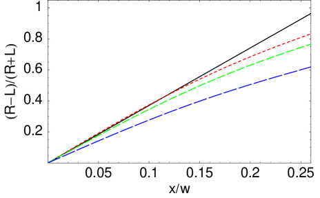
FIG. 7.: Same as Fig. 6, but with $\sigma_{x}/w=0.1$, $\sigma_{y}=0$.

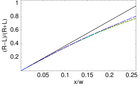
FIG. 8.: Same as Fig. 6, but with $\sigma_{x}=0$, $\sigma_{y}/h=0.1$.

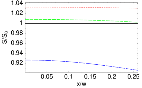
FIG. 9.: Relative magnitude of beam-size corrections in a square chamber with $\sigma_{x}/w=0.1$, $\sigma_{y}/h=0.05$ for three vertical beam offsets $y/h=0,1/8,1/4$ (short-dashed, dashed, long-dashed). Here 1 corresponds to a pencil beam case, i.e. to one of the three curves in Fig. 6 for the corresponding beam vertical offset.

REFERENCES

• [1] J.H. Cuperus, Nucl. Instr. Meth. 145, 219 (1977).
• [2] R.H. Miller, et al., in Proceed. of 12th Int. Conf. on High Energy Accel. (Fermilab, 1983), p. 602.
• [3] S.J. Russel and B.E. Carlsten, in Proceed. of PAC (New York, 1999), p. 477.
• [4] R. Assmann, B. Dehning, and J. Matheson, in Proceed. of EPAC (Vienna, 2000), p. 1693; ibid., p. 412; also in AIP Conf. Proceed. 546, Eds. K.D. Jacobs and R.C. Sibley (New York, 2000), p. 267.
• [5] R.E. Shafer, in AIP Conf. Proceed. 212, Eds. E.R. Beadle and V.J. Castillo (New York, 1990), p. 26.
• [6] S.S. Kurennoy, in AIP Conf. Proceed. 546, Eds. K.D. Jacobs and R.C. Sibley (New York, 2000), p. 283; also S.S. Kurennoy and R.E. Shafer, in Proceed. EPAC (Vienna, 2000), p. 1768.
• [7] S.S. Kurennoy, R.L. Gluckstern, and G.V. Stupakov, Phys. Rev. E 52, 4354 (1995).
• [8] S.S. Kurennoy, in Proceed. EPAC (Sitges, 1996), p. 1449.
Refer to caption