Narrowing of EIT resonance in a Doppler Broadened Medium

Abstract

We derive an analytic expression for the linewidth of EIT resonance in a Doppler broadened system. It is shown here that for relatively low intensity of the driving field the EIT linewidth is proportional to the square root of intensity and is independent of the Doppler width, similar to the laser induced line narrowing effect by Feld and Javan. In the limit of high intensity we recover the usual power broadening case where EIT linewidth is proportional to the intensity and inversely proportional to the Doppler width.

Due to the Doppler effect the atoms in a gas see the radiation field with shifted frequency. Hence the macroscopic polarization representing medium’s response to the radiation, needs to be averaged over the frequency distribution determined by velocity distribution of the atoms. By and large, all sorts of phenomena in gas laser are related to Doppler broadening [1] and it is also the origin of the famous hole burning [2]. and Lamb dip [3, 4]. It was more than thirty years ago that laser induced line narrowing effect in a three-level Doppler broadened system was discovered by Feld and Javan [5]. Notably Feld and Javan found the spectral width of the narrow line to be linearly proportional to the driving field Rabi frequency. Various aspects of this effect have been investigated [6, 7, 8].

The interest to the narrow nonabsorption resonances imposed on the Doppler profile has been resumed recently in a connection with the Electromagnetically Induced Transparency (EIT) experiments which have produced an ultra-slow light propagation [9, 10, 11] with spatial compression (group velocity less than 10’s m/sec) and have made it possible to enhance nonlinear optical processes by orders of magnitude [12, 13, 14, 15].

Steepness of the dispersion function with respect to frequency plays the key role for the small group velocity of light, and is directly related to the transmission width [16, 17, 18]. Hence the behavior of the transmission linewidth in terms of experimental parameters is of a great deal of interest. In high resolution spectroscopy and high precision magnetometry based on a narrow EIT line [19, 20, 21, 22, 23, 24] the experiments are usually carried out with atomic cell configurations so that the effect of Doppler broadening on EIT is also an important concern for the performance of the devices.

Doppler broadening effects in EIT and lasing without inversion (LWI) have been studied in a number of works [25, 26, 27, 28, 29]. Most of these works focused on the possibilities of absorption cancellation and preferable field configurations (co-propagation of probe and drive lasers in folded schemes, counter-propagation in cascade schemes). In the limit of the vanishing probe field and under the assumption that all atoms were trapped to the dark state it was found that the power broadening of EIT line takes place: $\Gamma_{EIT}=\Omega^{2}/W_{D}$ (where $\Omega$ is the Rabi frequency of the driving field and $W_{D}$ is Doppler linewidth), which is similar to the well-known result for the homogeneously broadened system: $\Gamma_{EIT}=\Omega^{2}/\gamma$ (where $\gamma$ is a homogeneous linewidth). This dependence was experimentally verified in [10]. In the limit of relatively low probe field intensity, $\alpha\ll(\gamma/W_{D})\Omega$, and under the same assumption of full coherent trapping (i.e. neglecting by the two-photon coherence decay) it leads to the following result for EIT line width: $\Gamma_{EIT}=\alpha\Omega/\gamma$, where $\alpha$ is the Rabi frequency of the probe field [30].

In this paper, we find an explicit expression for the linewidth of EIT resonance in a Doppler broadened three-level system in the linear approximation with respect to probe field taking into account finite decay time of low-frequency coherence. In the limit of very large intensity it is reduced to the power broadening case. However, for the intermediate range of intensities the coherent population trapping is velocity selective, i.e., it occurs only for those atoms whose frequencies are close to the resonance with a driving field. In this case we find that the width of EIT resonance is proportional to the Rabi frequency of the driving field (similar to result by Feld and Javan [5]) and to the square root of the ratio of the relaxation times of the coherence at the two-photon (low-frequency) and population difference at one-photon (optical) transitions:

$$\Gamma_{EIT} \Longrightarrow ~{}~{}\sqrt{2\gamma_{bc}\over\gamma}~{}\Omega.$$ (1)

This regime corresponds to the narrowest possible EIT line-width and therefore it is very favorable for realization of the efficient EIT-based nonlinear transformations and light storage.

Let us consider the closed atomic model scheme depicted in Fig. 1. In this three-level $\Lambda$ scheme one of the two lower-levels is coupled to the upper level ($a\rightarrow c$) by a coherent drive laser and the transition $a\rightarrow b$ is probed by a weak coherent field. The atomic decays are confined among the given levels. Note that such a model gives a description almost equivalent to the one for an open system in which atoms decay (out of the interaction region) with the rate $\gamma_{bc}$, and atoms are coming into the interaction region with equally populated lower levels. Detailed comparison of our model with the open system will be published elsewhere.

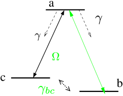
FIG. 1.: Three-level model scheme. The upper level $a$ decays to $b$ and $c$ with decay rate $\gamma$. The relaxation rate between levels $b$ and $c$ is denoted as $\gamma_{bc}$, which is assumed to be small compared to $\gamma$.

If the system is Doppler broadened, the susceptibility should be averaged over the entire velocity distribution such that [1]

$$\chi=\int d(kv)~{}f(kv)~{}\eta\left\{{\rho_{ab}(kv)\over\alpha}\right\},$$ (2)

where $k$ is the wave number of the probe field, $f(kv)$ is the velocity distribution function, $\rho_{ab}(kv)$ is the coherence between states $a$ and $b$ induced by radiation fields, ${\eta\equiv(3/8\pi)N\gamma\lambda^{3}}$, $N$ is the atomic density, and $\lambda$ is the wavelength. For a stationary atom, in the first order of the probe field, $\rho_{ab}$ can be written as

$$\rho_{ab}={-i\alpha\over\Gamma_{ab}\Gamma_{cb}+\Omega^{2}}\Big{[}\Gamma_{cb}(\rho_{aa}^{(0)}-\rho_{bb}^{(0)})+{\Omega^{2}\over\Gamma_{ca}}(\rho_{cc}^{(0)}-\rho_{aa}^{(0)})\Big{]},$$ (3)

where $\rho^{(0)}_{ii}$’s are the zeroth order populations (in the probe field) and ${\Gamma_{ij}\equiv\gamma_{ij}+i\Delta_{ij}}$ with the off-diagonal decay rates $\gamma_{ij}$ given by $\gamma_{ab}=\gamma_{ac}=(\gamma+\gamma^{\prime}+\gamma_{bc})/2$, $\gamma_{cb}=\gamma_{bc}$. $\Delta_{ij}$’s are defined as $\Delta_{ab}=\omega_{ab}-\nu\equiv\Delta$, $\Delta_{ac}=\omega_{ac}-\nu_{0}$, and $\Delta_{cb}=\Delta_{ab}-\Delta_{ac}$, where $\nu$ and $\nu_{0}$ are the frequencies of the probe and drive fields, respectively.

In the present analysis we use the following assumptions: 1) The decay rates in the transitions $a\rightarrow b$ ($\gamma$) and $a\rightarrow c$ ($\gamma^{\prime}$) are assumed to be same ($\gamma$) and defined by spontaneous emission, which is typically the case for the dilute gases. 2) The decay rates of population difference and coherence at the low-frequency transition $b\leftrightarrow c$ are the same ($\gamma_{bc}$), which is typically the case when this decay is determined by the time of flight through the interaction region. 3) The probe field is weak such that the first order analysis is valid. 4) The driving field is on resonance for a stationary atom: $\omega_{ac}=\nu_{0}$. 5) The probe field and driving field propagate in the same direction, and the frequency difference between the transitions $a\rightarrow b$ and $a\rightarrow c$ is small enough such that the residual Doppler shift, $(k-k^{\prime})v$, can be ignored. 6) The EIT condition for the homogeneously broadened system ($\Omega^{2}\gg\gamma\gamma_{bc}$) is valid. 7) The inhomogeneous linewidth ($W_{D}$) is large enough such that $W_{D}\gg\gamma,\Omega$.

Under thses assumptions the atomic populations $\rho^{0}_{ii}$ can be written as

$$\rho_{aa}^{(0)} = {2\gamma_{bc}\Omega^{2}\over 2D},\qquad\rho_{cc}^{(0)}={4\gamma X\gamma_{bc}+2\gamma_{bc}\Omega^{2}\over 2D},$$ (4)

$$\rho_{bb}^{(0)} = {4\gamma X\gamma_{bc}+2\gamma_{bc}\Omega^{2}+2\Omega^{2}\gamma\over 2D},$$ (5)

where $X=[\gamma^{2}+(kv)^{2}]/2\gamma$, and $D=4\gamma X\gamma_{bc}+3\gamma_{bc}\Omega^{2}+\Omega^{2}\gamma$. Then, for an atom with its velocity $v$, the off-diagonal element of the density matrix $\rho_{ab}(kv)$ is found as

$$\rho_{ab} = {i\alpha\over Y}{1\over 2D}\Big{[}\Gamma_{cb}(4\gamma X\gamma_{bc}+2\Omega^{2}\gamma)-\frac{\Omega^{2}4\gamma X\gamma_{bc}}{\gamma+\gamma_{bc}/2+ikv}\Big{]},$$ (6)

where $Y=(\gamma+\gamma_{bc}/2+i\Delta+ikv)(\gamma_{bc}+i\Delta)+\Omega^{2}$.

Doppler broadening is usually modeled by convolution of a given function over a Maxwell-Boltzmann velocity distribution. Due to the complexity in the integration with a Gaussian distribution, however, explanations of the obtained results usually rely on numerical analysis [26, 27, 28, 29]. In order to obtain a simple expression of the linewidth, we approximate the usual Gaussian distribution with a Lorentzian function; this leads to a rather simple form of inhomogeneously broadened susceptibility with which detailed analysis is possible.

If we use a Lorentzian profile as the velocity distribution function $f(kv)$ with full width half maximum (FWHM) $2W_{D}$ such that $f(kv)=(1/\pi)W_{D}/[W_{D}^{2}+(kv)^{2}]$, the Eq. (2) can be evaluated by the contour integration in the complex plane which contains two poles in the lower half plane, viz., $kv=-iW_{D}$ and $kv=-i\sqrt{\Omega^{2}\gamma/2\gamma_{bc}}$. After straight forward calculation of the contributions from the two poles, one can find the complex susceptibility. In particular, the minimum absorption at the line center is obtained as

$$\chi^{\prime\prime}(\Delta=0)={\eta\gamma_{bc}\over\gamma_{bc}W_{D}+\Omega^{2}}\left[{\sqrt{x}\over 1+\sqrt{x}}\right].$$ (7)

where $x={\Omega^{2}\gamma/2\gamma_{bc}W_{D}^{2}}$. We note that, as long as $\Omega^{2}\gg\gamma\gamma_{bc}$, the expression is vanishingly small as $\eta\sqrt{x}/W_{D}$ when $x\ll 1$, and also as $\eta\gamma/W_{D}^{2}$ when $x\gg 1$, so that the EIT (i.e. strong suppression of absorption in the presence of driving field at $\Delta=0$) is preserved. The maximum of $\chi^{\prime\prime}$, on the other hand, can be found as $\chi^{\prime\prime}_{\rm max}\approx\eta/W_{D}$ at $\Delta\approx\pm\Omega$.

Since the absorption at the line center is negligibly small given by (7), we evaluate $\Delta$ which defines $\Gamma_{EIT}$ as $\chi^{\prime\prime}(\Delta=\Gamma_{EIT})=\eta/2W_{D}$. The half width of the EIT resonance ($\Gamma_{EIT}$) is, then, obtained as

$$\Gamma_{EIT}^{2}={\gamma_{bc}\over\gamma}~{}\Omega^{2}(1+x)\left[1+\left\{1+{4x\over(1+x)^{2}}\right\}^{1/2}\right].$$ (8)

This is the main result of the present report. Here we can see the two extreme cases, namely,

$$\Gamma_{EIT} \Longrightarrow ~{}~{}\sqrt{2\gamma_{bc}\over\gamma}~{}\Omega\qquad(x\ll 1),$$ (10)

$$\Longrightarrow ~{}~{}~{}{\Omega^{2}\over W_{D}}\qquad\quad(x\gg 1).$$ (11)

Note that the range of $x$ is: $(\gamma/W_{D})^{2}\ll x\ll\gamma/\gamma_{bc}$. In the expression (10) corresponding to the limit $x\ll 1$, the linewidth of EIT is linearly proportional to $\Omega$, the Rabi frequency of the driving field (i.e., to the square root of the driving field intensity) and it is independent of the Doppler width $W_{D}$.

Similar linear dependence of the linewidth on the Rabi frequency was previously obtained in Ref. [5]. The earlier work [5] dealt with a laser gain system where the weak transitions between the lasing levels were used. The decays out of the lasing levels were the main relaxation mechanisms while the spontaneous decays between levels were not taken into account. These so-called open systems have the relaxation of low-frequency coherence ($\gamma_{bc}$) the same order of magnitude as the relaxation of population difference at the optical transitions ($\gamma$), i.e., $\gamma_{bc}\approx\gamma$. In this case we have $x\approx\Omega^{2}/2W_{D}^{2}$, the Eq. (10) takes a form: $\Gamma_{EIT}\approx\Omega$. Since $\Omega\ll W_{D}$, the linewidth, in turn, is much smaller than $W_{D}$. This limit fully corresponded to experimental conditions of Ref.[5].

In the limit $x\gg 1$ (corresponding to small $\gamma_{bc}$ or a strong driving field) $\Gamma_{EIT}$ is proportional to intensity, $\Omega^{2}$, and inversely proportional to $W_{D}$. Many recent EIT experiments were performed in alkali vapors where the two-photon coherence, ($\rho_{bc}$) was built among the hyperfine levels of the ground state. In these systems the low-frequency coherence relaxation time is determined by the time of flight of the atom through the interaction region, and it is large as compared to the life time of the excited optical state.

In Fig. 2, we plot the EIT linewidth as a function of the Rabi frequency of the driving field. We note that $\Gamma_{EIT}\geq\Omega\sqrt{2\gamma_{bc}/\gamma}$ for any value of $\Omega$. Apparently, smaller ratio $\gamma_{bc}/\gamma$ leads to smaller EIT width at $x\ll 1$, and to smaller value of $\Omega$ at which the linear dependence of $\Omega$ in $\Gamma_{EIT}$ ($\Gamma_{EIT}\propto\Omega$) changes to quadratic dependence ($\Gamma_{EIT}\propto\Omega^{2}$). Both in $x\ll 1$ and $x\gg 1$ limits, for a given value of intensity, the width of EIT resonance in the inhomogeneously broadened medium is smaller than in homogeneously broadened medium with the same homegeneous line width at resonant driving. In the limit $x\gg 1$ this fact was outlined earlier in [30].

FIG. 2.: EIT linewidth (in unit of $\gamma$) as a function of $\Omega$ (also in unit of $\gamma$), with Doppler width $2W_{D}=100\gamma$ and $\gamma_{bc}=10^{-3}\gamma$. The plot (a) of Eq. (8) by averaging over the Lorentzian distribution function (solid line) is almost indistinguishable to that (b) of the numerical result made by Gaussian integration (dotted line). (c) F-J limit denotes the value of $\Omega\sqrt{2\gamma_{bc}/\gamma}$.

This line narrowing effect has a simple physical explanation. Namely, it is due to the reduced power broadening for the off-resonant atoms. At the same time it is worth to note that the width of EIT resonance in Doppler broadened system never can be reduced beyond the ultimate limit defined by low-frequency coherence decay time: $\Gamma_{EIT}\geq\gamma_{bc}$. It reaches this limit when EIT sets in with $\Omega^{2}\geq\gamma\gamma_{bc}$ independently if the optical line is homegeneously or inhomogeneously broadened. In the case $x\gg 1$ EIT line width exceeds this minimum value at least by the factor $W_{D}/\gamma$.

The physical meaning of the parameter $x$ can be understood in the following way: First, let us suppose the system is homogeneously broadened. The optical pumping rate from the level $c$ to $b$ is $\Omega^{2}/\gamma$ for the resonant driving field. In order to have a complete coherent optical pumping in the case of resonant driving this rate should be much bigger than the pumping rate from $b$ to $c$: $\Omega^{2}/\gamma\gg\gamma_{bc}$. This means that the driving field should be sufficiently strong: $\Omega^{2}\gg\Omega_{hom}^{2}\equiv\gamma_{bc}\gamma$. For atoms with velocity $v$, then, the optical pumping rate is $\Omega^{2}\gamma/[\gamma^{2}+(kv)^{2}]$. Then, in order to have a complete coherent optical pumping in a Doppler broadened system we need to require $\Omega^{2}\gamma/(\gamma^{2}+W_{D}^{2})\gg\gamma_{bc}$, which corresponds to $x\gg 1$, i.e., $\Omega^{2}\gg\Omega^{2}_{inhom}\equiv 2\gamma_{bc}W_{D}^{2}/\gamma$. Hence, the parameter $x$ represents the degree of optical pumping from the level $c$ to $b$ within the inhomogeneous line width ($x=\Omega^{2}/\Omega^{2}_{inhom}$).

With a notion of the effective width $\delta_{\rm eff}$, the width of EIT resonance can always be regarded as

$$\Gamma_{EIT}\sim{\Omega^{2}\over\delta_{\rm eff}},$$ (12)

which is equivalent to the EIT linewidth for the homogeneously broadened medium (where $\Gamma_{EIT}=\Omega^{2}/\gamma$). The effective width $\delta_{\rm eff}$ is defined as the magnitude of the maximum detuning for which atoms are optically pumped into the level $b$ (and hence can interact with a probe field) for a fixed value of $\Omega$.

For $\Omega_{hom}\ll\Omega\ll\Omega_{inhom}$, $\delta_{\rm eff}$ can be estimated by $\Omega^{2}(\gamma/\delta_{\rm eff}^{2})\sim\gamma_{bc}$, yielding $\delta_{\rm eff}\sim\sqrt{\Omega^{2}\gamma/\gamma_{bc}}$. Therefore, an increase of intensity of the driving field makes the number of trapped atoms increased, which results, according to Eq. (12), in the linear dependence of EIT resonance width: $\Gamma_{EIT}\sim{\Omega\sqrt{\gamma_{bc}/\gamma}}$ [see, Eq. (10)]. When $\Omega\gg\Omega_{inhom}$ the number of optically pumped atoms is not increased further (since all of them are already optically pumped into the level $b$), so that $\delta_{\rm eff}\sim W_{D}$ yielding $\Gamma_{EIT}=\Omega^{2}/W_{D}$.

It is worth to note that obtained results can be used for description of EIT experiments not only in gaseous media with Doppler broadening but also in solids with the long lived spin coherence, for example, in rare-earth ions doped crystals at low temperature[31] when inhomogeneous line broadening of optical transitions plays a major role while inohomogeneous broadening of the spin transitions is negligible. On the other hand, they are not directly applicable for EIT experiments involving a buffer gas in a cell or paraffin coating since collisions of the operating atoms with the buffer gas or wells can essentially disturb the Doppler velocity distribution.

The authors wish to thank C. J. Bednar, B. G. Englert, M. S. Feld, M. D. Lukin, A. B. Matsko, Yu. Rostovtsev, V. L. Velichansky, A. S. Zibrov for helpful and stimulating discussions. This work was supported by the Office of Naval Research, Defense Advanced Research Projects Agency, Texas Advanced Research Program, and the Air Force Research Laboratories.

REFERENCES

- [1] See, for example, M. Sargent III, M. O. Scully, and W. E. Lamb, Jr., Laser Physics (Addison-Wesley, Reading, MA, 1974).
- [2] W. R. Bennett, Phys. Rev. 126, 580 (1962).
- [3] A. Szoke, A. Javan, Phys. Rev. Lett. 10, 521 (1963).
- [4] R. A. McFarlane, W. R. Bennett, W. E. Lamb, Appl. Phys. Lett. 2, 189 (1963).
- [5] M. S. Field and A. Javan, Phys. Rev. 177, 540 (1969).
- [6] T. Popova, A. Popov, S. Ravtian, and R. Sokolovskii, Zh. Eksp. Teor. Fiz. 57, 850 (1969) [Sov. Phys. JETP Lett. 30, 466 (1970)].
- [7] T. W. Hänsch and P. E. Toschek, Z. Phys. 236, 213 (1970).
- [8] B. J. Feldman and M. S. Feld, Phys. Rev. A 5, 899 (1972).
- [9] L. V. Hau, S. E. Harris, Z. Dutton, and C. H. Behroozi, Nature 397, 594 (1999).
- [10] M. M. Kash, V. A. Sautenkov, A. S. Zibrov, L. Hollberg, G. R. Welch, M. D. Lukin, Y. Rostovtsev, E. S. Fry, and M. O. Scully, Phys. Rev. Lett. 82, 5229 (1999).
- [11] D. Budker, D. F. Kimball, S. M. Rochester, and V. V. Yashchuk, Phys. Rev. Lett. 83, 1767 (1999).
- [12] K. Hakuta, L. Marmet, and B. P. Stoicheff, Phys. Rev. Lett. 66, 596 (1991).
- [13] P. R. Hemmer, D. P. Katz, J. Donoghue, M. Cronin-Golomb, M. S. Shahriar, and P. Kumar, Opt. Lett. 20, 982 (1995).
- [14] M. Jain, H. Xia, G. Y. Yin, A. J. Merriam, and S. E. Harris, Phys. Rev. Lett. 77, 4326 (1996).
- [15] A. S. Zibrov, M. D. Lukin and M. O. Scully, Phys. Rev. Lett. 83, 4049 (1999).
- [16] S. E. Harris, J. E. Field, and A. Kasapi, Phys. Rev. A 46, R29 (1992).
- [17] M. Xiao, Y. Q. Li, S. Z. Jin, and J. Gea-Banacloche, Phys. Rev. Lett. 74, 666 (1995).
- [18] O. Schmidt, R. Wynands, Z. Hussein, and D. Meschede, Phys. Rev. A 53, R27 (1996).
- [19] M. O. Scully and M. Fleischhauer, Phys. Rev. Lett. 69, 1360 (1992).
- [20] M. Fleischhauer and M. O. Scully, Phys. Rev. A 49, 1973 (1994).
- [21] S. Brandt, A. Nagel, R. Wynands, and D. Meschede, Phys. Rev. A 56, R1063 (1997).
- [22] M. D. Lukin, M. Fleischhauer, A. S. Zibrov, H. G. Robinson, V. L. Velichansky, L. Hollberg, and M. O. Scully, Phys. Rev. Lett. 79, 2959 (1997).
- [23] D. Budker, V. Yashchuk, and M. Zolotorev, Phys. Rev. Lett. 81, 5788 (1998).
- [24] A. Nagel, L. Graf, A. Naumov, E. Mariotti, V. Biancalana, D. Meschede, and R. Wynands, Europhys. Lett. 44, 31 (1996).
- [25] See, for example, E. Arimondo, Progress in Optics XXXV 257 (1996), and references therein.
- [26] Y. Li and M. Xiao, Phys. Rev. A 51, R2703 (1995).
- [27] A. Karawajczyk and J. Zakrzewski, Phys. Rev. A 51, 830 (1995).
- [28] G. Vemuri and G. S. Agarwal, Phys. Rev. A 53, 1060 (1996).
- [29] D. Z. Wang and J. Y. Gao, Phys. Rev. A 52, 3201 (1995).
- [30] A. V. Taichenachev, A. M. Tumaikin, and V. I. Yudin, JETP Lett. 72, 173 (2000).
- [31] B. S. Ham, P. R. Hemmer, M. S. Shahriar, Opt.Commun. 144, 227 (1997).