How to Introduce A World Time to A Part of Two Dimensional de Sitter Manifold

Abstract

We define 1+1 dimensional de Sitter manifold in this paper and we consider various coordinate systems on it. Some interesting aspects of the general theory of relativity are demonstrated using the transformations between considered coordinate systems. The problem might be of interest for physics and mathematics students as well as for physics teachers.

1 Introduction

At first we stress the importance of $3+1$ version of de Sitter manifold in relativistic cosmology (inflation) and quantum field theory in curved spacetime. For more details see for example the book of Birrell and Davies [1], more information about the (cosmological) inflation can be found in [2] or in recent papers concerning the inflation. We suppose that the reader of this text is familiar with modern differential geometry. If not see for example the introductory pages of books [3], or [4]. Now let us start with definition:
Def.: 2D de Sitter manifold ($DS^{2}$) is defined by the constraint

$$x^{2}+y^{2}-t^{2}=a^{2}\qquad(a>0)\quad,$$ (1)

as the submanifold of 3D Minkowski space $M^{2+1}_{[t,x,y]}$. Metric structure on $M^{2+1}_{[t,x,y]}$ is given by the flat metric tensor

$$\eta_{3}=dx\otimes dx+dy\otimes dy-dt\otimes dt\quad.$$ (2)

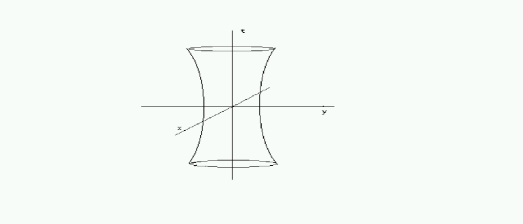
Figure 1: $DS^{2}$ as the submanifold of $M^{2+1}$

So, if we introduce new coordinates ($r,\phi$) to describe $DS^{2}$ by the following equations

$$\begin{array}[]{ccc}x&=&r\cos(\phi)\quad,\\ y&=&r\sin(\phi)\quad,\end{array}\qquad\begin{array}[]{c}r\in[a,\infty)\\ \phi\in[0,2\pi)\quad,\end{array}$$ (3)

then we can write the induced metric tensor $g$ on $DS^{2}$ in the form:

$$g=\frac{a^{2}}{a^{2}-r^{2}}dr\otimes dr+r^{2}d\phi\otimes d\phi\quad.$$ (4)

Looking on the space-time character of vectors $\partial_{r}$ and $\partial_{\phi}$ (i.e. evaluating $g(\partial_{r},\partial_{r})$ and $g(\partial_{\phi},\partial_{\phi}))$ we shall see that the coordinates $\phi$ and $r$ correspond to space coordinate and time coordinate respectively. The cut of $DS^{2}$ by the surface (see fig.1.) $t=const$ is a circle parallel with the $xy$ plane, the radius of the circle is equal to $r=\sqrt{a^{2}+t^{2}}$. Such a cut represents the ordinary space (or space), volume of which is equal to

$$Vol_{1}=2\pi r=2\pi\sqrt{a^{2}+t^{2}}\quad.$$ (5)

Another set of convenient coordinates ($\theta,\phi$) is given by the transformation:

$$r=a\cosh(\theta)\quad,\qquad\theta\in R\quad,$$ (6)

and the $g$ tensor has a form:

$$g=a^{2}\left[-d\theta\otimes d\theta+\cosh^{2}(\theta)d\phi\otimes d\phi\right]\quad.$$ (7)

The last formula expresses that $DS^{2}$ is a two dimensional version of the closed Robertson - Walker inflating Universe. The coordinate $\theta$ plays the role of time and the scale parameter (the radius of the space) evolution is given by

$$a\cosh(\theta)\quad.$$

2 Killing’s vector field on $DS^{2}$

The isometric (continous) transformations of any smooth manifold (especially $DS^{2}$) are generated by some vector field - say $V$. We think by "are generated" that the flow of $V$ is an isometric transformation of the manifold under consideration. Such a vector field $V$ is called the Killing’s vector (vector field). The condition for $V$ to be the Killing’s vector is well known (the Killing’s equation) - see e.g. [1]:

$$\mathcal{L}_{V}g=0\quad,$$ (8)

where $\mathcal{L}_{V}$ is the Lie derivative with respect to $V$. Let us denote $x^{0}=\theta$ and $x^{1}=\phi$ . Then the Killings’ equations for $DS^{2}$ may be written as follows

$$V^{k}g_{ij,k}+V^{k}_{,i}g_{kj}+V^{k}_{,j}g_{ik}=0\qquad(i,j,k\in\{0,1\})\quad,$$ (9)

where $F_{,i}=\partial_{x_{i}}F$, or one can write the same in the $(\theta,\phi)$ coordinates

$$\begin{array}[]{ccc}V^{1}_{,1}&=&0\quad,\\ \sinh(\theta)V^{1}+\cosh(\theta)V^{2}_{,2}&=&0\quad,\\ \cosh^{2}(\theta)V^{2}_{,1}-V^{1}_{,2}&=&0\quad.\end{array}$$ (10)

It is very simple to find the general solution of the system (10). The result is

$$V\equiv V^{1}\partial_{1}+V^{2}\partial_{2}=A\cos(\phi-\phi_{0})\partial_{\theta}-A\tanh(\theta)\sin(\phi-\phi_{0})\partial_{\phi}+B\partial_{\phi},$$ (11)

with $A,B$ and $\phi_{0}$ being real constants. In the old coordinates $(r,\phi)$ we have

$$V=A\cos(\phi-\phi_{0})\sqrt{r^{2}-a^{2}}\partial_{r}-A\sin(\phi-\phi_{0})\frac{\sqrt{r^{2}-a^{2}}}{r}\partial_{\phi}+B\partial_{\phi}\quad.$$

Now, we are going to separate $V$ into two parts and we shall discuss their meaning:
(i.) Let us take

$$V^{rot}=B\partial_{\phi}\quad.$$

It is clear that the flow of $V^{rot}$ makes the rotation of $DS^{2}$ with the velocity $B$ around the $t$ axis. (If $B=0$ then we have the identity transformation.) The space-time character of $V^{rot}$ is given by its length

$$g(V^{rot},V^{rot})=B^{2}g(\partial_{\phi},\partial_{\phi})=B^{2}r^{2}>0\quad.$$ (12)

So $V^{rot}$ is a space-like vector field and the integral curves of this field are not worldlines of any real object.
(ii.) The rest of $V$ is

$$\tilde{V}=A\sqrt{r^{2}-a^{2}}\left(\cos(\phi-\phi_{0})\partial_{r}-\frac{1}{r}\sin(\phi-\phi_{0})\partial_{\phi}\right)\quad.$$

$DS^{2}$ is invariant under the flow of $B\partial_{\phi}$ (i.e. under the rotations around the $t$ axis as was said in (i.)). So we can put $\phi_{0}=0$ without lost of generality. In this case we have

$$\tilde{V}(\phi_{0}=0)=A\sqrt{r^{2}-a^{2}}\partial_{x}\equiv\tilde{V}_{x}\quad.$$

$\tilde{V}_{x}$ represents the (nonuniform) translation along the $x$ axis projected on $DS^{2}$. (In the case of $\phi_{0}\not=0$ $\tilde{V}$ represents analogical translation, but along some axis, which is rotated relatively to the $x$ axis in the $xy$ plane of the background Minkowski space.) Let us look at the space - time character of $\tilde{V}_{x}$

$$g(\tilde{V}_{x},\tilde{V}_{x})=A^{2}(-a^{2}+y^{2})\quad.$$ (13)

We can state that the vector field $\tilde{V}_{x}$ is:
- timelike in the part of $DS^{2}$, in which $|y|<a$
- spacelike in the part of $DS^{2}$, in which $|y|>a$
The part of the space in which the inequality $|y|<a$ holds, consists of two disjoint arcs - see fig.2. The $\phi$ angle, which is defined on fig.2., is given at the moment $t$ as follows:

$$\phi\in[-\alpha,\alpha]\qquad\mbox{if}\quad x>0\quad,$$

$$\phi\in[-\alpha+\pi,\alpha+\pi]\qquad\mbox{if}\quad x<0\quad,$$

where

$$\alpha=\arcsin\left(\frac{a}{r}\right)=\arcsin\left(\frac{a}{\sqrt{a^{2}+t^{2}}}\right)\quad.$$ (14)

3 Motion of light in $DS^{2}$

A smooth curve (worldline) $\gamma\subset DS^{2}$ is isotropic (or lightlike) if and only if

$$g(\dot{\gamma},\dot{\gamma})=0\quad.$$ (15)

A condition equivalent to this one is the following

$$\frac{d\theta}{\cosh(\theta)}=\pm d\phi\quad.$$ (16)

Performing the integration we get the equation of the general isotropic line in $DS^{2}$ in the form

$$\pm\phi=c_{\pm}+2\arctan(e^{\theta})\quad.$$ (17)

This solution can be written in other coordinates as

$$\pm\phi=c_{\pm}+2\arctan\left(\frac{r}{a}+\sqrt{\left(\frac{r}{a}\right)^{2}-1}\right)=c_{\pm}+2\arctan\left(\sqrt{1+\left(\frac{t}{a}\right)^{2}}+\frac{t}{a}\right).$$

The space in $DS^{2}$ is one dimensional, the space coordinate from the doublet $(t,\phi)$ is $\phi$ and $\phi\in[0,2\pi)$. The difference

$$\delta\phi=\phi(t_{2})-\phi(t_{1})\quad,$$

computed with respect to (17), describes the space translation of the light during the time interval between $t_{1}$ and $t_{2}$. If two signals were emitted at the moment $t=0$ from the same point, the first one in the $+\phi$ direction and the second in the $-\phi$ direction, then the two points, that this two signals reach at the time $t>0$, represent the particle horizon relatively to the starting point of the signal emission.
Let us consider the two antiparallel signals emitted from the point $(t=0,\phi=\pi/2)\in DS^{2}$ (see fig.2.). The constant $c$ (see (16)) is equal to $0$, for the signal emitted in $+\phi$ direction, and it is equal to $\pi$, for the signal emitted in the $-\phi$ direction. The signals positions may be characterized by the $\beta$ angle

$$\beta(t)=\phi_{+}(t)-\phi_{+}(0)=2\arctan\left(\frac{t}{a}+\sqrt{\frac{t^{2}}{a^{2}}+1}\right)-\frac{\pi}{2}\quad.$$

One trivially shows that

$$\beta(t)=\frac{\pi}{2}-\alpha(t)\quad.$$

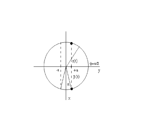
Figure 2: It shows the ordinary space and the particle horizon position (the two marked points) at the moment of time $t$

4 World time

The Killing’s vector field $\tilde{V}_{x}$ is timelike in the part of $DS^{2}$, in which the inequality $|y|<a$ is satisfied. It is possible to introduce there local coordinates so that the coefficients of the metric tensor do not depend on the time. One speaks about the world time. We note, that this part of $DS^{2}$ is assigned (fig.2.) by the $\alpha$ angle given by (14) or as well as by $\beta$ angle and the physical meaning of these angles was discussed in the previous sections.
In the area, which is now under consideration, we have

$$x^{2}-t^{2}=a^{2}-y^{2}\equiv Y^{2}>0\quad.$$ (18)

So we can introduce the new coordinates $(Y,T)$ by the following relations

$$\begin{array}[]{ccc}x&=&Y\cosh(T)\quad,\\ t&=&Y\sinh(T)\quad,\end{array}\qquad\begin{array}[]{ccc}Y&\in&[-a,a]\quad,\\ T&\in&R\quad.\end{array}$$ (19)

The metric tensor has the form

$$g=\frac{a^{2}}{a^{2}-Y^{2}}dY\otimes dY-Y^{2}dT\otimes dT\quad.$$ (20)

We see that we have presented a part of $DS^{2}$ as a static spacetime and that the $T$ coordinate plays the role of the world time.
What is the volume of the space (as a function of time) for an observer measuring the space-time distances according to the formula (20)? The space part of the metric tensor (19) is given by

$$\hat{g}=\sqrt{|\det(g)|}dY=\frac{a}{\sqrt{a^{2}-Y^{2}}}dY\quad,$$

so we get the volume in question as follows

$$Vol_{2}=a\int_{-a}^{+a}\frac{dY}{\sqrt{a^{2}-Y^{2}}}=\pi a\quad.$$ (21)

We note that there are two (for all $t\not=0$) disjoint parts of $DS^{2}$, in which the world time can be introduced. The volume of both of them is given by the previous formula.

5 Relativity of space infinity

Now let us consider the part of $DS^{2}$, in which the inequality $|y|>a$ holds.We can write

$$x^{2}-t^{2}=a^{2}-y^{2}\equiv-Z^{2}<0\quad,$$ (22)

an we can make an analogical transformation of the coordinates as in the previous section

$$\begin{array}[]{ccc}x&=&Z\sinh(\rho)\quad,\\ t&=&Z\cosh(\rho)\quad,\end{array}\qquad\begin{array}[]{ccc}Z&\in&R\quad,\\ \rho&\in&R\quad.\end{array}$$ (23)

Tensor $g$ expressed in $(Y,\rho)$ coordinates becomes

$$g=-\frac{a^{2}}{a^{2}+Z^{2}}dZ\otimes dZ+Z^{2}d\rho\otimes d\rho\quad.$$ (24)

The last expression for $g$ suggests us to make one more transformation

$$Z=a\sinh(\tau)\quad,\qquad\tau\in R\quad,$$ (25)

and to express $g$ in terms of the pair $(\tau,\rho)$

$$g=a^{2}\left[-d\tau\otimes d\tau+\sinh^{2}(\tau)d\rho\otimes d\rho\right]\quad.$$ (26)

It is clear that the $\tau$ coordinate plays the role of time now and that we have just presented this part of $DS^{2}$ as the two dimensional version of the open Robertson-Walker inflating Universe with the scale parameter evolution given by

$$a\sinh(\tau)\quad.$$

The following formula

$$\hat{g}=\sqrt{|\det(g)|}d\rho=a\sinh(\tau)d\rho\quad.$$

gives the metrics on the hyperplane (the curve) $\tau=const.$. It implies that the volume of space is given at the moment $\tau$ by

$$Vol_{3}=a\sinh(\tau)\int_{-\infty}^{\infty}d\rho\quad.$$ (27)

We can see that this volume is infinite for all $\tau\not=0$.

6 Conclusion

We have started from the de Sitter manifold, which is a special case of the closed Robertson-Walker Universe. Then we have presented, using the suitable coordinate transformation (19), well defined part of it as the static Universe, i.e. we have introduced on that part of $DS^{2}$ the world time. One can discover on this example, that the determination of the arrow of time, using the expansion of the Universe, might be problematic. Thereafter we used other coordinate transformations - eqs. (23) and (25) - and we presented the part of $DS^{2}$ as the open Robertson-Walker Universe. The motivation and the interpretation for these coordinate transformations is given by the analysis of the Killing’s vector field od $DS^{2}$ and the motion of light in $DS^{2}$, that we have done in the second and third sections. The idea to present a part of closed inflating Universe as an open inflating Universe has a great use in the cosmology, especially in the scenarios of evolution of the very early Universe. From the physical point of view the inflating Universe (as $DS^{2}$) is an Universe filled by the homogenous configuration of a scalar field with the positive energy density. This idea was presented in the work [5]. It leads to the possibility of "the quantum creation of an open Universe" - see for example [2] or the short paper [6].

References

- [1] N.D.Birrell, P.C.W.Davies: Quantum Fields in Curved Space, Camb. Univ. Press, 1982;
- [2] A.D.Linde: Particle Physics and Inflationary Cosmology, Harwood, Chur, Switzerland, 1990;
- [3] S.Chandrasekhar: The Mathematical Theory of Black Holes, Oxford Univ. Press, Oxford, 1982;
- [4] M.Fecko: Differential Geometry for Physicists, to be published, Bratislava 2002 (in slovak only);
- [5] S. Coleman, F. de Luccia: Phys. Rev. D 21, 1980;
- [6] A.D. Linde: Phys. Rev. D 59, 1999;