Electrodynamics of quasi-periodic media

Abstract

In this work the interaction of electromagnetic field with quasi-periodic media has been scrutinized. We have obtained the formula for a distorted medium polarizability tenzor in the X-ray frequency band. Also there have been obtained the X-rays dynamic diffraction equations for the mediums with arbitrary smooth distortion. For these equations the Takagi-Tuipin equations are obtained as a particular case. We have got a very simple formula for the coefficient of X-rays reflection on the bent Bragg mirror. We have scrutinized the example of calculating the X-rays reflection and focusing by the bent Bragg mirror. Also in this work one could find the rezults of calculating the reflected X-rays caustics form. It is shown that there exists a possibility of linear dimensions of the X-rays focusing area having typical values of $10^{-7}cm$.

I INTRODUCTION

In this article we consider interaction of electromagnetic field with quasi-periodic media which we define as media obtained by some smooth deformation of perfect periodic structures. Mathematically, the term ”smooth deformation” means the biunivocal smooth mapping of the medium under consideration on the medium with perfect periodic structure. The main goal of this article is to show that the electrodynamics of quasi-periodic media can be reduced to the electrodynamics of the perfect periodic media, and, thus, to make possible application to quasi-periodical structures of well-developed classical approaches.The correspondence between perfect  and quasi-periodical media is possible when the later one is considered as the Riemannian manifold with the fundamental metric tensor $\displaystyle g_{\alpha\beta}=$ $\displaystyle\delta_{\alpha\beta}+2\varepsilon_{\alpha\beta}$, where $\displaystyle\delta_{\alpha\beta}$ is the Kronecker symbol and $\displaystyle\varepsilon_{\alpha\beta}$ is the deformation tensor. To clarify this statement, let us remind, that in the mechanics of continuous medium there are two methods describing the deformation processes: the Euler method and the Lagrange method. The co-ordinates coincide with the observer’s frame of reference in the Euler method. The method of Lagrange stands that the co-ordinates are mounted into a medium and are deformed together with a medium. It should be emphasized that the co-ordinates of some point of a medium in the Lagrange co-ordinate system remain unchanged during the medium deformation, whereas the co-ordinates of some point of the medium in the Euler co-ordinate system are being changed. In particular, the co-ordinates of Bravais lattice points of a medium with perfect periodic structure, defined before the deformation by a set of three integers $\displaystyle{\bf n}=\{n_{1},n_{2},n_{3}\}$ will remain constant both during the deformation and after the deformation. Hence, the Bravais lattice of a deformed (quasi-periodic) medium will look alike in the Lagrange and the Euler co-ordinate systems. However, it is necessary to remember, that the area engaged in a quasi-periodic medium in the Lagrange co-ordinate system is a Riemannian manifold with the fundamental metric tensor varying from point to point.

Let us give some examples how the formalism developed in this article can be used while describing the interaction of electromagnetic field with media. Generally even perfect crystals can be referred rather to the quasi-periodic media, than to the media with perfect periodic structure because there are always temperature fields of deformation at least. The classic and quantum superlattices electrodynamics of semiconductors also can be referred to the electrodynamics of the quasi-periodic media when it is necessary to take into account the fields of the deformation, permanently existing in such structures. A big amount of articles devoted to the electrodynamics of the carbonic nanotubes is now published. In most cases they take into the consideration the perfectly straight nanotubes with the perfect periodic structure. Actually there are always some kinds of the nanotube deformation. It is possible to reduce the electrodynamics of such nanotubes, and furthermore the electrodynamics of ensemble of nanotubes in some matrix completely to the electrodynamics of the quasi-periodic media. In real crystals the ensemble of the flaws, dislocations and impurities creates a field of deformations, which is usually divided on two parts. The first one is the averaging over the ensemble and is the smooth field of deformations. The second one describes the fluctuations of the deformations field in comparison with this smooth averaged field. The interaction of an electromagnetic field with the crystals, that have the deformation field being the averaged smooth field of deformations, can be described by methods suggested in this article.

The last example to be considered is the X-ray diffraction optics of the elastically deformed perfect crystals. Such crystals completely correspond to the definition of quasi-periodic media given above. From the point of view of the classical electrodynamics, the X-ray diffraction optics is a simple version of the geometrical optics. The only complication are coupled waves inside a crystal which appear because of the dynamic diffraction. Despite the distorted Bragg mirror is one of the most important parts of almost all X-ray optics system, we have not seen papers correctly describing a dynamic X-rays diffraction on elastically deformed crystals with mean radius of curvature less or about $\displaystyle 10m$ whereas elastically deformed crystals with such media radiuses of curvature are of practical interest. Takagi-Taupin equations [1]-[2] and the series of articles (see bibliography), using this equations as the basic ones are valid for elastically deformed crystals with mean radius of curvature more than $\displaystyle 40m$, as will be shown in part 4. Furthermore, these papers and also paper [5], do not show the difference between two methods describing the crystal deformation mentioned above (Euler and Lagrange methods). The fact is also ignored that the deformed crystal in the Lagrange co-ordinate system is the Riemannian manifold with a fundamental metric tensor varying from point to point in the crystal. Such disregardings lead to a paradoxical statement, that it is impossible to destinguish a perfect crystal and the deformed crystal in the experiments on X-ray beam passing through a crystal far away from the Bragg condition. That contradicts both daily practice of X-ray beams application and classical electrodynamics because the deformed crystal is a nonuniform medium with refraction index and absorption coefficient depending on co-ordinates.

The first section of this article is dedicated to the electrodynamics of media with perfect periodic structure and is being auxiliary. As the medium with periodic structure is a medium with a spatial dispersion and the relation between the vector of polarization and the electric vector is not local, the wave equation is the integro-differential one and is rather difficult to work with. In case of media with perfect periodic structure one usually proceeds to the ($\displaystyle k,\omega$)-representation, where the integro-differential wave equation is replaced by the system of the algebraic equations. Then one derives the medium eigenmodes from the dispersion equation and gains all key results of the electrodynamics of media with perfect periodic structure. Such an algorithm defies the quasi-periodic media generalization, therefore in the first section we expound an unknown method, unwieldy and inconvenient on the first sight, that allows to substitute the integro-differential wave equation for the equivalent system of the differential equations, that describes the electromagnetic field dynamic diffraction by the media with perfect periodic structure. This method can be naturally generalized for the case of the quasi-periodic media.

The second section is devoted to the electrodynamics of quasi-periodic media. Proceeding to the Lagrange co-ordinate system allows us to apply the formalism of media with perfect periodic structure developed in the first section to the quasi-periodic media almost without changes in case we consider a quasi-periodic medium in a Lagrange co-ordinate system being a Riemannian manifold.

In the third section we obtain the polarization tensor of a deformed crystal in the X-ray frequency band from the first principles by the joint solution of Maxwell equations and von Neumann’s equation for a density matrix of a crystal. It is necessary to underline here, that the dependence of the Debye-Waller factor on the co-ordinates is ignored, the Fourier-components of the polarization tensor of a deformed crystal coincide with Fourier-components of the polarization tensor of a perfect crystal by the shape only in a Lagrange co-ordinate system. These components appear to be very complicated co-ordinate functions in the observer system (Euler co-ordinate system).

In the fourth section we obtain the equations system of the two-wave X-rays diffraction on the deformed crystals and after a series of simplifying approximations we show that it is possible to receive from these equations a combined Takagi -Taupin [1]-[2] equations system which appears applicable only for the deformations of the crystals with medial radius of curvature more than $\displaystyle 40m$ .

Finally in the fifth section we use a principle of the geometrical optics locality to offer a simple formula for the Bragg reflection coefficient from distorted Bragg mirror and describe the X-ray quanta mirror focusing.

II Perfect periodic structures

First we consider interaction of the electromagnetic field with a perfect periodic medium. For media with spatial dispersion, the wave equation for electric field vector in $\displaystyle\omega$-representation has the form as follows:

$$rotrot{\bf E}({\bf r},\omega)=\frac{\omega^{2}}{c^{2}}{\bf E}({\bf r},\omega)+\frac{\omega^{2}}{c^{2}}\int d^{3}{\bf r}^{\prime}\hat{\chi}({\bf r},{\bf r}^{\prime};\omega){\bf E}({\bf r}^{\prime},\omega)+\frac{4\pi\omega i}{c^{2}}{\bf j}^{(e)}({\bf r},\omega)$$ (1)

where $\displaystyle\hat{\chi}({\bf r},{\bf r}^{\prime};\omega)$ is the medium polarization tensor, and $\displaystyle{\bf j}^{(e)}({\bf r},\omega)$ is the current density of external sources. The intrinsic property of perfect periodic media to be translationally invariant, makes it possible to expand the polarizability tensor into the Fourier series:

$$\hat{\chi}({\bf r},{\bf r}^{\prime};\omega)=\hat{\chi}({\bf r}+{\bf R}_{{\bf n}},{\bf r}^{\prime}+{\bf R}_{{\bf n}};\omega)=\hat{\chi}({\bf r}-{\bf r}^{\prime},{\bf r}^{\prime};\omega)=\sum\limits_{{\bf l}}\hat{\chi}^{{\bf l}}({\bf r}-{\bf r}^{\prime};\omega)\exp\left\{-i\left\langle{\bf\tau}^{({\bf l})},{\bf r}^{\prime}\right\rangle\right\}$$ (2)

In the above equations $\displaystyle{\bf R}_{{\bf n}}=n_{1}{\bf a}_{1}+n_{2}{\bf a}_{2}+n_{3}{\bf a}_{3}$ is the Bravais lattice vector, $\displaystyle{\bf n}=\{n_{1},n_{2},n_{3}\}$ and $\displaystyle{\bf l}=\{l_{1},l_{2},l_{3}\}$ are integer quantities, $\displaystyle{\bf\tau}^{({\bf l})}=l_{1}{\bf b}_{1}+l_{2}{\bf b}_{2}+l_{3}{\bf b}_{3}$ are the reciprocal lattice vectors, $\displaystyle{\bf a}_{1}$, $\displaystyle{\bf a}_{2}$ , $\displaystyle{\bf a}_{3}$ and $\displaystyle{\bf b}_{1},{\bf b}_{2},{\bf b}_{3}$ are the basic vectors of the Bravais and reciprocal lattices, correspondingly.

Let an electromagnetic wave be incident on a periodic medium with a given Bravais lattice. If the wavelength of the incident electromagnetic field is of the order of the elementary sell linear extension, solution of Eq. (1) is reasonable to seek in the form of the expansion

$${\bf E}({\bf r},\omega)=\sum\limits_{{\bf l}}{\bf E}_{{\bf l}}({\bf r},\omega)e^{i({\bf k}+{\bf\tau}^{({\bf l})}){\bf r}}$$ (3)

where the amplitudes $\displaystyle{\bf E}_{{\bf l}}({\bf r},\omega)$ vary slowly in the area with the linear dimensions less then the wavelength and $\displaystyle({\bf k})^{2}=\frac{\omega^{2}}{c^{2}}$. By substitution Eqs. (2)-(3) into Eq. (1) we obtain

$$\sum\limits_{{\bf l}}e^{i{\bf\tau}^{({\bf l})}{\bf r}}\{\hat{L}[({\bf k}+{\bf\tau}^{({\bf l})}),\nabla]{\bf E}_{{\bf l}}({\bf r},\omega)+k^{2}\sum\limits_{{\bf l}^{\prime}}\int d^{3}{\bf r}^{\prime}\hat{\chi}^{{\bf l}^{\prime}}({\bf r}^{\prime},\omega)e^{-i({\bf k}+{\bf\tau}^{({\bf l})}){\bf r}^{\prime}}{\bf E}_{{\bf l+l}^{\prime}}({\bf r}-{\bf r}^{\prime},\omega)=0$$ (4)

where $\displaystyle{\bf j}^{(e)}({\bf r},\omega)=0$ and the differentiation operator $\displaystyle\hat{L}[({\bf k}+{\bf\tau}^{({\bf l})}),\nabla]$ is determined by

$\displaystyle\displaystyle\hat{L}[({\bf k}+{\bf\tau}^{({\bf l})}),\nabla]=\left[\nabla+i\left({\bf k}+{\bf\tau}^{({\bf l})}\right)\right]\times\left[\nabla+i\left({\bf k}+{\bf\tau}^{({\bf l})}\right)\right].$

The symbol $\displaystyle\times$ stands for the vector product. Expanding the amplitude $\displaystyle{\bf E}_{{\bf l+l}^{\prime}}({\bf r}-{\bf r}^{\prime},\omega)$ into the Taylor series and substituting this series into the integral in expression ( 4) we obtain

$\displaystyle\int d^{3}{\bf r}^{\prime}\hat{\chi}^{{\bf l}^{\prime}}({\bf r}^{\prime},\omega)e^{-i({\bf k}+{\bf\tau}^{({\bf l})}){\bf r}^{{}^{\prime}}}{\bf E}_{{\bf l+l}^{\prime}}({\bf r}-{\bf r}^{\prime},\omega)=\hat{\chi}^{{\bf l}^{\prime}}({\bf k}+{\bf\tau}^{({\bf l})},\omega){\bf E}_{{\bf l+l}^{\prime}}({\bf r},\omega)+$

$\displaystyle i{\displaystyle{\frac{\partial}{\partial k_{i}}}}\hat{\chi}^{{\bf l}^{\prime}}({\bf k}+{\bf\tau}^{({\bf l})},\omega){\displaystyle{\frac{\partial{\bf E}_{{\bf l+l}^{\prime}}({\bf r},\omega)}{\partial x^{i}}}}-\frac{1}{2}{\displaystyle{\frac{\partial}{\partial k_{i}\partial k_{j}}}}\hat{\chi}^{{\bf l}^{\prime}}({\bf k}+{\bf\tau}^{({\bf l})},\omega){\displaystyle{\frac{\partial^{2}{\bf E}_{{\bf l+l}^{\prime}}({\bf r},\omega)}{\partial x^{i}\partial x^{j}}}}+\cdots$.

Here and below, the summation over repetitive indices is implicit. Since $\displaystyle\chi_{\alpha,\beta}^{{\bf ll^{\prime}}}=O(1/k^{2})$, the estimate $\displaystyle[\chi_{\alpha,\beta}^{{\bf ll^{\prime}}}]^{-1}\partial\chi_{\alpha,\beta}^{{\bf ll^{\prime}}}/\partial k_{i}=O(1/k)$ holds true and, as a result, $\displaystyle\partial\chi_{\alpha,\beta}^{{\bf ll^{\prime}}}/\partial k_{i}=o(\chi_{\alpha,\beta}^{{\bf ll^{\prime}}})$. Then, in view of that the amplitudes $\displaystyle{\bf E}_{{\bf l+l}^{\prime}}({\bf r},\omega)$ are slowly varying functions, all terms in the last expression except the first one can be omitted and, consequently, integro-differential equation (4) reduces to

$$\sum\limits_{{\bf l}}e^{i{\bf\tau}^{({\bf l})}{\bf r}}\{\hat{L}[({\bf k}+{\bf\tau}^{({\bf l})}),\nabla]{\bf E}_{{\bf l}}({\bf r},\omega)+k^{2}\sum\limits_{{\bf l}^{\prime}}\hat{\chi}^{{\bf l}^{\prime}}({\bf k}+{\bf\tau}^{({\bf l})},\omega){\bf E}_{{\bf l+l}^{\prime}}({\bf r},\omega)\}=0.$$ (5)

Let $\displaystyle{\bf r}_{0}$ be the radius-vector of the elementary sell center. In that case, any point $\displaystyle{\bf r}$ inside the sell is given by $\displaystyle{\bf r}={\bf r}_{0}+{\bf\eta}$. Taking this representation into account, let us multiply the last equation by $\displaystyle\exp\{-i{\bf\tau}^{({\bf l})}{\bf r}\}$ and integrate the product over the elementary sell volume $\displaystyle\Omega$:

$$\displaystyle\sum\limits_{{\bf l}^{\prime}}e^{i({\bf\tau}({\bf l}^{\prime})-{\bf\tau}^{({\bf l})}){\bf r}_{0}}\{\int\limits_{\Omega}e^{i({\bf\tau}({\bf l}^{\prime})-{\bf\tau}^{({\bf l})}){\bf\eta}}\hat{L}[({\bf k}+{\bf\tau}({\bf l}^{\prime})),\nabla]{\bf E}_{{\bf l}^{\prime}}({\bf r}_{0}+{\bf\eta},\omega)d^{3}{\bf\eta}$$ (6)

$$\displaystyle+k^{2}\sum\limits_{{\bf l}^{{}^{\prime\prime}}}\hat{\chi}^{{\bf l}^{{}^{\prime\prime}}}({\bf k}+{\bf\tau}({\bf l}^{\prime}),\omega)\int\limits_{\Omega}e^{i({\bf\tau}({\bf l}^{\prime})-{\bf\tau}^{({\bf l})}){\bf\eta}}{\bf E}_{{\bf l}^{\prime}{\bf+l}^{{}^{\prime\prime}}}({\bf r}_{0}+{\bf\eta},\omega)d^{3}{\bf\eta}\}=0$$ (7)

In the framework of the slowly varying amplitude approximation taken above, the quantities $\displaystyle\hat{L}[({\bf k}+{\bf\tau}(l^{{}^{\prime}})),\nabla]{\bf E}_{{\bf l}^{\prime}}({\bf r}_{0}+{\bf\eta},\omega)$ and$\displaystyle{\bf E}_{{\bf l}^{\prime}{\bf+l}^{{}^{\prime\prime}}}({\bf r}_{0}+{\bf\eta},\omega)$ can be treated as constants within the elementary sell and, thus, can be factored out from the integrals. In that case, since

$\displaystyle\displaystyle\ \int\limits_{\Omega}e^{i({\bf\tau}({\bf l}^{\prime})-{\bf\tau}^{({\bf l})}){\bf\eta}}d^{3}{\bf\eta}=\Omega\delta_{{\bf l,l}^{\prime}}$

the equation (5) reduces to the system as follows:

$$\hat{L}[({\bf k}+{\bf\tau}^{({\bf l})}),\nabla]{\bf E}_{{\bf l}}({\bf r},\omega)+k^{2}\sum\limits_{{\bf l}^{\prime}}\hat{\chi}^{{\bf l}^{\prime}}({\bf k}+{\bf\tau}^{({\bf l})},\omega){\bf E}_{{\bf l+l}^{\prime}}({\bf r},\omega)=0$$ (8)

Together with Eq. (3), this equation system describes the electromagnetic field dynamic diffraction by a perfect periodic medium.

When the wavelength is much larger then the medium unit cell linear size, electromagnetic fields propagating in the medium can be averaged over the elementary sell and, then, a hypotatic homogeneous medium with effective constitutive parameters can be introduced into consideration instead of the real inhomogeneous one. Polarization of this homogeneous medium is related to averaged electromagnetic field by $\displaystyle{\bf P}_{avg}({\bf r},\omega)=\hat{\chi}_{avg}{\bf E}_{avg}({\bf r},\omega)$, where $\displaystyle\hat{\chi}_{avg}$ is the polarization tensor which determines the linear electromagnetic response of the effective homogeneous medium.  In accordance with [7], the effective polarizability tensor $\displaystyle\hat{\chi}^{avg}({\bf k};\omega)$ is expressed in terms of the Fuorier transform of the microscopic polarizability tensor (2) by

$$\hat{\chi}^{avg}({\bf k};\omega)=\hat{\chi}^{{\bf 0}}({\bf k};\omega)\frac{1}{1+\hat{N}\hat{\chi}^{{\bf 0}}({\bf k};\omega)}$$ (9)

The tensor $\displaystyle\hat{N}$  takes into account interaction between scattering centers and is determined by the lattice geometry:

$$\displaystyle\hat{N} \displaystyle= \displaystyle\lim_{{\bf r}\rightarrow{\bf R}_{{\bf m}}}({\rm graddiv}+\varkappa^{2})\int\limits_{\Omega}d^{3}{\bf\eta}^{\prime}\frac{e^{-i\varkappa\mid{\bf r}-{\bf R}_{{\bf m}}-{\bf\eta}^{\prime}\mid}}{\mid{\bf r}-{\bf R}_{{\bf m}}-{\bf\eta}^{\prime}\mid}\varphi({\bf\eta}^{{}^{\prime}})\thickapprox$$ (11)

$$\displaystyle\lim\limits_{{\bf r}\rightarrow{\bf R}_{{\bf m}}}{\rm graddiv}\int\limits_{\Omega}d^{3}{\bf\eta}^{\prime}\frac{\varphi({\bf\eta}^{\prime})}{\mid{\bf r}-{\bf R}_{{\bf m}}-{\bf\eta}^{\prime}\mid}$$

The function $\displaystyle\varphi({\bf\eta})$  is an even function of co-ordinates. In centro-symmetrical lattices it is defined by its momenta:

$$\frac{1}{\Omega}\int\limits_{\Omega}d^{3}{\bf\eta}\varphi({\bf\eta})=1,\frac{1}{\Omega}\int\limits_{\Omega}d^{3}{\bf\eta}\eta^{i}\varphi({\bf\eta})=0,\frac{1}{\Omega}\int\limits_{\Omega}d^{3}{\bf\eta}\eta^{i}\eta^{j}\varphi({\bf\eta})=\delta^{ij},\cdots.$$ (12)

The tensor $\displaystyle\hat{N}$ has been evaluated analytically for some types of elementary cells [7]. In other cases it can be done numerically.

III Quasi-periodic structures

The basic assumption which the procedure of derivation of Eqs. (8)-( 11) leaned upon, is the relation (3) accounting for the property of the polarizability tensor of perfect periodic structures to be translationally invariant. Under effect of deformation, this invariance, e.g. condition (3), is disrupted and thus the algorithm of Eqs. (8)-(9) derivation outlined above becomes invalid. However, an appropriate modification based on the approach originated from the continuous medium mechanics can be applied to involve deformed periodic media into consideration. In the mechanics of continuous media there are two alternative methods of the deformation process description, the Euler method and the Lagrange method. In the framework of the first one the co-ordinate system is coupled with the viewpoint whereas the second method treats the co-ordinate system frozen into the medium and, thus, in the process of deformation the co-ordinate lines are transformed along with the medium. As a result, the Euler co-ordinates of a given point $\displaystyle x^{i}$ are changed during the deformation whereas the Lagrange co-ordinates of it, $\displaystyle\xi^{i}$, remain fixed. Lagrange and Euler co-ordinates are related to one another by

$$x^{i}=\xi^{i}+u^{i}(\xi^{1},\xi^{2},\xi^{3});\quad i=1,2,3\,,$$ (13)

where $\displaystyle u^{i}(\xi^{1},\xi^{2},\xi^{3})$ stand for the deformation field components. In particular, choosing the co-ordinate system $\displaystyle{\bf e}_{i}$ to be related to the elementary translation vectors of the Bravais lattice $\displaystyle{\bf a}_{i}$, $\displaystyle{\bf e}_{i}={\bf a}_{i}/|{\bf a}_{i}|$, we find out the Lagrange co-ordinates of the Bravais lattice sites to be given by quantities $\displaystyle\xi_{{\bf n}}=\{n_{1}a_{1},n_{2}a_{2},n_{3}a_{3}\}$ both before and after the deformation. Thus, one can conclude that in the Lagrange co-ordinates, the Bravais lattice of a deformed periodic structure looks like to the Bravais lattice of a perfect periodic structure and consequently, the polarizability tensor in the Lagrange co-ordinates proves to be translationally invariant. This allows us to state the relations as follows

$$\hat{\chi}({\bf\xi},{\bf\xi}^{\prime};\omega)=\hat{\chi}({\bf\xi}+{\bf\xi}_{{\bf n}},{\bf\xi}^{\prime}+{\bf\xi}_{{\bf n}};\omega)=\hat{\chi}({\bf\xi}-{\bf\xi}^{\prime},{\bf\xi}^{\prime};\omega)=\sum\limits_{{\bf l}}\hat{\chi}^{{\bf l}}({\bf\xi}-{\bf\xi}^{{}^{\prime}};\omega)\exp\left\{-i\left\langle{\bf\tau}^{({\bf l})},{\bf\xi}^{\prime}\right\rangle\right\}$$ (14)

where $\displaystyle{\bf\tau}^{({\bf l})}=\{{2\pi l_{1}/a_{1}},{2\pi l_{2}/a_{2}},{2\pi l_{3}/a_{3}}\}$ is the reciprocal lattice covector in the Lagrange co-ordinate system; its components in the Euler co-ordinates are defined by $\displaystyle\tau_{{\bf l}i}({\bf r})=(2\pi l_{j}/a_{j}){\partial\xi^{j}}/{\partial x^{i}},~{}i=1,2,3\,.$. It should be emphasized that, mathematically, a deformed medium is the Riemann manifold with the fundamental metric tensor as follows

$\displaystyle\displaystyle g_{ij}(\xi^{1},\xi^{2},\xi^{3})=g_{ij}^{0}+2\varepsilon_{ij}(\xi^{1},\xi^{2},\xi^{3})$

where $\displaystyle\varepsilon_{ij}(\xi^{1},\xi^{2},\xi^{3})$ is the deformation tensor of the medium:

$$\varepsilon_{ij}(\xi^{1},\xi^{2},\xi^{3})=\frac{1}{2}(g_{ik}^{0}\frac{\partial u^{k}}{\partial\xi^{j}}+g_{jk}^{0}\frac{\partial u^{k}}{\partial\xi^{i}}+g_{lk}^{0}\frac{\partial u^{l}}{\partial\xi^{j}}\frac{\partial u^{k}}{\partial\xi^{i}})$$ (15)

Here $\displaystyle g_{ij}^{0}=({\bf e}_{i}\cdot{\bf e}_{j})$ is the metric tensor of elementary cell of the perfect periodic medium. Further mathematical analysis accounted for the properties of the Riemann manifolds allows one to extend the approach being developed to media which need not be obtained by deformation of the perfect periodic medium. In order for relation (13) to hold true, a one-to-one smooth mapping (14) of the medium being considered into a perfect periodic structure is necessary and sufficient to exist. The media for which such a mapping exists we shall refer to as quasi-periodic media. Wave equation for quasi-periodic media in the Lagrange co-ordinates takes the form as follows

$$\displaystyle[e_{h}({\bf\xi})\otimes g^{kh}{\displaystyle{\frac{\partial}{\partial\xi^{k}}}}\frac{1}{\sqrt{g}}{\displaystyle{\frac{\partial}{\partial\xi^{l}}}}\sqrt{g}e^{l}({\bf\xi})-\frac{1}{\sqrt{g}}{\displaystyle{\frac{\partial}{\partial\xi^{l}}}}\sqrt{g}g^{kl}{\displaystyle{\frac{\partial}{\partial\xi^{k}}}}]{\bf E}({\bf\xi},\omega)=\frac{\omega^{2}}{c^{2}}{\bf E}({\bf\xi},\omega)$$ (16)

$$\displaystyle+\frac{\omega^{2}}{c^{2}}\sum\limits_{{\bf l}}\int d^{3}{\bf\xi}^{\prime}\sqrt{\left|g({\bf\xi}^{\prime})\right|}\hat{\chi}^{{\bf l}}({\bf\xi}-{\bf\xi}^{\prime};\omega)e^{-i\tau_{i}^{({\bf l})}\xi^{i}}{\bf E}({\bf\xi}^{\prime},\omega)+\frac{4\pi\omega i}{c^{2}}{\bf j}^{(e)}({\bf\xi},\omega)$$ (17)

where $\displaystyle g^{ij}(\xi)$ is the tensor inverse to the metric tensor $\displaystyle g_{ij}(\xi)$ determined by Eq. (15)  ($\displaystyle g^{ij}(\xi)g_{jk}(\xi)=\delta_{k}^{i}$),  $\displaystyle g(\xi)=\det\left\|g_{ij}({\bf\xi})\right\|.$

The procedure of derivation of basic equation describing wave diffraction by quasi-periodic media is analogous to that applied above under derivation of Eqs. (8)-(9). As in the case of perfect periodic media, solution of wave equation (17) we shell seek in the form of expansion analogous to (3):

$${\bf E}({\bf\xi},\omega)=\sum\limits_{{\bf l}}{\bf E}_{{\bf l}}({\bf\xi},\omega)e^{i[k_{i}+\tau_{i}^{({\bf l})}]\xi^{i}+ik_{i}u^{i}({\bf\xi})}$$ (18)

where $\displaystyle k_{i}$are the wave vector $\displaystyle{\bf k}$ components in the Euler co-ordinate system. As before, the wavelength $\displaystyle\lambda=2\pi c/\omega$ is assumed to be of the order of the elementary cell linear size. It should be emphasized that expression (18), as different from Eq. (3), is not the expansion in terms of plane waves because the phases $\displaystyle\Phi_{{\bf l}}({\bf k},\xi)=\Phi_{{\bf l}}({\bf k},{\bf r})=(k_{i}+\tau_{i}^{({\bf l})})\xi^{i}+k_{i}u^{i}(\xi)=k_{i}x^{i}+{\displaystyle{\frac{\partial\xi^{j}({\bf r})}{\partial x^{i}}}}\tau_{j}^{({\bf l})}\xi^{i}({\bf r})$ are intricate functions of co-ordinates in both Euler and Lagrange systems. Letting in Eq. (17) $\displaystyle{\bf j}^{(e)}(\xi,\omega)=0$ and substituting Eq.(18) into (17 ), one can obtain

$$\displaystyle\sum\limits_{{\bf l}}\{e^{i[k_{i}({\bf\xi})+\tau_{i}^{({\bf l})}]\xi^{i}}[-{\bf e}_{h}({\bf\xi})\otimes\hat{L}_{l}^{h}({\bf k}({\bf\xi})+{\bf\tau}^{({\bf l})},{\displaystyle{\frac{\partial}{\partial{\bf\xi}}}}){\bf e}^{l}({\bf\xi})+\hat{L}({\bf k}({\bf\xi})+{\bf\tau}^{({\bf l})},{\displaystyle{\frac{\partial}{\partial{\bf\xi}}}})+k^{2}]{\bf E}_{{\bf l}}({\bf\xi},\omega)$$ (19)

$$\displaystyle+k^{2}\sum\limits_{{\bf l}^{\prime}}\int d^{3}{\bf\xi}^{\prime}\sqrt{\left|g({\bf\xi-\xi}^{\prime})\right|}\hat{\chi}^{{\bf l}^{\prime}}({\bf\xi}^{\prime};\omega)e^{i[k_{i}+\tau_{i}^{({\bf l})}](\xi^{i}-\xi^{{}^{\prime}i})+ik_{i}u^{i}({\bf\xi-\xi}^{\prime})}{\bf E}_{{\bf l+l}^{\prime}}({\bf\xi-\xi}^{\prime},\omega)\}=0$$ (20)

where $\displaystyle k_{i}(\xi)=k_{i}+k_{j}{\displaystyle{\frac{\partial u^{j}({\bf\xi)}}{\partial\xi^{i}}}}$ are the wave vector $\displaystyle{\bf k}$ components in the Lagrange co-ordinate system, $\displaystyle k(\xi)+\tau^{({\bf l})}=(k_{1}(\xi)+\tau_{1}^{({\bf l})},k_{2}(\xi)+\tau_{2}^{({\bf l})},k_{3}(\xi)+\tau_{3}^{({\bf l})})$, $\displaystyle{\displaystyle{\frac{\partial}{\partial{\bf\xi}}}}=({\displaystyle{\frac{\partial}{\partial\xi^{1}}}},{\displaystyle{\frac{\partial}{\partial\xi^{2}}}},{\displaystyle{\frac{\partial}{\partial\xi^{3}}}})$ and differentiation operators $\displaystyle\hat{L}_{l}^{h}(k(\xi)+\tau^{({\bf l})},{\displaystyle{\frac{\partial}{\partial{\bf\xi}}}})$, $\displaystyle\hat{L}(k(\xi)+\tau^{({\bf l})},{\displaystyle{\frac{\partial}{\partial{\bf\xi}}}})$ are determined by the relations as follows:

$$\displaystyle\hat{L}_{l}^{h}({\bf k}({\bf\xi})+{\bf\tau}^{({\bf l})},{\displaystyle{\frac{\partial}{\partial{\bf\xi}}}})=g^{hj}\{{\displaystyle{\frac{\partial}{\partial\xi^{j}}}}+i[k_{j}({\bf\xi})+\tau_{j}^{({\bf l})}]\}\frac{1}{\sqrt{g}}\{{\displaystyle{\frac{\partial}{\partial\xi^{l}}}}+i[k_{l}({\bf\xi})+\tau_{l}^{({\bf l})}]\}\sqrt{g}$$ (21)

$$\displaystyle\hat{L}({\bf k}({\bf\xi})+{\bf\tau}^{({\bf l})},{\displaystyle{\frac{\partial}{\partial{\bf\xi}}}})=\frac{1}{\sqrt{g}}\{{\displaystyle{\frac{\partial}{\partial\xi^{l}}}}+i[k_{l}({\bf\xi})+\tau_{l}^{({\bf l})}]\}\sqrt{g}g^{lj}\{{\displaystyle{\frac{\partial}{\partial\xi^{j}}}}+i[k_{j}({\bf\xi})+\tau_{j}^{({\bf l})}]\}$$ (22)

Integral in Eq. (20) can be estimated in the following way. As has been pointed out above, the polarizability tensor $\displaystyle\hat{\chi}^{{\bf l}^{\prime}}({\bf k};\omega)$ is proportional to the amplitude of scattering of electromagnetic field by elementary cell.  By this reason, the quantity $\displaystyle\hat{\chi}^{{\bf l}^{\prime}}({\bf k};\omega)$ quickly fall down with $\displaystyle\xi^{\prime}$ and becomes negligible at distances exceeding linear size of the elementary cell. It means that the Taylor expansion of $\displaystyle u^{i}(\xi-\xi^{\prime})=u^{i}(\xi)+\xi^{{}^{\prime}j}{\displaystyle{\frac{\partial u^{i}}{\partial\xi^{j}}}}+\cdots$ in the vicinity of the point $\displaystyle{\xi}$ in the integrand of Eq. (20) can be truncated beyond the first term. Further analysis allows one to reduce Eq. (20) to the system as follows:

$$\displaystyle\int d^{3}{\bf\xi}^{\prime}\sqrt{\left|g({\bf\xi-\xi}^{{}^{\prime}})\right|}\hat{\chi}^{{\bf l}^{\prime}}({\bf\xi}^{\prime};\omega)e^{-i[k_{i}({\bf\xi})+\tau_{i}^{({\bf l})}]\xi^{{}^{\prime}i}}{\bf E}_{{\bf l+l}^{\prime}}({\bf\xi-\xi}^{\prime},\omega)=$$ (23)

$$\displaystyle\sqrt{\left|g({\bf\xi})\right|}\hat{\chi}^{{\bf l}^{\prime}}({\bf k}^{\prime}({\bf\xi})+{\bf\tau}^{({\bf l})};\omega){\bf E}_{{\bf l+l}^{\prime}}({\bf\xi},\omega)+i\sqrt{\left|g({\bf\xi})\right|}\frac{\partial}{\partial k_{i}}\hat{\chi}^{{\bf l}^{\prime}}({\bf k}({\bf\xi})+{\bf\tau}^{({\bf l})};\omega)\frac{\partial{\bf E}_{{\bf l+l}^{\prime}}({\bf\xi},\omega)}{\partial\xi^{i}}$$ (24)

$$\displaystyle+i\frac{\partial\sqrt{\left|g({\bf\xi})\right|}}{\partial\xi^{i}}\frac{\partial}{\partial k_{i}}\hat{\chi}^{{\bf l}^{\prime}}({\bf k}({\bf\xi})+{\bf\tau}^{({\bf l})};\omega){\bf E}_{{\bf l+l}^{\prime}}({\bf\xi},\omega)+\cdots$$ (25)

Hence the integro-differential equation (20) can be approximated with the good accurency by the differential equation

$$\displaystyle\sum\limits_{{\bf l}}\{e^{i\tau_{i}^{({\bf l})}\xi^{i}}\{[-e_{h}({\bf\xi})\otimes\hat{L}_{l}^{h}({\bf k}({\bf\xi})+{\bf\tau}^{({\bf l})},{\displaystyle{\frac{\partial}{\partial{\bf\xi}}}})e^{l}({\bf\xi})+\hat{L}({\bf k}({\bf\xi})+{\bf\tau}^{({\bf l})},{\displaystyle{\frac{\partial}{\partial{\bf\xi}}}})+k^{2}]{\bf E}_{{\bf l}}({\bf\xi},\omega)$$ (26)

$$\displaystyle+k^{2}\sum\limits_{{\bf l}^{\prime}}\sqrt{\left|g({\bf\xi})\right|}\hat{\chi}^{{\bf l}^{\prime}}({\bf k}({\bf\xi})+{\bf\tau}^{({\bf l})};\omega){\bf E}_{{\bf l+l}^{\prime}}({\bf\xi},\omega)\}=0$$ (27)

Just as for the perfect periodic media it can be proved that this equation is equivalent to the system

$$\displaystyle[-e_{h}({\bf\xi})\otimes\hat{L}_{l}^{h}({\bf k}({\bf\xi})+{\bf\tau}^{({\bf l})},{\displaystyle{\frac{\partial}{\partial{\bf\xi}}}})e^{l}({\bf\xi})+\hat{L}({\bf k}({\bf\xi})+{\bf\tau}^{({\bf l})},{\displaystyle{\frac{\partial}{\partial{\bf\xi}}}})+k^{2}]{\bf E}_{{\bf l}}({\bf\xi},\omega)+$$ (28)

$$\displaystyle+k^{2}\sum\limits_{{\bf l}^{\prime}}\sqrt{\left|g({\bf\xi})\right|}\hat{\chi}^{{\bf l}^{\prime}}({\bf k}({\bf\xi})+{\bf\tau}^{({\bf l})};\omega){\bf E}_{{\bf l+l}^{\prime}}({\bf\xi},\omega)\}=0.$$ (29)

which describes dynamical diffraction of electromagnetic field by quasi-periodical media. Differentiation operators $\displaystyle\hat{L}_{l}^{h}(k(\xi)+\tau^{({\bf l})},{\displaystyle{\frac{\partial}{\partial{\bf\xi}}}})$, $\displaystyle\hat{L}(k(\xi)+\tau^{({\bf l})},{\displaystyle{\frac{\partial}{\partial{\bf\xi}}}})$  are determined by the formulas (22).

If the wavelength of the incident electromagnetic field is much larger than the linear size of the lattice unit cell, the averaging procedure in a quasi-periodic medium in the Lagrange co-ordinate system is identical to such procedure for perfect periodic media and leads to the equation

$$\hat{\chi}^{avg}({\bf\xi},{\bf k}({\bf\xi});\omega)=\sqrt{\left|g({\bf\xi})\right|}\hat{\chi}^{{\bf 0}}({\bf k}({\bf\xi});\omega)\frac{1}{1+\sqrt{\left|g({\bf\xi})\right|}\hat{N}({\bf\xi})\hat{\chi}^{{\bf 0}}({\bf k}^{\prime}({\bf\xi});\omega)}.$$ (30)

with the depolarization tensor $\displaystyle\hat{N}(\xi)$ determined by

$$\displaystyle\hat{N}({\bf\xi})=\lim_{{\bf\xi}\rightarrow{\bf\xi}^{{}^{\prime}}}e_{h}({\bf\xi})\otimes\hat{L}_{l}^{h}({\bf k}({\bf\xi})+{\bf\tau}({\bf l}),{\displaystyle{\frac{\partial}{\partial{\bf\xi}}}})$$ (31)

$$\displaystyle\times\int\limits_{\Omega}d^{3}{\bf\eta}\sqrt{\left|g({\bf\xi}^{\prime}+{\bf\eta})\right|}\frac{e^{-ik\mid{\bf\xi-\xi}^{\prime}+{\bf u}({\bf\xi)-}{\bf u}({\bf\xi}^{\prime}+{\bf\eta)}\mid}}{\mid{\bf\xi-\xi}^{\prime}+{\bf u}({\bf\xi)-}{\bf u}({\bf\xi}^{\prime}+{\bf\eta)-\eta}\mid}\varphi({\bf\eta})e^{l}({\bf\xi})\thickapprox$$ (32)

$$\displaystyle\lim\limits_{{\bf\xi}\rightarrow{\bf\xi}^{\prime}}e_{h}({\bf\xi})\otimes\hat{L}_{l}^{h}({\bf k}({\bf\xi})+{\bf\tau}({\bf l}),{\displaystyle{\frac{\partial}{\partial{\bf\xi}}}})\int\limits_{\Omega}d^{3}{\bf\eta}\sqrt{\left|g({\bf\xi}^{\prime}+{\bf\eta})\right|}\frac{\varphi({\bf\eta})}{\mid{\bf\xi-\xi}^{\prime}+{\bf u}({\bf\xi)-}{\bf u}({\bf\xi}^{\prime}+{\bf\eta)-\eta}\mid}e^{l}({\bf\xi}),$$ (33)

where the integration is over unit cell of the perfect periodic medium and the function $\displaystyle\varphi(\eta)$ is determined by the equations (12). The equations (30-LABEL:17) together with the equation

$$\displaystyle[e_{h}({\bf\xi})\otimes g^{kh}{\displaystyle{\frac{\partial}{\partial\xi^{k}}}}\frac{1}{\sqrt{g}}{\displaystyle{\frac{\partial}{\partial\xi^{l}}}}\sqrt{g}e^{l}({\bf\xi})-\frac{1}{\sqrt{g}}{\displaystyle{\frac{\partial}{\partial\xi^{l}}}}\sqrt{g}g^{kl}{\displaystyle{\frac{\partial}{\partial\xi^{k}}}}]{\bf E}({\bf\xi},\omega)=$$ (34)

$$\displaystyle\frac{\omega^{2}}{c^{2}}{\bf E}({\bf\xi},\omega)+\frac{\omega^{2}}{c^{2}}\hat{\chi}^{avg}({\bf\xi},{\bf k}({\bf\xi});\omega){\bf E}({\bf\xi},\omega)+\frac{4\pi\omega i}{c^{2}}{\bf j}^{(e)}({\bf\xi},\omega)$$ (35)

are determining the electrodynamics of the quasi-periodic medium in this frequency band.

IV The polarizability tensor of elastically deformed crystals in the x-ray range

In previous section we have obtained the basic equations of electrodynamics of quasi-periodic media. Now, starting with the Maxwell equations and von Neumann equation for the density matrix, we derive an explicit expression for the polarizability tensor in deformed crystals, which constitute a significant class of quasi-periodic media. Since the crystal unit cell is about a few Angstroms in size, dynamical diffraction by crystals manifests itself in the X-ray frequency range. Below we restrict consideration to this frequency range. As has been shown above, a deformed crystal in the Lagrange co-ordinate system is similar to a perfect crystal in the Euler system; consequently, the Lagrange co-ordinate system is preferable for evaluation of the polarizability tensor of deformed crystals.

The current density induced in the point $\displaystyle\xi=(\xi^{1},\xi^{2},\xi^{3})$ by X-ray quanta in electron subsystem of the crystal can be determined by the equation $\displaystyle j^{\beta}(\xi,t)=\left\langle\hat{\jmath}^{\beta}({\bf\xi},t{\bf)}\right\rangle=Sp(\hat{\jmath}^{\beta}(\xi,t)\hat{\rho}(t))$, where $\displaystyle\beta=1,2,3$, $\displaystyle\hat{\rho}(t)$ is the density matrix of the crystal, $\displaystyle\hat{\jmath}^{\beta}(\xi,t)=\sum\limits_{s}\hat{\jmath}^{\beta}(\xi-\xi_{s},t)$ is the $\displaystyle\beta$-th component of the current density operator in electron subsystem (summation is carried out over all crystal electrons). In the nonrelativistic approximation for the Dirac equation, the current density operator of the electron $\displaystyle\hat{\jmath}^{\beta}(\xi-\xi_{s},t)$  is given by [8]:

$$\displaystyle\hat{\jmath}^{\beta}({\bf\xi}-{\bf\xi}_{s},t{\bf)=-}\frac{e^{2}}{mc}\hat{n}({\bf\xi}-{\bf\xi}_{s})A^{\beta}({\bf\xi},t)+\hat{\jmath}^{\beta}({\bf\xi}-{\bf\xi}_{s}),$$ (36)

$$\displaystyle\hat{\jmath}^{\beta}({\bf\xi}-{\bf\xi}_{s})=e[g^{\beta\mu}+\frac{i}{2}g^{\beta k}g^{l\mu}\varepsilon_{kl\gamma}\sigma^{\gamma}][\delta({\bf\xi}-{\bf\xi}_{s})\frac{\hat{p}_{\mu}}{2m}+\frac{\hat{p}_{\mu}}{2m}\delta({\bf\xi}-{\bf\xi}_{s})]$$ (37)

Here the value $\displaystyle-\frac{e^{2}}{mc}\hat{n}(\xi-\xi_{s})A^{\beta}(\xi,t)$  is the potential (Rayleigh) part of the current operator, $\displaystyle\hat{n}(\xi-\xi_{s})=\delta(\xi-\xi_{s})$ is the density operator of the $\displaystyle s$-th electron, $\displaystyle\ A^{\beta}(\xi,t)$  is the $\displaystyle\beta$-th component of the electromagnetic field vector potential, $\displaystyle\hat{\jmath}^{\beta}(\xi-\xi_{s})$ is the sum of current operators of resonance electric and magnetic transitions, $\displaystyle\varepsilon_{kl\gamma}$ is the asymmetric tensor ($\displaystyle\varepsilon_{123}=1$), $\displaystyle\hat{p}_{\mu}=-i\hbar\nabla_{\mu}$ is the momentum operator in the Lagrange co-ordinates system ($\displaystyle\nabla_{\mu}$ is the covariant derivative), and $\displaystyle\sigma^{\gamma},$ $\displaystyle\gamma=1,2,3$ are the Pauli matrixes.

In the interaction representation, the von Neumann equation for the density matrix of the crystal interacting with X-ray quanta has the form as follows:

$$\displaystyle i\hbar\frac{\partial\hat{\rho}(t)}{\partial t} \displaystyle= \displaystyle[\hat{H}_{e\gamma}^{\prime}(t),\hat{\rho}(t)],$$ (38)

$$\displaystyle\hat{H}_{e\gamma}^{\prime}(t) \displaystyle= \displaystyle e^{\frac{i}{\hbar}\hat{H}_{0}t}\hat{H}_{e\gamma}(t)e^{-\frac{i}{\hbar}\hat{H}_{0}t}.$$ (39)

Here $\displaystyle\hat{H}_{0}$ stands for the unperturbed Hamiltonian of the crystal while $\displaystyle\hat{H}_{e\gamma}(t)$ describes its interaction with X-ray quanta,

$\displaystyle\displaystyle\hat{H}_{e\gamma}(t)=-\frac{1}{c}\int d^{3}{\bf\xi}\sqrt{g({\bf\xi})}\hat{\jmath}_{\beta}({\bf\xi},t{\bf)}A^{\beta}({\bf\xi},t{\bf).}$

Accordingly to the perturbation theory the von Neumann equation solution can be represented by the series $\displaystyle\hat{\rho}(t)=\sum\limits_{k=0}^{\infty}\hat{\rho}^{(k)}(t)$, where $\displaystyle\hat{\rho}^{(k)}(t)\$is proportional to the $\displaystyle k$-th power of the electromagnetic field: $\displaystyle\ \hat{\rho}^{(k)}(t)$ $\displaystyle\thicksim(\hat{H}_{e\gamma}^{\prime}(t))^{k}\thicksim(E)^{k}$. Substituting this series into Eq. (39) and equating the terms of the same power in$\displaystyle\ \hat{H}_{e\gamma}^{\prime}(t)$, we obtain

$\displaystyle\displaystyle i\hbar\frac{\partial\hat{\rho}^{(k)}(t)}{\partial t}=[\hat{H}_{e\gamma}^{\prime}(t),\hat{\rho}^{(k-1)}(t)].$

Note that $\displaystyle\hat{H}_{e\gamma}^{\prime}(t)=0$ and $\displaystyle{\displaystyle{\frac{\partial\hat{\rho}(t)}{\partial t}}}=0$ in the absence of X-ray quanta, i.e., $\displaystyle\hat{\rho}(t)=$ $\displaystyle\hat{\rho}_{0}$, where $\displaystyle\hat{\rho}_{0}$ is the unperturbed crystal density matrix. Further $\displaystyle\hat{\rho}_{0}$ is assumed to be given by the equilibrium (Gibbs) density matrix, $\displaystyle\hat{\rho}_{0}=e^{\frac{F-\hat{H}_{0}}{kT}},$ where $\displaystyle F$ is the free energy and $\displaystyle T$ is the crystal temperature. The average value of the current density operator in the interaction representation can be obtained from the formula

$\displaystyle\displaystyle j^{\beta}(\xi,t)=Sp(e^{\frac{i}{\hbar}\hat{H}_{0}t}\hat{\jmath}^{\beta}(\xi,t)e^{-\frac{i}{\hbar}\hat{H}_{0}t}\hat{\rho}(t))=Sp(\hat{\jmath}_{H}^{\beta}(\xi,t)\hat{\rho}_{0}),$

where $\displaystyle\hat{\jmath}_{H}^{\beta}({\bf\xi},t{\bf)}$ is the current operator in the Heisenberg representation:

$$\displaystyle\hat{\jmath}_{H}^{\beta}({\bf\xi},t{\bf)=}e^{\frac{i}{\hbar}\hat{H}_{0}t}\hat{\jmath}^{\beta}({\bf\xi},t{\bf)}e^{-\frac{i}{\hbar}\hat{H}_{0}t}$$ (40)

$$\displaystyle+\sum\limits_{n=0}^{\infty}\frac{1}{(i\hbar)^{n}}\int\limits_{-\infty}^{t}dt_{1}\int\limits_{-\infty}^{t_{1}}dt_{2}\cdots\int\limits_{-\infty}^{t_{n-1}}dt_{n}[\cdots[e^{\frac{i}{\hbar}\hat{H}_{0}t}\hat{\jmath}^{\beta}({\bf\xi},t{\bf)}e^{-\frac{i}{\hbar}\hat{H}_{0}t},\hat{H}_{e\gamma}^{\prime}(t_{1})],\cdots,\hat{H}_{e\gamma}^{{}^{\prime}}(t_{n})].$$ (41)

Here the time moments are put in the order: $\displaystyle t_{n}\leq t_{n-1}\leq\cdots\leq t_{1}\leq t$.

In the linear approximation with respect to electromagnetic field, this equation reduces to:

$$\displaystyle j^{\beta}({\bf\xi},t)={\bf-}\frac{e^{2}}{mc}\sum\limits_{s}Sp(e^{\frac{i}{\hbar}\hat{H}_{0}t}\hat{n}({\bf\xi}-{\bf\xi}_{s})e^{-\frac{i}{\hbar}\hat{H}_{0}t}\hat{\rho}_{0})A^{\beta}({\bf\xi},t)$$ (42)

$$\displaystyle+\frac{i}{\hbar c}\sum\limits_{s}\sum\limits_{s^{{}^{\prime}}}\int\limits_{-\infty}^{t}dt_{1}\int d^{3}{\bf\xi}^{\prime}\sqrt{g({\bf\xi}^{\prime})}\{Sp[e^{\frac{i}{\hbar}\hat{H}_{0}(t-t_{1})}\hat{\jmath}^{\beta}({\bf\xi}-{\bf\xi}_{s})e^{-\frac{i}{\hbar}\hat{H}_{0}(t-t_{1})}\hat{\jmath}_{\mu}({\bf\xi}^{\prime}-{\bf\xi}_{s^{\prime}})\hat{\rho}_{0}]$$ (43)

$$\displaystyle-Sp\hat{\jmath}_{\mu}({\bf\xi}^{\prime}-{\bf\xi}_{s^{{}^{\prime}}})e^{\frac{i}{\hbar}\hat{H}_{0}(t-t_{1})}\hat{\jmath}^{\beta}({\bf\xi}-{\bf\xi}_{s})e^{-\frac{i}{\hbar}\hat{H}_{0}(t-t_{1})}\hat{\rho}_{0}]\}A^{\mu}({\bf\xi}^{\prime},t_{1}),$$ (44)

where the summation is carried out over all crystal electrons. Let us present co-ordinates of the $\displaystyle s$-th electron in the following way: $\displaystyle{\bf\xi}_{s}={\bf\xi}_{{\bf n}}+{\bf\xi}_{l}+{\bf\xi}_{k}+{\bf\eta}({\bf n},l)$ where $\displaystyle{\bf\xi}_{{\bf n}}$ stands for the co-ordinates of the unit cell which the $\displaystyle s$-th electron belongs to, $\displaystyle{\bf\xi}_{l}$ are the co-ordinates of the $\displaystyle l$-th atom inside this unit cell. In such situation,  the identity $\displaystyle\sum\limits_{s}=\sum\limits_{{\bf n}}\sum\limits_{l}\sum\limits_{k}$ holds true and, thus, the density of current induced by the X-ray quanta in the crystal is represented by

$$\displaystyle j^{\beta}({\bf\xi},t)={\bf-}\frac{e^{2}}{mc}\sum\limits_{{\bf n}}\sum\limits_{l}Sp(e^{\frac{i}{\hbar}\hat{H}_{0}t}\hat{n}_{l}({\bf\xi}-{\bf\xi}_{{\bf n}}-{\bf\xi}_{l}-{\bf\eta}({\bf n},l))e^{-\frac{i}{\hbar}\hat{H}_{0}t}\hat{\rho}_{0})A^{\beta}({\bf\xi},t)+\frac{i}{\hbar c}\sum\limits_{{\bf n}}\sum\limits_{l}$$ (45)

$$\displaystyle\int\limits_{0}^{\infty}dt^{\prime}\int d^{3}{\bf\xi}^{\prime}\sqrt{g({\bf\xi}^{\prime})}\{Sp[e^{\frac{i}{\hbar}\hat{H}_{0}t^{\prime}}\hat{\jmath}_{l}^{\beta}({\bf\xi}-{\bf\xi}_{{\bf n}}-{\bf\xi}_{l}-{\bf\eta}({\bf n},l))e^{-\frac{i}{\hbar}\hat{H}_{0}t^{\prime}}\hat{\jmath}_{l,\mu}({\bf\xi}^{\prime}-{\bf\xi}_{{\bf n}}-{\bf\xi}_{l}-{\bf\eta}({\bf n},l))\hat{\rho}_{0}]$$ (46)

$$\displaystyle-Sp[\hat{\jmath}_{l,\mu}({\bf\xi}^{\prime}-{\bf\xi}_{{\bf n}}-{\bf\xi}_{l}-{\bf\eta}({\bf n},l))e^{\frac{i}{\hbar}\hat{H}_{0}t^{{}^{\prime}}}\hat{\jmath}_{l}^{\beta}({\bf\xi}-{\bf\xi}_{{\bf n}}-{\bf\xi}_{l}-{\bf\eta}({\bf n},l))e^{-\frac{i}{\hbar}\hat{H}_{0}t^{\prime}}\hat{\rho}_{0}]\}A^{\mu}({\bf\xi}^{\prime},t-t^{\prime}).$$ (47)

Here $\displaystyle\hat{n}_{l}({\bf\xi}-{\bf\xi}_{{\bf n}}-{\bf\xi}_{l}-{\bf\eta}({\bf n},l))=\sum\limits_{k}\hat{n}({\bf\xi}-{\bf\xi}_{{\bf n}}-{\bf\xi}_{l}-{\bf\xi}_{k}-{\bf\eta}({\bf n},l))$ is the density operator of the electrons in $\displaystyle l$-th atom and $\displaystyle\hat{\jmath}_{l}^{\beta}({\bf\xi}-{\bf\xi}_{{\bf n}}-{\bf\xi}_{l}-{\bf\eta}({\bf n},l))=\sum\limits_{k}\hat{\jmath}^{\beta}({\bf\xi}-{\bf\xi}_{{\bf n}}-{\bf\xi}_{l}-{\bf\xi}_{k}-{\bf\eta}({\bf n},l))$ is the current density operator in $\displaystyle l$-th atom. In this equation we have neglected the components $\displaystyle Sp\left\{[\hat{\jmath}_{l}^{\beta}({\bf n},t^{\prime}),\hat{\jmath}_{l^{\prime},\mu}({\bf n}^{\prime},0)]\hat{\rho}_{0}\right\},{\bf n\neq n}^{\prime}$ or $\displaystyle l\neq l^{\prime}$ describing the nonradiative migration of excitation from $\displaystyle l$-th atom to $\displaystyle l^{\prime}$-th one. In another words, we have neglected delocalization of exciton in crystal. Besides, we leave out the peculiarities of X-ray quanta interaction with the band electrons, assuming all the electrons being localized on the atoms. These approximations are proved to be correct for situation when the incident photon energy exceeds significantly the energy of any resonance transition in the crystal. Indeed, this condition allows us to restrict ourselves to the impulse approximation [9]  where there is no difference between energy spectra of band electrons and electrons localized nearby the nuclei: the electrons density periodicity in the crystal is of the only importance.  That is why, describing the interaction of X-ray quanta with the crystal, we use the terminology appropriate rather to the isolated periodically arranged atoms devoid of zone structure then to the crystal. It should be noted that the above assumptions are not applicable to the X-ray spectroscopy where both electron delocalization and peculiarities of the X-ray quanta interaction with band electrons should be taken into consideration. However, this problem is beyond the scope of this article and will be considered elsewhere.

The remarks made above allow us to present the crystal Hamiltonian $\displaystyle\hat{H}_{0}$ by $\displaystyle\hat{H}_{0}=\sum\limits_{{\bf n}}\sum\limits_{l}\hat{H}_{l}+\hat{H}_{ph}$, where $\displaystyle\hat{H}_{ph}$ is the Hamiltonian of the phonon subsystem and $\displaystyle\hat{H}_{l}$ is the Hamiltonian of the $\displaystyle l$-th atom in the unit cell.

For the atomic ground state in the crystal it is possible to neglect the influence on this ground state of elementary crystal excitations (including influence of interaction with phonons ) . In such a case, the crystal density matrix $\displaystyle\hat{\rho}_{0}$ can be presented by the product $\displaystyle\hat{\rho}_{0}=\hat{\rho}_{0}^{(e)}\hat{\rho}_{0}^{(ph)}$ of electron subsystem density matrix $\displaystyle\hat{\rho}_{0}^{(e)}=e^{\beta(F^{(e)}-\sum\limits_{{\bf n}}\sum\limits_{l}\hat{H}_{l})}$ and phonon subsystem density matrix $\displaystyle\hat{\rho}_{0}^{(ph)}=e^{\beta(F^{(ph)}-\hat{H}_{ph})}$, where $\displaystyle\beta=1/kT$, and $\displaystyle F^{(e)},F^{(ph)}$ are the free electron and phonon energies. As different from the ground state, the contribution of crystal elementary excitations can not be neglected for excited atoms because they lead to the appearance of the new decay channels of the exited state and, consequently, increase the $\displaystyle\Gamma$-width of the exited state. Therefore, we will assume the Hamiltonians of ground and exited states to be different.

Now, let us discuss how the phonon spectrum is modified under effect of the crystal deformation. In the harmonic approximation, the phonon subsystem Hamiltonian of the deformed crystal in the Lagrange co-ordinate system takes the form as follows:

$$H_{ph}=\sum\limits_{{\bf n}}\sum\limits_{l}\{g^{\alpha\beta}({\bf n},l)\frac{p_{\alpha}({\bf n},l)p_{\beta}({\bf n},l)}{M_{l}}+\sum\limits_{{\bf n}^{\prime}}\sum\limits_{l^{\prime}}\Phi_{\alpha\beta}({\bf n},{\bf n}^{\prime};l,l^{\prime})\eta^{\alpha}({\bf n},l)\eta^{\beta}({\bf n}^{\prime},l^{\prime})\}$$ (48)

where $\displaystyle p_{\alpha}({\bf n},l)$ is the $\displaystyle\alpha$-th component of the momentum covector of the $\displaystyle l$ -th atom in the $\displaystyle{\bf n}$-th cell presented in the Lagrange basis. Quantum-mechanically, the momentum is given by $\displaystyle p_{\alpha}({\bf n},l)=-i\hbar\nabla_{\alpha}$ with $\displaystyle\nabla_{\alpha}$ as the covariant derivative. Further we assume the deformation tensor to be constant over the unit cell; then, $\displaystyle g^{\alpha\beta}({\bf n},l)=\delta^{\alpha\beta}+\varepsilon^{\alpha\beta}({\bf n},l)\thickapprox g^{\alpha\beta}({\bf n})$ . This approximation allows us to reduce the Hamilton canonical equations to

$\displaystyle\displaystyle\omega^{2}B^{\alpha}({\bf n},l)=g^{\alpha\beta}({\bf n})\sum\limits_{{\bf n}^{\prime}}\sum\limits_{l^{\prime}}D_{\alpha\beta}({\bf n},{\bf n}^{\prime};l,l^{\prime})B^{\beta}({\bf n}^{{}^{\prime}},l^{\prime}),$

where $\displaystyle B^{\alpha}({\bf n},l)=\sqrt{M_{l}}\eta^{\alpha}({\bf n},l)e^{i\omega t}$  and $\displaystyle D_{\alpha\beta}({\bf n},{\bf n}^{\prime};l,l^{\prime})={\displaystyle{\frac{\Phi_{\alpha\beta}({\bf n},{\bf n}^{\prime};l,l^{\prime})}{\sqrt{M_{l}M_{l^{\prime}}}}}}=D_{\alpha\beta}({\bf n}-{\bf n}^{\prime};l,l^{\prime})$ is the dynamical matrix of the crystal given in the Lagrange co-ordinates.  The above equation for $\displaystyle B^{\alpha}({\bf n},l)$ can be rewritten as

$\displaystyle\displaystyle\omega^{2}B^{\alpha}({\bf n},l)=(\delta^{\alpha\beta}+\varepsilon^{\alpha\beta})\sum\limits_{{\bf n}^{\prime}}\sum\limits_{l^{{}^{\prime}}}D_{\alpha\beta}({\bf n}-{\bf n}^{\prime};l,l^{\prime})B^{\beta}({\bf n}^{\prime},l^{\prime}),$

where the deformation tensor $\displaystyle\varepsilon^{\alpha\beta}$ is considered as a parameter. Then the translation invariance of Hamiltonian (48) allows us to write down $\displaystyle B^{\beta}({\bf n}^{\prime},l^{\prime};\hat{\varepsilon})=e^{-ik_{i}\xi^{i}({\bf n}-{\bf n}^{\prime})}B^{\alpha}({\bf n},l^{\prime};\hat{\varepsilon})$; this leads us to the equation

$\displaystyle\displaystyle\omega^{2}B^{\alpha}({\bf n},l;\hat{\varepsilon})=(\delta^{\alpha\gamma}+\varepsilon^{\alpha\gamma})\sum\limits_{l^{\prime}}D_{\gamma\beta}({\bf q};l,l^{\prime})B^{\beta}({\bf n},l^{\prime};\hat{\varepsilon}),$

where $\displaystyle D_{\gamma\beta}({\bf q};l,l^{\prime})=\sum\limits_{{\bf n}}D_{\gamma\beta}({\bf n};l,l^{\prime})e^{-iq_{i}\xi^{i}({\bf n})}$ is the crystal lattice dynamical matrix in the Fourier representation. Hence, we immediately obtain the dispersion equation

$$\det\left\|\omega^{2}\delta^{\alpha\beta}\delta_{l,l^{{}^{\prime}}}-\delta^{\alpha\gamma}\sum\limits_{l^{\prime}}D_{\gamma\beta}({\bf q};l,l^{\prime})-\varepsilon^{\alpha\gamma}\sum\limits_{l^{\prime}}D_{\gamma\beta}({\bf q};l,l^{{}^{\prime}})\right\|=0.$$ (49)

As the Bravais lattice of the deformed crystal in the Lagrange basis coincides with the Bravais lattice of the perfect crystal in the Euler co-ordinates system, the matrix $\displaystyle\left\|D_{\gamma\beta}({\bf q};l,l^{\prime})\right\|$ coincides with the dynamical matrix of the perfect crystal. Consequently, dispersion equation (49) does not contain undefined quantities. Since the matrix $\displaystyle\left\|(\delta^{\alpha\gamma}+\varepsilon^{\alpha\gamma})D_{\gamma\beta}({\bf q};l,l^{{}^{\prime}})\right\|$ is Hermitian, the equation roots $\displaystyle\omega_{j}({\bf q},\hat{\varepsilon}),$ are real quantities; here $\displaystyle\ j=1,\cdots,3r$  with $\displaystyle r$ as the number of atoms in the crystal cell.

This matrix is Hermitian, its eigenvectors corresponding to these roots satisfy the conditions of orthonormalization and fullness

$$\displaystyle\sum\limits_{j}e^{\star\alpha}({\bf q},j;l;\hat{\varepsilon})e_{\beta}({\bf q},j;l^{\prime};\hat{\varepsilon}) \displaystyle= \displaystyle\delta_{\beta}^{\alpha}\delta_{l,l^{\prime}}$$ (50)

$$\displaystyle\sum\limits_{l}e^{\star\alpha}({\bf q},j;l;\hat{\varepsilon})e_{\alpha}({\bf q},j^{\prime};l;\hat{\varepsilon}) \displaystyle= \displaystyle\delta_{j,j^{\prime}}$$ (51)

and allow us to implement the normal modes of the crystal $\displaystyle e^{\alpha}$ $\displaystyle({\bf q},j;{\bf n},l;\hat{\varepsilon})=\frac{1}{\sqrt{N}}e^{\alpha}$ $\displaystyle({\bf q},j;l;\hat{\varepsilon})e^{ik_{i}\xi^{i}({\bf n})}$. For these modes we have

$$\displaystyle\sum\limits_{{\bf q,}j}e^{\star\alpha}({\bf q},j;{\bf n},l;\hat{\varepsilon})e_{\beta}({\bf q},j;{\bf n}^{\prime},l^{\prime};\hat{\varepsilon}) \displaystyle= \displaystyle\delta_{\beta}^{\alpha}\delta_{l,l^{\prime}}\delta_{{\bf n},{\bf n}^{\prime}}$$ (52)

$$\displaystyle\sum\limits_{{\bf n},l}e^{\star\alpha}({\bf q},j;{\bf n},l;\hat{\varepsilon})e_{\alpha}({\bf q}^{\prime},j^{\prime};{\bf n},l;\hat{\varepsilon}) \displaystyle= \displaystyle\delta_{j,j^{\prime}}\Delta({\bf q}-{\bf q}^{\prime})$$ (53)

where $\displaystyle\Delta({\bf q})=\sum\limits_{{\bf l}}\delta_{{\bf q},{\bf\tau}({\bf l})}$ and $\displaystyle{\bf\tau}({\bf l})=({\displaystyle{\frac{2\pi l_{1}}{a_{1}}}},{\displaystyle{\frac{2\pi l_{2}}{a_{2}}}},{\displaystyle{\frac{2\pi l_{3}}{a_{3}}}})$ is the vector of the crystal reciprocal lattice. Next, using the standard method we obtain the Hamiltonian of the crystal phonon subsystem in the harmonic approximation

$$\hat{H}_{ph}(\varepsilon)=\sum\limits_{{\bf q,}j}\hbar\omega_{j}({\bf q},\hat{\varepsilon})[b_{{\bf q,}j}^{\dagger}(\hat{\varepsilon})b_{{\bf q,}j}(\hat{\varepsilon})+\frac{1}{2}]$$ (54)

where $\displaystyle b_{{\bf q,}j}^{\dagger}(\hat{\varepsilon})$ and $\displaystyle b_{{\bf q,}j}(\hat{\varepsilon})$ are the phonon creation and annihilation operators. It is easy to verify that the proposed algorithm of accounting the influence of deformation on the crystal phonon spectrum also suits the case of anharmonic oscillations of the crystal lattice. At the end we will make two remarks. The first: since the deformation tensor $\displaystyle\varepsilon^{\alpha\beta}=\varepsilon^{\alpha\beta}({\bf\xi})$ is the essence of the smooth co-ordinates function, the equations (49)-(54) are local. The discussed above method of accounting of deformation influence on the crystal phonon spectrum is the approximation, that can be considered precise enough only when the length of the phonon free path in the crystal is less then the linear dimensions of the area where the deformation tensor variation can be observed. The second remark concerns the fact that the introduced parametric method of accounting the deformation influence on the crystal phonon spectrum is not something especially new in the solid-state physics: this method is being the standard one in accounting the deformation influence on the energy spectrum of band electrons (see for example [10]).

After the discussion made above let us continue the calculations of the current in the deformed crystals that was induced by X-ray quanta. First let us take up the Rayleigh component of the current

$\displaystyle\displaystyle j_{Rl}^{\beta}({\bf\xi},t)={\bf-}\frac{e^{2}}{mc}\sum\limits_{{\bf n}}\sum\limits_{l}Sp(e^{\frac{i}{\hbar}\hat{H}_{0}t}\hat{n}_{l}({\bf\xi}-{\bf\xi}_{{\bf n}}-{\bf\xi}_{l}-{\bf\eta}({\bf n},l))e^{-\frac{i}{\hbar}\hat{H}_{0}t}\hat{\rho}_{0})A^{\beta}({\bf\xi},t),$

that makes the main contribution. As $\displaystyle e^{-\frac{i}{\hbar}\hat{H}_{0}t}\hat{\rho}_{0}e^{\frac{i}{\hbar}\hat{H}_{0}t}=\hat{\rho}_{0}$ and $\displaystyle{\bf E}({\bf\xi},\omega)={\displaystyle{\frac{i\omega}{c}}}{\bf A}({\bf\xi},\omega)$ in the Coulomb calibration, using the Fourier series $\displaystyle\hat{n}_{l}({\bf\xi}-{\bf\xi}_{{\bf n}}-{\bf\xi}_{l}-{\bf\eta}({\bf n},l))=\int d^{3}{\bf k}\hat{n}_{l}({\bf k})e^{ik_{i}\xi^{i}}e^{-ik_{i}\xi^{i}({\bf n})}e^{-ik_{i}\xi_{l}^{i}}e^{-ik_{i}\eta^{i}({\bf n},l)}$, we obtain the formula for Rayleigh component of the current

$\displaystyle\displaystyle j_{Rl}^{\beta}({\bf\xi},\omega)={\displaystyle{\frac{ie^{2}}{m\omega}}}\int d^{3}{\bf k}e^{ik_{i}\xi^{i}}\sum\limits_{{\bf n}}e^{-ik_{i}\xi^{i}({\bf n})}\sum\limits_{l}e^{-ik_{i}\xi_{l}^{i}}Sp(\hat{n}_{l}({\bf k})\hat{\rho}_{0}^{(e)})Sp(e^{-ik_{i}\eta^{i}({\bf n},l)}\hat{\rho}_{0}^{(ph)})E^{\beta}({\bf\xi},\omega).$

The value $\displaystyle Sp(e^{-ik_{i}\eta^{i}({\bf n},l)}\hat{\rho}_{0}^{(ph)})=e^{-W_{l}({\bf k},{\bf\xi})}$ is the essence of Debye-Waller factor where $\displaystyle W_{l}({\bf k},{\bf\xi})$ is to be determined by the equation

$$W_{l}({\bf k},{\bf\xi})={\displaystyle{\frac{\hbar}{2M_{l}N}}}\sum\limits_{{\bf q},j}\frac{\left|k_{\alpha}e^{\alpha}({\bf q},j;l;\hat{\varepsilon})\right|^{2}}{\omega_{j}({\bf q},\hat{\varepsilon})}\coth{\displaystyle{\frac{\hbar\omega_{j}({\bf q},\hat{\varepsilon})}{2k_{B}T}}}$$ (55)

Accordingly the Debye-Waller factor in the deformed crystals is the function of the deformation tensor and consequently is the function of co-ordinates determined by the equations (49)-(54). As $\displaystyle Sp(\hat{n}_{l}({\bf k})\hat{\rho}_{0}^{(e)})=f_{l}({\bf k})$ is the form factor of the $\displaystyle l$-th atom unit cell, the standard formula $\displaystyle\sum\limits_{{\bf n}}e^{-ik_{i}\xi^{i}({\bf n})}=N_{cell}\sum\limits_{{\bf l}}\delta({\bf k}-{\bf\tau}^{({\bf l})})$, where $\displaystyle N_{cell}$ is the number of the unit cells in the volume unit, allows us to obtain the final formula for the Rayleigh component of the current

$\displaystyle\displaystyle j_{Rl}^{\beta}({\bf\xi},\omega)={\displaystyle{\frac{ie^{2}N_{cell}}{m\omega}}}\sum\limits_{{\bf l}}(\sum\limits_{l}e^{-W_{l}({\bf\tau}^{({\bf l})},{\bf\xi})}f_{l}({\bf\tau}^{({\bf l})})e^{-i\tau_{i}^{({\bf l})}\xi_{l}^{i}})e^{-i\tau_{i}^{({\bf l})}\xi^{i}}E^{\beta}({\bf\xi},\omega)$

or the formula for the Rayleigh component of the deformed crystal polarization tensor in the X-ray frequency range

$$\chi_{Rl}({\bf\xi},{\bf\xi}^{\prime},\omega)=-{\displaystyle{\frac{4\pi e^{2}N_{cell}}{m\omega^{2}}}}\sum\limits_{{\bf l}}(\sum\limits_{l}e^{-W_{l}({\bf\tau}^{({\bf l})},{\bf\xi})}f_{l}({\bf\tau}^{({\bf l})})e^{-i\tau_{i}^{({\bf l})}\xi_{l}^{i}})e^{-i\tau_{i}^{({\bf l})}\xi^{i}}\delta({\bf\xi}-{\bf\xi}^{\prime})$$ (56)

In the frequency range where the X-ray quanta energy is greater then the binding energy of any electron in the crystal, the current component describing the absorption of quanta by the atoms and the consequent decay of the exited state which atom passed into by means of quantum absorption is usually much smaller then the Rayleigh component (in the X-ray optics it is called the dispersion correction). Nevertheless the accounting of this component is very important as it determines the absorption of X-ray quanta in this crystal. Using the Fourier decomposition $\displaystyle\hat{\jmath}_{l}^{\beta}({\bf\xi}-{\bf\xi}_{{\bf n}}-{\bf\xi}_{l}-{\bf\eta}({\bf n},l))=\int d^{3}{\bf k}\hat{\jmath}_{l}^{\beta}({\bf k})e^{ik_{i}\xi^{i}}e^{-ik_{i}\xi^{i}({\bf n})}e^{-ik_{i}\xi_{l}^{i}}e^{-ik_{i}\eta^{i}({\bf n},l)}$, this current component can be written down in the following way

$$\displaystyle j_{disp}^{\beta}({\bf\xi},\omega)=\frac{1}{\hbar\omega}\int d^{3}{\bf\xi}^{\prime}\sqrt{g({\bf\xi}^{\prime})}\sum\limits_{{\bf n}}\sum\limits_{l}\int\limits_{0}^{\infty}dt^{\prime}\int d^{3}{\bf k}\int d^{3}{\bf k}^{\prime}e^{ik_{i}\xi^{i}}e^{ik_{i}^{\prime}\xi^{{}^{\prime}i}}e^{-i(k_{i}+k_{i}^{\prime})\xi^{i}({\bf n})^{\prime}}e^{-i(k_{i}+k_{i}^{\prime})\xi_{l}^{i}}$$ (57)

$$\displaystyle\times\{Sp[e^{\frac{i}{\hbar}(\hat{H}_{l}+\hat{H}_{ph}({\bf\xi)})t^{{}^{\prime}}}e^{-ik_{i}\eta^{i}({\bf n},l)}\hat{\jmath}_{l}^{\beta}({\bf k})e^{-\frac{i}{\hbar}(\hat{H}_{l}+\hat{H}_{ph}({\bf\xi}))t^{\prime}}\hat{\jmath}_{l,\mu}({\bf k}^{\prime})e^{-ik_{i}^{\prime}\eta^{i}({\bf n},l)}\rho_{0}^{(e)}(l)\hat{\rho}_{0}^{(ph)}({\bf\xi})]$$ (58)

$$\displaystyle-Sp[\hat{\jmath}_{l,\mu}({\bf k}^{\prime})e^{-ik_{i}^{\prime}\eta^{i}({\bf n},l)}e^{\frac{i}{\hbar}(\hat{H}_{l}+\hat{H}_{ph}({\bf\xi)})t^{\prime}}e^{-ik_{i}\eta^{i}({\bf n},l)}\hat{\jmath}_{l}^{\beta}({\bf k})e^{-\frac{i}{\hbar}(\hat{H}_{l}+\hat{H}_{ph}({\bf\xi}))t^{\prime}}\rho_{0}^{(e)}(l)\hat{\rho}_{0}^{(ph)}({\bf\xi})]\}e^{i\omega t^{\prime}}E^{\mu}({\bf\xi}^{\prime},\omega)$$ (59)

In the X-ray frequency range under the consideration $\displaystyle\Gamma$ (the width of the exited atom state in the crystal) is about $\displaystyle 10^{16}\frac{1}{\sec}$, that is why in the X-ray diffraction optics the assumption $\displaystyle\hat{H}_{l}+\hat{H}_{ph}({\bf\xi)\thickapprox}$ $\displaystyle\hat{H}_{l}$ is being considered. This assumption means that we neglect the influence of Raman scattering of X-ray quanta on the phonons. If we take this assumption and use the standard formulas $\displaystyle\sum\limits_{{\bf n}}e^{-i(k_{i}+k_{i}^{\prime})\xi^{i}({\bf n})}=N_{cell}\sum\limits_{{\bf l}}\delta({\bf k}+{\bf k}^{\prime}-{\bf\tau}^{({\bf l})})$ and $\displaystyle Sp(e^{-i(k_{i}+k_{i}^{\prime})\eta^{i}({\bf n},l)}\hat{\rho}_{0}^{(ph)}({\bf\xi}))=e^{-W_{l}({\bf k}+{\bf k}^{{}^{\prime}},{\bf\xi})}$, we obtain for $\displaystyle j_{disp}^{\beta}({\bf\xi},\omega)$ the following equation

$$\displaystyle j_{disp}^{\beta}({\bf\xi},\omega)=$$ (60)

$$\displaystyle\frac{N_{cell}}{\hbar\omega}\sum\limits_{{\bf l}}e^{-W_{l}({\bf\tau}^{({\bf l})},{\bf\xi})}\sum\limits_{l}e^{-i\tau_{i}^{({\bf l})}\xi_{l}^{i}}\int d^{3}{\bf\xi}^{\prime}\sqrt{g({\bf\xi}^{\prime})}e^{-i\tau_{i}^{({\bf l})}\xi^{{}^{\prime}i}}\int d^{3}{\bf k}e^{ik_{i}(\xi^{i}-\xi^{{}^{\prime}i})}\frac{1}{2J_{a}(l)+1}$$ (61)

$$\displaystyle\sum\limits_{M_{a}=-J_{a}(l)}^{J_{a}(l)}\sum\limits_{\lambda(a)}\rho(\lambda(a))[\left\langle a(l);J_{a}(l),M_{a}\right|\hat{\jmath}_{l}^{\beta}({\bf k})\int\limits_{0}^{\infty}dt^{\prime}e^{-\frac{i}{\hbar}(\hat{H}_{l}-E_{a}-\hbar\omega)t^{\prime}}\hat{\jmath}_{l,\mu}(-{\bf k}-{\bf\tau}^{({\bf l})})\left|a(l);J_{a}(l),M_{a}\right\rangle$$ (62)

$$\displaystyle-\left\langle a(l);J_{a}(l),M_{a}\right|\hat{\jmath}_{l,\mu}(-{\bf k}-{\bf\tau}^{({\bf l})})\int\limits_{0}^{\infty}dt^{\prime}e^{\frac{i}{\hbar}(\hat{H}_{l}-E_{a}+\hbar\omega)t^{\prime}}\hat{\jmath}_{l}^{\beta}({\bf k})\left|a(l);J_{a}(l),M_{a}\right\rangle]E^{\mu}({\bf\xi}^{\prime},\omega)$$ (63)

where $\displaystyle a(l);J_{a}(l),M_{a}$ is the $\displaystyle l$-th atom ground state vector, $\displaystyle\rho(\lambda(a))$ is the static weight of the ground state with the full set of quantum numbers $\displaystyle\lambda(a)$ except for the angular momentum, $\displaystyle E_{a}$ is the energy of this state, $\displaystyle J_{a}(l)$ is the total angular momentum of the atom, $\displaystyle M_{a}$ is the projection of the total angular momentum on the quantization axis.

Having used the formalism developed in [9] for the description of decay and the lifetime of virtual states of quantum systems in the case, when the spectrum of the Hamiltonian of the system is continuous, we obtain the following formula

$$\displaystyle\left\langle a(l);J_{a}(l),M_{a}\right|\hat{\jmath}_{l}^{\beta}({\bf k})\int\limits_{0}^{\infty}dt^{\prime}e^{-\frac{i}{\hbar}(\hat{H}_{l}-E_{a}-\hbar\omega)t^{\prime}}\hat{\jmath}_{l,\mu}(-{\bf k}-{\bf\tau}^{({\bf l})})\left|a(l);J_{a}(l),M_{a}\right\rangle$$ (64)

$$\displaystyle-\left\langle a(l);J_{a}(l),M_{a}\right|\hat{\jmath}_{l,\mu}(-{\bf k}-{\bf\tau}^{({\bf l})})\int\limits_{0}^{\infty}dt^{\prime}e^{\frac{i}{\hbar}(\hat{H}_{l}-E_{a}+\hbar\omega)t^{\prime}}\hat{\jmath}_{l}^{\beta}({\bf k})\left|a(l);J_{a}(l),M_{a}\right\rangle=\frac{\hbar}{2i}\sum\limits_{J_{b},M_{b}}$$ (65)

$$\displaystyle\int\rho(E_{b})dE_{b}\left\langle a(l);J_{a}(l),M_{a}\right|\hat{\jmath}_{l}^{\beta}({\bf k})\left|b(l);J_{b}(l),M_{b}\right\rangle\left\langle a(l);J_{a}(l),M_{a}\right|\hat{\jmath}_{l,\mu}({\bf k}+{\bf\tau}^{({\bf l})}\left|b(l);J_{b}(l),M_{b}\right\rangle^{\ast}$$ (66)

$$\displaystyle\times\frac{1}{E_{a}+\hbar\omega-E_{b}+R_{b}^{(+)}(E_{a}+\hbar\omega)}+\frac{\hbar}{2i}\sum\limits_{J_{b},M_{b};J_{c},M_{c}}\int\rho(E_{b})dE_{b}\int\rho(E_{c})\delta(E_{c}-\hbar\omega-E_{a})dE_{c}$$ (67)

$$\displaystyle\times\left\langle a(l);J_{a}(l),M_{a}\right|\hat{\jmath}_{l}^{\beta}({\bf k})\left|c(l);J_{c}(l),M_{c}\right\rangle\left\langle a(l);J_{a}(l),M_{a}\right|\hat{\jmath}_{l,\mu}({\bf k}+{\bf\tau}^{({\bf l})}\left|b(l);J_{b}(l),M_{b}\right\rangle^{\ast}$$ (68)

$$\displaystyle\times R_{cb}^{(+)}(E_{c})\frac{1}{E_{a}+\hbar\omega-E_{b}+R_{b}^{(+)}(E_{a}+\hbar\omega)}$$ (69)

Here $\displaystyle\rho(E_{b})$ and $\displaystyle\rho(E_{c})$ are the densities of the exited atom states with energies $\displaystyle E_{b}$ and $\displaystyle E_{c}$ accordingly, $\displaystyle R_{b}^{(+)}(E)=\lim_{\epsilon\rightarrow+0}\left\langle b(l);J_{b}(l),M_{b}\right|\hat{R}(E+i\epsilon)\left|b(l);J_{b}(l),M_{b}\right\rangle=D_{b}(E)-iI_{b}(E)$ is the matrix diagonal element of the level shift operator determined by the equation [9]

$\displaystyle\displaystyle\hat{R}(E)=\hat{V}_{int}+\hat{V}_{int}\frac{1-\hat{P}_{b}}{E-\hat{H}_{l}}\hat{R}(E),$

where $\displaystyle\hat{V}_{int}$ is the Hamiltonian of the interaction of the $\displaystyle l$-th atom in the exited state with the crystal, $\displaystyle\hat{P}_{b}=\left|b(l);J_{b}(l),M_{b}\right\rangle\left\langle b(l);J_{b}(l),M_{b}\right|$ is the operator of the projection on the state $\displaystyle b(l);J_{b}(l),M_{b}$. The imaginary part of matrix element $\displaystyle R_{b}^{(+)}(E)$ is determined by formula

$\displaystyle\displaystyle\mathop{\rm Im}R_{b}^{(+)}(E)=I_{b}(E)=\frac{\hbar\Gamma}{2}=\pi\sum\limits_{c}\int\rho(E_{c})\left|\left\langle c(l);J_{c}(l),M_{c}\right|\hat{R}^{(+)}(E_{c})\left|b(l);J_{b}(l),M_{b}\right\rangle\right|^{2},$

where the summation is taken over all decay channels of the excited atom state and is the essence of $\displaystyle\Gamma$ (the width of the crystal atom excited state). The term in the first part of formula (69) is proportional to $\displaystyle R_{cb}^{(+)}(E_{a}+\hbar\omega)$ and takes into account the interaction of the atom in the excited state with the crystal and in particular allows to account such an effect as EXAFS in the crystal polarization tensor. To describe this interaction it is enough to let $\displaystyle R_{cb}^{(+)}(E_{c})=\left\langle c(l);J_{c}(l),M_{c}\right|{\cal\hat{V}}\left|b(l);J_{b}(l),M_{b}\right\rangle$, where $\displaystyle{\cal\hat{V}}$ is the Watson pseudo-potential determined by the equation [9]:

$\displaystyle\displaystyle{\cal\hat{V}}=\sum\limits_{l^{\prime}\neq l}\left\langle 0\right|\hat{T}_{l^{\prime}}\left|0\right\rangle+\sum\limits_{l^{{}^{\prime\prime}}\neq l^{\prime}\neq l}\left\langle 0\right|\hat{T}_{l^{\prime}}\frac{1-\hat{P}_{0}}{\hat{d}}\hat{T}_{l^{{}^{\prime\prime}}}\left|0\right\rangle+\cdots,$

where $\displaystyle\hat{T}_{l^{\prime}}$ is the matrix of scattering by $\displaystyle l^{\prime}$ -th crystal atom, $\displaystyle\left|0\right\rangle$ is the crystal ground state vector, $\displaystyle\hat{P}_{0}=\left|0\right\rangle\left\langle 0\right|$ is the operator of the projection on the crystal ground state, $\displaystyle\frac{1}{\hat{d}}$ is the propagator (for details look at [9]). Here we will restrict ourself only with the first term of (69)-th right part since the description of the contribution of interaction of exited atom with the crystal to the crystal polarization tensor is worth writing a separate article.

For the further calculations we will use the atom current density operator multipole decomposition [11],[12]

$$\displaystyle\hat{\jmath}_{l}^{\beta}({\bf k})=4\pi\sum\limits_{L,M}(-i)^{L}\{{\displaystyle{\frac{ck^{L}(L+1)}{(2L+1)!!\sqrt{L(L+1)}}}}\hat{E}_{L,M}(k)F_{L,M}^{(e)\beta}({\bf\bar{k}})+$$ (70)

$$\displaystyle i{\displaystyle{\frac{ck^{L}(L+1)}{(2L+1)!!\sqrt{L(L+1)}}}}\hat{M}_{L,M}(k)F_{L,M}^{(m)\beta}({\bf\bar{k}})+{\displaystyle{\frac{k^{L}}{(2L+1)!!}}}\hat{Q}_{L,M}(k)F_{L,M}^{(ch)\beta}({\bf\bar{k}})\}$$ (71)

where $\displaystyle L$ is the multipolarity, $\displaystyle-L$ $\displaystyle\leqslant M\leqslant L$; $\displaystyle\hat{E}_{L,M}(k),\hat{M}_{L,M}(k)$ and $\displaystyle\hat{Q}_{L,M}(k)$ are the operators of the electric, magnetic and charge momenta of a multipole atom; $\displaystyle{\bf F}_{L,M}^{(e,m,ch)}({\bf\bar{k}})$ are the spherical vectors of electric, magnetic and charge type [6],[9], $\displaystyle{\bf\bar{k}=}\frac{{\bf k}}{k}$ is the unit covector in the covector $\displaystyle{\bf k}$ direction. Since the field of X-ray quanta in the crystal with a high precision can be treated as transversal one the components with $\displaystyle\hat{Q}_{L,M}(k)$ in this decomposition can be neglected right away. As the magnet multipole transitions in atoms are much smaller then the electric multipole transitions we will content our self only with the electric multipoles. Having used the spherical vectors $\displaystyle{\bf F}_{L,M}^{(e)}({\bf\bar{k}})$ properties, Wigner-Eckart and Ziggert theorems, we obtain the equation

$$\displaystyle\frac{1}{2J_{a}+1}\sum\limits_{M_{a},M_{b}}\left\langle a(l);J_{a}(l),M_{a}\right|\hat{\jmath}_{l}^{\beta}({\bf k})\left|b(l);J_{b}(l),M_{b}\right\rangle$$ (73)

$$\displaystyle\times\left\langle a(l);J_{a}(l),M_{a}\right|\hat{\jmath}_{l,\mu}({\bf k}+{\bf\tau}^{({\bf l})}\left|b(l);J_{b}(l),M_{b}\right\rangle^{\ast}$$

$$\displaystyle= \displaystyle\frac{2\pi}{(2J_{a}+1)}\sum\limits_{L}\left({\displaystyle{\frac{(L+1)}{(2L+1)!!\sqrt{L(L+1)}}}}\right)^{2}c^{2}k^{L}k({\bf l})^{L}\left\langle a(l);J_{a}(l)\right|\hat{Q}_{L}(k)\left|b(l);J_{b}(l)\right\rangle$$ (75)

$$\displaystyle\times\left\langle a(l);J_{a}(l)\right|\hat{Q}_{L}(k({\bf l}))\left|b(l);J_{b}(l)\right\rangle^{\ast}\Pi_{\mu}^{\beta}({\bf\bar{k},\bar{k}}({\bf l});L)$$

where $\displaystyle\left\langle a(l);J_{a}(l)\right|\hat{Q}_{L}(k)\left|b(l);J_{b}(l)\right\rangle$ and $\displaystyle\left\langle a(l);J_{a}(l)\right|\hat{Q}_{L}(k({\bf l}))\left|b(l);J_{b}(l)\right\rangle$ are the reduced matrix elements of the multipole charge momenta of the crystal unit cell $\displaystyle l$-th atom; $\displaystyle{\bf\bar{k}}({\bf l})=\frac{{\bf k}+{\bf\tau}^{({\bf l})}}{k({\bf l})}$ is the unit covector along covector $\displaystyle({\bf k}+{\bf\tau}^{({\bf l})})$ , $\displaystyle k=\sqrt{g^{\alpha\beta}k_{\alpha}k_{\beta}},k({\bf l})=\sqrt{g^{\alpha\beta}(k_{\alpha}+\tau_{\alpha}^{({\bf l})})(k_{\beta}+\tau_{\beta}^{({\bf l})})}$ are these covectors’ lengths; $\displaystyle\left\|\Pi_{\mu}^{\beta}({\bf\bar{k},\bar{k}}({\bf l});L)\right\|$ is the polarization matrix with its elements in spiral bases $\displaystyle{\bf e}^{\pm 1}=\frac{1}{\sqrt{2}}({\bf n}_{1}\pm{\bf n}_{2}),{\bf e}^{\pm 1}({\bf l})=\frac{1}{\sqrt{2}}({\bf n}_{1}({\bf l})\pm{\bf n}_{2}({\bf l}))$, where $\displaystyle{\bf n}_{1,2}$ and $\displaystyle{\bf n}_{1,2}({\bf l})$ are the orthonormalized covectors in the planes orthogonal to $\displaystyle{\bf\bar{k}}$ and $\displaystyle{\bf\bar{k}}({\bf l})$ accordingly are expressed through the Wigner functions

$\displaystyle\displaystyle\Pi_{\mu}^{\beta}({\bf\bar{k},\bar{k}}({\bf l});L)=\sum\limits_{M=-L}^{L}D_{\mu,M}^{L}({\bf\bar{k}}({\bf l}))D_{\beta,M}^{L\ast}({\bf\bar{k}}).$

If to choose the axis $\displaystyle z$ in the covectors $\displaystyle{\bf k}$ and $\displaystyle{\bf k}+{\bf\tau}({\bf l})$ plane and to mark these covectors’ angles relative to the axis $\displaystyle z$ as $\displaystyle\vartheta$ and $\displaystyle\vartheta_{1\text{,}}$ the formulas for the elements of the polarization matrix are sufficiently simplified:

$$\Pi_{\mu}^{\beta}({\bf\bar{k},\bar{k}}({\bf l});L)=\sum\limits_{M=-L}^{L}D_{\mu,M}^{L}({\bf\bar{k}}({\bf l}))D_{\beta,M}^{L\ast}({\bf\bar{k}})=d_{\beta,\mu}^{L}(\vartheta-\vartheta_{1})$$ (76)

By substituting the formulas (69)-(76) to the expression for $\displaystyle j_{disp}^{\beta}({\bf\xi},\omega)$, we obtain

$$\displaystyle j_{disp}^{\beta}({\bf\xi},\omega)=\frac{N_{cell}}{i\omega}\sum\limits_{{\bf l}}e^{-W_{l}({\bf\tau}^{({\bf l})},{\bf\xi})}\sum\limits_{l}e^{-i\tau_{i}^{({\bf l})}\xi_{l}^{i}}\int d^{3}{\bf\xi}^{\prime}\sqrt{g({\bf\xi}^{\prime})}e^{-i\tau_{i}^{({\bf l})}\xi^{{}^{\prime}i}}\int d^{3}{\bf k}e^{ik_{i}(\xi^{i}-\xi^{{}^{\prime}i})}$$ (77)

$$\displaystyle\times\frac{2\pi}{2J_{a}(l)+1}\sum\limits_{\lambda(a)}\rho(\lambda(a))\sum\limits_{L}\left({\displaystyle{\frac{(L+1)}{(2L+1)!!\sqrt{L(L+1)}}}}\right)^{2}\times$$ (78)

$$\displaystyle\sum\limits_{J_{b}=\left|L-J_{a}\right|}^{\left|L+J_{a}\right|}\int\rho(E_{b})dE_{b}\frac{c^{2}k^{L}k({\bf l})^{L}\left\langle a(l);J_{a}(l)\right|\hat{Q}_{L}(k)\left|b(l);J_{b}(l)\right\rangle\left\langle a(l);J_{a}(l)\right|\hat{Q}_{L}(k({\bf l}))\left|b(l);J_{b}(l)\right\rangle^{\ast}}{E_{a}+\hbar\omega-E_{b}+D(E_{a}+\hbar\omega)-i\frac{\hbar}{2}\Gamma(E_{a}+\hbar\omega)}$$ (79)

$$\displaystyle\times d_{\beta,\mu}^{L}(\vartheta-\vartheta_{1})E^{\mu}({\bf\xi}^{\prime},\omega)$$ (80)

Then the polarization tensor of the deformed crystal in the X-ray frequency range is determined by the equation

$$\displaystyle\chi_{\mu}^{\beta}({\bf\xi},{\bf\xi}^{\prime},\omega)=\sum\limits_{{\bf l}}\sum\limits_{l}e^{-W_{l}({\bf\tau}^{({\bf l})},{\bf\xi})}e^{-i\tau_{i}^{({\bf l})}\xi_{l}^{i}}e^{-i\tau_{i}^{({\bf l})}\xi^{{}^{\prime}i}}\{-{\displaystyle{\frac{4\pi e^{2}N_{cell}}{m\omega^{2}}}}f_{l}({\bf\tau}^{({\bf l})})\delta({\bf\xi}-{\bf\xi}^{{}^{\prime}})\delta_{\mu}^{\beta}$$ (81)

$$\displaystyle+\frac{4\pi N_{cell}}{\omega^{2}}\frac{2\pi}{2J_{a}(l)+1}\sum\limits_{\lambda(a)}\rho(\lambda(a))\sum\limits_{L}\left({\displaystyle{\frac{(L+1)}{(2L+1)!!\sqrt{L(L+1)}}}}\right)^{2}\sum\limits_{J_{b}=\left|L-J_{a}\right|}^{\left|L+J_{a}\right|}\int\rho(E_{b})dE_{b}$$ (82)

$$\displaystyle\times\int d^{3}{\bf k}e^{ik_{i}(\xi^{i}-\xi^{{}^{\prime}i})}\frac{c^{2}k^{L}k({\bf l})^{L}\left\langle a(l);J_{a}(l)\right|\hat{Q}_{L}(k)\left|b(l);J_{b}(l)\right\rangle\left\langle a(l);J_{a}(l)\right|\hat{Q}_{L}(k({\bf l}))\left|b(l);J_{b}(l)\right\rangle^{\ast}}{E_{a}+\hbar\omega-E_{b}+D(E_{a}+\hbar\omega)-i\frac{\hbar}{2}\Gamma(E_{a}+\hbar\omega)}$$ (83)

$$\displaystyle\times d_{\beta,\mu}^{L}(\vartheta-\vartheta_{1})\}$$ (84)

Let us discuss the obtained expression. First of all let us note that in ( 84) the covector $\displaystyle{\bf k}$ and the frequency $\displaystyle\omega$ are not bound together by any equation. As it is seen from (56), (80) and (84), the crystal polarizability in the X-ray frequency range is a scalar value and the relation between the current induced in the crystal by X-ray quanta and electric vector or between polarization vector and electric vector is local only if we neglect the so-called dispersion correction and, consequently, we neglect the crystal absorption of X-ray quanta. If we want to account the absorption in the crystal, the statements like ”the polarization vector in the X-ray frequency range is related to the electric vector by the equation $\displaystyle{\bf P}({\bf r},\omega)=\chi({\bf r},\omega){\bf E}({\bf r},\omega)$, where $\displaystyle\chi({\bf r},\omega)$ is the crystal polarizability, and is being a scalar periodic function” are just incorrect. When we take into account the dispersion correction, we must understand that the crystal polarizability in the X-ray frequency range is in principle the tensor but not the scalar value and the relation between the polarization vector and the electric vector is unlocal. That is why the procedure of derivation of the equations (8) and (29) in parts $\displaystyle 1$ and $\displaystyle 2$ (they describe the dynamic diffraction of the electromagnetic fields on the media with perfect periodic and quasi-periodic structures) accounts the nonlocality of the response of the medium to the electromagnetic field and is also true for the X-ray quanta diffraction on the deformed crystals. The polarizability tensor of the medium is not being a member of the equations (8) and (29) but his Fourier-components $\displaystyle\hat{\chi}_{{\bf l}}({\bf k},\omega)$, that have the relation between the wave covector $\displaystyle{\bf k}$ and the frequency $\displaystyle\omega$ already defined: $\displaystyle k^{2}=k_{i}k^{i}=\frac{\omega^{2}}{c^{2}}$. If to note that electromagnetic fields with wave covectors $\displaystyle{\bf k}$ and $\displaystyle{\bf k+\tau}^{{\bf(l)}}$ interact effectively only in vicinity to the Bragg conditions $\displaystyle k^{2}=k({\bf l})^{2}=(k_{i}+\tau_{i}^{{\bf(l)}}{\bf)(}k^{i}+\tau^{{\bf(l)}i}{\bf)}$, one can easily obtain the following formula for $\displaystyle\hat{\chi}_{{\bf l}}({\bf k},\omega)$ from (84):

$$\displaystyle\chi_{({\bf l}),\mu}^{\beta}({\bf k},\omega)=\sum\limits_{l}e^{-W_{l}({\bf\tau}^{({\bf l})},{\bf\xi})}e^{-i\tau_{i}^{({\bf l})}\xi_{l}^{i}}\{-{\displaystyle{\frac{4\pi e^{2}N_{cell}}{m\omega^{2}}}}f_{l}({\bf\tau}^{({\bf l})})\delta_{\mu}^{\beta}$$ (85)

$$\displaystyle+\frac{4\pi N_{cell}}{\omega^{2}}\frac{2\pi}{2J_{a}(l)+1}\sum\limits_{\lambda(a)}\rho(\lambda(a))\sum\limits_{L}\left({\displaystyle{\frac{(L+1)}{(2L+1)!!\sqrt{L(L+1)}}}}\right)^{2}\sum\limits_{J_{b}=\left|L-J_{a}\right|}^{\left|L+J_{a}\right|}\int\rho(E_{b})dE_{b}$$ (86)

$$\displaystyle\times\frac{c^{2}k^{2L}\left|\left\langle a(l);J_{a}(l)\right|\hat{Q}_{L}(\omega)\left|b(l);J_{b}(l)\right\rangle\right|^{2}}{E_{a}+\hbar\omega-E_{b}+D(E_{a}+\hbar\omega)-i\frac{\hbar}{2}\Gamma(E_{a}+\hbar\omega)}d_{\beta,\mu}^{L}(\vartheta-\vartheta_{1})\}$$ (87)

It is worth to note that for $\displaystyle{\bf l}=0$ the condition $\displaystyle\vartheta-\vartheta_{1}=0$ is true, and as $\displaystyle d_{\beta,\mu}^{L}(0)=\delta_{\mu}^{\beta}$, then $\displaystyle\hat{\chi}_{{\bf l=0}}({\bf k},\omega)$ is definitely a scalar value. For the wave covectors $\displaystyle{\bf k}$ and $\displaystyle{\bf k+\tau}^{{\bf(l)}}$ (with magnitudes in vicinity)  near the Bragg condition the $\displaystyle\vartheta-\vartheta_{1}=\Delta\theta$ condition takes place, where $\displaystyle\Delta\theta$  is the angle width of the Bragg ”table”, i.e. is the value about $\displaystyle 10^{-4}\div 10^{-6}$ radians. Consequently for the wave covectors $\displaystyle{\bf k}$ and $\displaystyle{\bf k+\tau}^{{\bf(l)}}$ near the Bragg condition we can let $\displaystyle d_{\beta,\mu}^{L}(\Delta\theta)=\delta_{\mu}^{\beta}$ with high precision and can consider $\displaystyle\chi_{({\bf l}),\mu}^{\beta}({\bf k},\omega)$ being the scalar value $\displaystyle\chi_{({\bf l}),\mu}^{\beta}({\bf k},\omega)=\chi_{({\bf l})}(\omega)\delta_{\mu}^{\beta}$. Then for $\displaystyle\chi_{({\bf l})}(\omega)$ we have the final formula

$$\displaystyle\chi_{({\bf l})}({\bf\xi},\omega)=\sum\limits_{l=1}^{r}e^{-W_{l}({\bf\tau}^{({\bf l})},{\bf\xi})}e^{-i\tau_{i}^{({\bf l})}\xi_{l}^{i}}\{-{\displaystyle{\frac{4\pi e^{2}N_{cell}}{m\omega^{2}}}}f_{l}({\bf\tau}^{({\bf l})})$$ (88)

$$\displaystyle+\frac{4\pi N_{cell}}{k}[\int\frac{d\sigma_{l}^{(ion)}}{dE_{b}}\frac{(E_{a}+\hbar\omega-E_{b}+D(E_{a}+\hbar\omega))}{(E_{a}+\hbar\omega-E_{b}+D(E_{a}+\hbar\omega))^{2}+\frac{\hbar^{2}\Gamma^{2}}{4}}dE_{b}+i\sigma_{l}^{(ion)}(\omega)]\}$$ (89)

with $\displaystyle\sigma_{l}^{(ion)}(\omega)$ determined by the expression

$$\displaystyle\sigma_{l}^{(ion)}(\omega)=\frac{2\pi}{2J_{a}(l)+1}\sum\limits_{\lambda(a)}\rho(\lambda(a))\sum\limits_{L}\left({\displaystyle{\frac{(L+1)}{(2L+1)!!\sqrt{L(L+1)}}}}\right)^{2}k^{2L-1}$$ (90)

$$\displaystyle\times\sum\limits_{J_{b}=\left|L-J_{a}\right|}^{\left|L+J_{a}\right|}\int\rho(E_{b})\left|\left\langle a(l);J_{a}(l)\right|\hat{Q}_{L}(\omega)\left|b(l);J_{b}(l)\right\rangle\right|^{2}\delta(E_{a}+\hbar\omega-E_{b}+D(E_{a}+\hbar\omega))dE_{b}$$ (91)

and being nothing but the full cross-section of the photo-ionization (photo-absorption) of the $\displaystyle l$-th atom in the crystal unit cell and

$$\displaystyle\frac{d\sigma_{l}^{(ion)}}{dE_{b}}=\frac{2\pi}{2J_{a}(l)+1}\sum\limits_{\lambda(a)}\rho(\lambda(a))\sum\limits_{L}\left({\displaystyle{\frac{(L+1)}{(2L+1)!!\sqrt{L(L+1)}}}}\right)^{2}k^{2L-1}$$ (92)

$$\displaystyle\times\sum\limits_{J_{b}=\left|L-J_{a}\right|}^{\left|L+J_{a}\right|}\int\rho(E_{b})\left|\left\langle a(l);J_{a}(l)\right|\hat{Q}_{L}(\omega)\left|b(l);J_{b}(l)\right\rangle\right|^{2}$$ (93)

is the differential photo-ionization cross-section. These values are presently rather well analyzed both theoretically and experimentally [15]. It is worth to underline that while deriving formula (89) we didn’t use the condition of the long-wave assumption $\displaystyle ka\ll 1$ with $\displaystyle a$ being the atom linear size since this condition for the X-ray radiation with the wavelength about $\displaystyle 1\stackrel{{\scriptstyle\circ}}{{A}}$ is not true.

V Two-wave dynamic diffraction on the elastically deformed crystal.

In this part we will discuss the X-ray quanta diffraction on the elastically deformed crystals. As the X-ray quanta field in crystals can be considered as a transverse field with high accuracy, the dynamic diffraction on the deformed crystals in the two-wave approximation according to the formulas (22), (29) and (89) is described by the following equations:

$$\displaystyle{\bf E}({\bf\xi},\omega)={\bf E}_{{\bf 0}}({\bf\xi},\omega)e^{ik_{i}(\xi^{i}+u^{i}({\bf\xi}))}+{\bf E}_{{\bf l}}({\bf\xi},\omega)e^{i[k_{i}+\tau_{i}^{({\bf l})}]\xi^{i}+ik_{i}u^{i}({\bf\xi})};$$ (94)

$$\displaystyle\left[\frac{1}{k^{2}}\hat{L}({\bf k}({\bf\xi}),{\displaystyle{\frac{\partial}{\partial{\bf\xi}}}})+1\right]{\bf E}_{{\bf 0}}({\bf\xi},\omega)+\sqrt{\left|g({\bf\xi})\right|}\chi_{({\bf 0})}({\bf\xi},\omega){\bf E}_{{\bf 0}}({\bf\xi},\omega)+\sqrt{\left|g({\bf\xi})\right|}\chi_{({\bf l})}({\bf\xi},\omega){\bf E}_{{\bf l}}({\bf\xi},\omega)=0$$ (95)

$$\displaystyle\left[\frac{1}{k^{2}}\hat{L}({\bf k}({\bf\xi})+{\bf\tau}^{({\bf l})},{\displaystyle{\frac{\partial}{\partial{\bf\xi}}}})+1\right]{\bf E}_{{\bf l}}({\bf\xi},\omega)+\sqrt{\left|g({\bf\xi})\right|}\chi_{({\bf 0})}({\bf\xi},\omega){\bf E}_{{\bf l}}({\bf\xi},\omega)$$ (96)

$$\displaystyle+\sqrt{\left|g({\bf\xi})\right|}\chi_{(-{\bf l})}({\bf\xi},\omega){\bf E}_{{\bf 0}}({\bf\xi},\omega)=0$$ (97)

By definition for the elastically deformed crystals the condition $\displaystyle\left|{\displaystyle{\frac{\partial u^{i}}{\partial\xi^{j}}}}\right|\ll 1$ holds true. Then owing to the fact that $\displaystyle\left|\chi_{({\bf 0},{\bf l})}\right|\thicksim 10^{-4}\div 10^{-6}$, we can assume in (97 ) $\displaystyle\sqrt{\left|g\right|}\chi_{(\pm{\bf l})}\thickapprox\chi_{(\pm{\bf l})}$, $\displaystyle\sqrt{\left|g({\bf\xi})\right|}\chi_{({\bf 0})}\thickapprox\chi_{({\bf 0})}$. Because the deformation field and accordingly the metric tensor $\displaystyle g^{lj}$ can be considered to be the constant values in the area with linear dimensions about the X-ray quanta wavelength, the constant terms containing $\displaystyle\frac{1}{\sqrt{g}}{\displaystyle{\frac{1}{k}}}{\displaystyle{\frac{\partial(\sqrt{g}g^{lj})}{\partial\xi^{l}}}}$ can be neglected. The terms $\displaystyle\frac{1}{k^{2}}g^{lj}{\displaystyle{\frac{\partial^{2}}{\partial\xi^{l}\partial\xi^{j}}}}{\bf E}_{{\bf 0,l}}({\bf\xi},\omega)$ in the assumption of slowly varying amplitudes can also be neglected. If one introduces the designations $\displaystyle n_{i}^{({\bf 0})}={\displaystyle{\frac{k_{i}}{k}}}$ for the guiding cosines of wave covector $\displaystyle{\bf k}$ of X-ray quanta incident on the perfect crystal and $\displaystyle n_{i}^{({\bf l})}={\displaystyle{\frac{k_{i}+\tau_{i}}{\sqrt{({\bf k}+{\bf\tau})^{2}}}}}={\displaystyle{\frac{k_{i}+\tau_{i}}{k\sqrt{1+\alpha}}}}$ for the guiding cosines of wave covector $\displaystyle{\bf k}$ of X-ray quanta diffracted on the perfect crystal, then by accounting the assumptions made above and the fact that in the Lagrange co-ordinate system there takes place the identity $\displaystyle n_{i}^{({\bf 0})}({\bf\xi})g^{ij}n_{j}^{({\bf 0})}({\bf\xi})=1$whis $\displaystyle n_{i}^{({\bf 0})}({\bf\xi})=n_{\mu}^{({\bf 0})}\left(\delta_{i}^{\mu}+{\displaystyle{\frac{\partial u^{\mu}({\bf\xi})}{\partial\xi^{i}}}}\right)$ as the wave covector $\displaystyle{\bf k}$ guiding cosines in the Lagrange co-ordinate system, the equations system (97) can be sufficiently simplified

$$\displaystyle{\bf E}({\bf\xi},\omega)={\bf E}_{{\bf 0}}({\bf\xi},\omega)e^{ik(n_{i}^{({\bf 0})}\xi^{i}+n_{i}^{({\bf 0})}u^{i}({\bf\xi}))}+{\bf E}_{{\bf l}}({\bf\xi},\omega)e^{ik(\sqrt{1+\alpha}n_{i}^{({\bf l})}\xi^{i}+n_{i}^{({\bf 0})}u^{i}({\bf\xi}))};$$ (98)

$$\displaystyle\left[2i\frac{1}{k}n_{i}^{({\bf 0})}({\bf\xi})g^{ij}{\displaystyle{\frac{\partial}{\partial\xi^{j}}}}+\chi_{({\bf 0})}({\bf\xi},\omega)\right]{\bf E}_{{\bf 0}}({\bf\xi},\omega)+\chi_{({\bf l})}({\bf\xi},\omega){\bf E}_{{\bf l}}({\bf\xi},\omega)=0;$$ (99)

$$\displaystyle\{2i\frac{1}{k}[\sqrt{1+\alpha}n_{i}^{({\bf l})}+n_{\mu}^{({\bf 0})}\frac{\partial u^{\mu}({\bf\xi})}{\partial\xi^{i}}]g^{ij}{\displaystyle{\frac{\partial}{\partial\xi^{j}}}}+\chi_{({\bf 0})}({\bf\xi},\omega)+1$$ (100)

$$\displaystyle-[\sqrt{1+\alpha}n_{i}^{({\bf l})}+n_{\mu}^{({\bf 0})}\frac{\partial-u^{\mu}({\bf\xi})}{\partial\xi^{i}}]g^{lj}[\sqrt{1+\alpha}n_{j}^{({\bf l})}+n_{\mu}^{({\bf 0})}\frac{\partial u^{\mu}({\bf\xi})}{\partial\xi^{j}}]\}{\bf E}_{{\bf l}}({\bf\xi},\omega)$$ (101)

$$\displaystyle+\chi_{(-{\bf l})}({\bf\xi},\omega){\bf E}_{{\bf 0}}({\bf\xi},\omega)=0.$$ (102)

This equations system describes two-wave dynamic diffraction of X-ray quanta on the deformed crystals and is the system that will be considered as basic one.

There is Takagi -Taupin equations system that is usually used in the X-ray optics works. We’ll show that the Takagi -Taupin equations system can be obtained from the system (102) after a set of simplifying assumptions. Let us make the following assumptions: 1) $\displaystyle g_{ij}\thickapprox\delta_{ij}+\delta_{i\mu}{\displaystyle{\frac{\partial u^{\mu}({\bf\xi})}{\partial\xi^{j}}}}+\delta_{j\mu}{\displaystyle{\frac{\partial u^{\mu}({\bf\xi})}{\partial\xi^{i}}}}$, $\displaystyle g^{ij}\thickapprox\delta^{ij}-\delta^{i\mu}{\displaystyle{\frac{\partial u^{j}({\bf\xi})}{\partial\xi^{\mu}}}}-\delta^{j\mu}{\displaystyle{\frac{\partial u^{i}({\bf\xi})}{\partial\xi^{\mu}}}}$  (we recall the metric tensor formula $\displaystyle g_{ij}=\delta_{ij}+\delta_{i\mu}{\displaystyle{\frac{\partial u^{\mu}({\bf\xi})}{\partial\xi^{j}}}}+\delta_{j\mu}{\displaystyle{\frac{\partial u^{\mu}({\bf\xi})}{\partial\xi^{i}}}}+\delta_{\mu\nu}{\displaystyle{\frac{\partial u^{\mu}({\bf\xi})}{\partial\xi^{i}}}}{\displaystyle{\frac{\partial u^{\nu}({\bf\xi})}{\partial\xi^{j}}}}$ , i.e. we neglect all the values of $\displaystyle o({\displaystyle{\frac{\partial u^{\mu}({\bf\xi})}{\partial\xi^{i}}}}{\displaystyle{\frac{\partial u^{\nu}({\bf\xi})}{\partial\xi^{j}}}})$ order);

2) $\displaystyle n_{i}^{({\bf 0})}({\bf\xi})g^{ij}{\displaystyle{\frac{\partial}{\partial\xi^{j}}}}{\bf E}_{{\bf 0}}({\bf\xi},\omega)\thickapprox n_{i}^{({\bf 0})}\delta^{ij}{\displaystyle{\frac{\partial}{\partial\xi^{j}}}}{\bf E}_{{\bf 0}}({\bf\xi},\omega)$,$\displaystyle[\sqrt{1+\alpha}n_{i}^{({\bf l})}+n_{\mu}^{({\bf 0})}\frac{\partial u^{\mu}({\bf\xi})}{\partial\xi^{i}}]g^{ij}{\displaystyle{\frac{\partial}{\partial\xi^{j}}}}{\bf E}_{{\bf l}}({\bf\xi},\omega)\thickapprox n_{i}^{({\bf l})}\delta^{ij}{\displaystyle{\frac{\partial}{\partial\xi^{j}}}}{\bf E}_{{\bf l}}({\bf\xi},\omega)$;

3) $\displaystyle\chi_{({\bf 0,\pm l})}({\bf\xi},\omega)\thickapprox\chi_{({\bf 0,\pm l})}(\omega)$, i.e. we neglect the dependence of Debye-Waller factor on the co-ordinates. Placing these approximated equations into the system of equations (102), we obtain for the slowly varying wave amplitudes

$$\displaystyle\left[2i\frac{1}{k}n_{i}^{({\bf 0})}\delta^{ij}{\displaystyle{\frac{\partial}{\partial\xi^{j}}}}+\chi_{({\bf 0})}(\omega)\right]{\bf E}_{{\bf 0}}({\bf\xi},\omega)+\chi_{({\bf l})}(\omega){\bf E}_{{\bf l}}({\bf\xi},\omega)=0;$$ (103)

$$\displaystyle\left[2i\frac{1}{k}n_{i}^{({\bf l})}\delta^{ij}{\displaystyle{\frac{\partial}{\partial\xi^{j}}}}+\frac{1}{k}\sqrt{1+\alpha}n_{i}^{({\bf l})}\delta^{ij}\tau_{\mu}{\displaystyle{\frac{\partial u^{\nu}({\bf\xi})}{\partial\xi^{j}}}}-\alpha+\chi_{({\bf 0})}(\omega)\right]{\bf E}_{{\bf l}}({\bf\xi},\omega)$$ (104)

$$\displaystyle+\chi_{(-{\bf l})}(\omega){\bf E}_{{\bf 0}}({\bf\xi},\omega)=0.$$ (105)

Next, let us introduce vectors of $\displaystyle\pi-$ and $\displaystyle\sigma-$ polarization $\displaystyle e_{\sigma,\pi}^{({\bf 0,l})}({\bf\xi}),$ being standard for the X-ray optics (it is taken into account that we are applying the Lagrange co-ordinates system and polarization vectors are the co-ordinate functions). The values $\displaystyle 2i\frac{1}{k}n_{i}^{({\bf 0})}\delta^{ij}\Gamma_{j\nu}^{\mu}({\bf\xi})$ and $\displaystyle 2i\frac{1}{k}n_{i}^{({\bf l})}\delta^{ij}\Gamma_{j\nu}^{\mu}({\bf\xi})$, where $\displaystyle\Gamma_{j\nu}^{\mu}({\bf\xi})$ is the Kristoffel symbol, that appear during the polarization vectors differentiation and can be neglected since the metric tensor remains a constant value in the area with linear dimensions about the X-ray quanta wavelength. Then if we assume $\displaystyle\sqrt{1+\alpha}\thickapprox 1$ in the second equation, these equations look as follows

$$\displaystyle\left[2i\frac{1}{k}n_{i}^{({\bf 0})}\delta^{ij}{\displaystyle{\frac{\partial}{\partial\xi^{j}}}}+\chi_{({\bf 0})}(\omega)\right]E_{{\bf 0}}({\bf\xi},\omega)+C({\bf\xi})\chi_{({\bf l})}(\omega)E_{{\bf l}}({\bf\xi},\omega)=0;$$ (106)

$$\displaystyle\left[2i\frac{1}{k}n_{i}^{({\bf l})}\delta^{ij}{\displaystyle{\frac{\partial}{\partial\xi^{j}}}}+\frac{1}{k}n_{i}^{({\bf l})}\delta^{ij}\tau_{\mu}{\displaystyle{\frac{\partial u^{\nu}({\bf\xi})}{\partial\xi^{j}}}}-\alpha+\chi_{({\bf 0})}(\omega)\right]E_{{\bf l}}({\bf\xi},\omega)$$ (107)

$$\displaystyle+C({\bf\xi})\chi_{(-{\bf l})}(\omega)E_{{\bf 0}}({\bf\xi},\omega)=0$$ (108)

where $\displaystyle C({\bf\xi)}$ is the polarization factor: $\displaystyle C_{(\sigma)}({\bf\xi})=1$ for $\displaystyle\sigma-$polarization. For $\displaystyle\pi-$ polarization we have a bulky formula

$\displaystyle\displaystyle C_{(\pi)}({\bf\xi})=\frac{n_{i}^{({\bf 0})}({\bf\xi})g^{ij}(\sqrt{1+\alpha}n_{j}^{({\bf l})}+n_{\mu}^{({\bf 0})}{\displaystyle{\frac{\partial u^{\mu}({\bf\xi})}{\partial\xi^{j}}}})}{\sqrt{(\sqrt{1+\alpha}n_{i}^{({\bf l})}+n_{\mu}^{({\bf 0})}{\displaystyle{\frac{\partial u^{\mu}({\bf\xi})}{\partial\xi^{i}}}})g^{ij}(\sqrt{1+\alpha}n_{j}^{({\bf l})}+n_{\nu}^{({\bf 0})}{\displaystyle{\frac{\partial u^{\nu}({\bf\xi})}{\partial\xi^{j}}}})}}.$

As $\displaystyle\left|\chi_{({\bf 0},{\bf l})}\right|\thicksim 10^{-4}\div 10^{-6}$, we can assume $\displaystyle C_{(\pi)}({\bf\xi})=n_{i}^{({\bf 0})}\delta^{ij}n_{j}^{({\bf l})}$ i.e. we can assume $\displaystyle C_{(\pi)}({\bf\xi})$ to be the same as that for the perfect crystal. In this case the equations (108) for the slowly changing amplitudes $\displaystyle E_{{\bf 0,l}}({\bf\xi},\omega)$ fully coincide with Takagi -Taupin equations. It is worth mentioning that in works mentioned above, in the formula for the X-ray quanta field in the crystal

$\displaystyle\displaystyle{\bf E}({\bf\xi},\omega)={\bf E}_{{\bf 0}}({\bf\xi},\omega)e^{ik(n_{i}^{({\bf 0})}\xi^{i}+n_{i}^{({\bf 0})}u^{i}({\bf\xi}))}+{\bf E}_{{\bf l}}({\bf\xi},\omega)e^{ik(\sqrt{1+\alpha}n_{i}^{({\bf l})}\xi^{i}+n_{i}^{({\bf 0})}u^{i}({\bf\xi}))}$

the term $\displaystyle n_{i}^{({\bf 0})}u^{i}({\bf\xi)}$ in the expression for the passed and diffracted wave phases is left out for some reason and it is the expression that determines the X-ray quanta focusing by the distorted crystal both in Laue and in Bragg geometries.

To determine the application field of simplifying assumptions made above and accordingly to determine the Takagi -Taupin equations application field let us determine the plane-parallel plate with thickness $\displaystyle h$. Let this plate to be deformed by the bending momentums $\displaystyle M_{1}$ and $\displaystyle M_{2}$ uniformly distributed over the plate sides. Then the deformation field can be introduced by the following way [16]:

$$\displaystyle u^{1}({\bf\xi}) \displaystyle= \displaystyle-\frac{1}{\rho_{1}}\left[b_{15}(\xi^{3}+\frac{h}{2})^{2}+b_{16}\xi^{2}(\xi^{3}+\frac{h}{2})+2b_{11}\xi^{1}(\xi^{3}+\frac{h}{2})\right]$$ (110)

$$\displaystyle-\frac{1}{\rho_{2}}\left[b_{25}(\xi^{3}+\frac{h}{2})^{2}+b_{26}\xi^{2}(\xi^{3}+\frac{h}{2})+2b_{12}\xi^{1}(\xi^{3}+\frac{h}{2})\right];$$

$$\displaystyle u^{2}({\bf\xi}) \displaystyle= \displaystyle-\frac{1}{\rho_{1}}\left[b_{14}(\xi^{3}+\frac{h}{2})^{2}+2b_{12}\xi^{2}(\xi^{3}+\frac{h}{2})+2b_{16}\xi^{1}(\xi^{3}+\frac{h}{2})\right]$$ (112)

$$\displaystyle-\frac{1}{\rho_{2}}\left[b_{24}(\xi^{3}+\frac{h}{2})^{2}+2b_{22}\xi^{2}(\xi^{3}+\frac{h}{2})+b_{26}\xi^{1}(\xi^{3}+\frac{h}{2})\right];$$

$$\displaystyle u^{3}({\bf\xi}) \displaystyle= \displaystyle\frac{1}{\rho_{1}}\left[b_{11}(\xi^{1})^{2}+b_{12}(\xi^{2})^{2}-b_{13}(\xi^{3}+\frac{h}{2})^{2}+b_{16}\xi^{1}\xi^{2}\right]$$ (114)

$$\displaystyle+\frac{1}{\rho_{2}}\left[b_{12}(\xi^{1})^{2}+b_{22}(\xi^{2})^{2}-b_{23}(\xi^{3}+\frac{h}{2})^{2}+b_{26}\xi^{1}\xi^{2}\right];$$

where $\displaystyle{\displaystyle{\frac{1}{\rho_{1}}}}={\displaystyle{\frac{M_{1}c_{33}}{h^{3}}}};$ $\displaystyle{\displaystyle{\frac{1}{\rho_{2}}}}={\displaystyle{\frac{M_{2}c_{33}}{h^{3}}}};$ $\displaystyle b_{\mu\nu}={\displaystyle{\frac{c_{\mu\nu}}{c_{33}}}};$ $\displaystyle c_{\mu\nu}$ ($\displaystyle\mu,\nu=1,\cdots,6$) is the crystal elastic constants. The Fig.1 shows this deformed silicon plate for the parameters $\displaystyle\rho_{1}=2\times 10^{2}cm$ and $\displaystyle\rho_{2}=5\times 10^{2}cm$ and the thickness $\displaystyle h=0.1cm$,

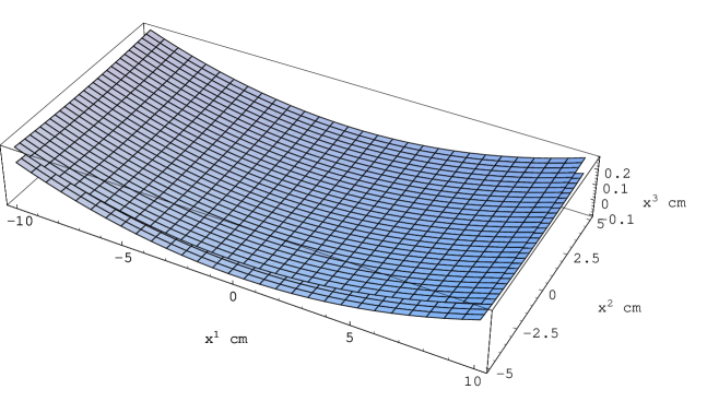
FIG. 1.: Curved Bragg mirror.

and Fig.2 shows the average radius of curvature of reflecting external surface of this plate.

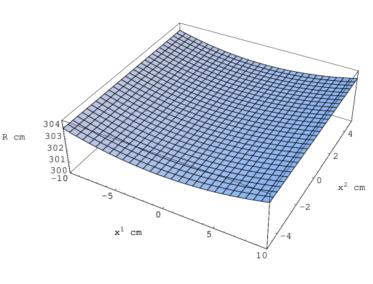
FIG. 2.: The mirror average curvature radius

As Fig.2 shows, the bent silicon plate average radius of curvature with such choice of parameters depends on the co-ordinates of a point on the reflecting surface and is being the value about $\displaystyle 3\times 10^{2}cm$. Let us discuss the most simple situation: the absorption of X-ray quanta passing through the deformed silicon plate (Bugger law).For this situation from equations (102) we obtain (from equations (102))

$\displaystyle\displaystyle\left[2i\frac{1}{k}n_{i}^{({\bf 0})}({\bf\xi})g^{ij}({\bf\xi}){\displaystyle{\frac{\partial}{\partial\xi^{j}}}}+\chi_{({\bf 0})}(\omega)\right]{\bf E}_{{\bf 0}}({\bf\xi},\omega)=0,$

for the simplicity we will neglect the dependence on Debye-Waller factor on the co-ordinates and from Takagi -Taupin equations (108)

$\displaystyle\displaystyle\left[2i\frac{1}{k}n_{i}^{({\bf 0})}\delta^{ij}{\displaystyle{\frac{\partial}{\partial\xi^{j}}}}+\chi_{({\bf 0})}(\omega)\right]E_{{\bf 0}}({\bf\xi},\omega)=0.$

Then solving the first equation by the characteristics method, i.e. by solving the system of the ordinary differential equations $\displaystyle{\displaystyle{\frac{d\xi^{j}(s)}{ds}}}=n_{i}^{({\bf 0})}({\bf\xi})g^{ij}({\bf\xi})$ with the initial conditions $\displaystyle\xi^{1}(0)=\xi_{0}^{1},\xi^{2}(0)=\xi_{0}^{2},$ $\displaystyle\xi^{3}(0)=0$, where $\displaystyle(\xi_{0}^{1},\xi_{0}^{2},0)$ are the entrance co-ordinates of the X-ray beam incident on the crystal, we obtain the following equation for transition function:

$\displaystyle\displaystyle T(\xi_{0}^{1},\xi_{0}^{2},h)=e^{-k\mathop{\rm Im}(\chi_{({\bf 0})}(\omega))s(\xi_{0}^{1},\xi_{0}^{2},h)},$

where $\displaystyle h$ is the perfect crystal length. The X-ray quanta optical path $\displaystyle s(\xi_{0}^{1},\xi_{0}^{2},h)$ in the deformed crystal can be obtained by solving the equation $\displaystyle\xi^{3}(s,\xi_{0}^{1},\xi_{0}^{2})=h$, where $\displaystyle\xi^{3}(s,\xi_{0}^{1},\xi_{0}^{2})$ is the solution of the ordinary differential equations system mentioned above. For the second equation, the solution i.e. the gating function can be easily obtained and does not differ from the perfect crystal plane-parallel plate at all.

$\displaystyle\displaystyle T=e^{-k\mathop{\rm Im}(\chi_{({\bf 0})}(\omega))\frac{h}{\sin(\theta)}},$

where $\displaystyle\theta$ is the angle between the X-ray quanta incident on the crystal and the normal to the perfect crystal entrance plane directed inside the crystal. Fig.3 show these transition functions for $\displaystyle\theta=\frac{\pi}{18},\varphi=\frac{\pi}{4},$ $\displaystyle h=0.01cm$ and quanta energies $\displaystyle 15KeV$.

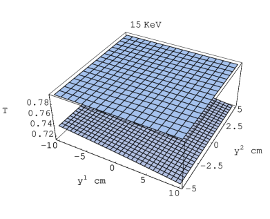
FIG. 3.: The silicon plate gating function. Here $\displaystyle y^{1}=\xi^{1}$ and $\displaystyle y^{2}=\xi^{2}$.

At the upper surface of this figure is presented the transition function for the plane-parallel perfect silicon crystal plate and the lower surface describes the X-ray quanta absorption by the deformed crystal. The distinction shows itself in the term of the second order and is very sufficient for such a thin plate. It means that even in such a simple situation as the absorption of X-ray quanta passing through the deformed crystal, the Takagi -Taupin equations don’t correctly describe the real experimental situation (this distinction can be neglected only for the crystal deformation with the average radius of curvature more then $\displaystyle 40m$).

To finally define the application range of Takagi -Taupin equations let us compare two terms:

1) $\displaystyle 1-[\sqrt{1+\alpha}n_{i}^{({\bf l})}+n_{\mu}^{({\bf 0})}\frac{\partial u^{\mu}({\bf\xi})}{\partial\xi^{i}}]g^{lj}[\sqrt{1+\alpha}n_{j}^{({\bf l})}+n_{\mu}^{({\bf 0})}\frac{\partial u^{\mu}({\bf\xi})}{\partial\xi^{j}}]$ in the second equation of the equation system (102) and

2) $\displaystyle\frac{1}{k}n_{i}^{({\bf l})}\delta^{ij}\tau_{\mu}{\displaystyle{\frac{\partial u^{\nu}({\bf\xi})}{\partial\xi^{j}}}}-\alpha$  in the second equation of the Takagi -Taupin equations system ( 108). Figure 4 shows the difference

$\displaystyle\displaystyle D=1+\alpha-[\sqrt{1+\alpha}n_{i}^{({\bf l})}+n_{\mu}^{({\bf 0})}\frac{\partial u^{\mu}({\bf\xi})}{\partial\xi^{i}}]g^{lj}[\sqrt{1+\alpha}n_{j}^{({\bf l})}+n_{\mu}^{({\bf 0})}\frac{\partial u^{\mu}({\bf\xi})}{\partial\xi^{j}}]-\frac{1}{k}n_{i}^{({\bf l})}\delta^{ij}\tau_{\mu}{\displaystyle{\frac{\partial u^{\nu}({\bf\xi})}{\partial\xi^{j}}}}$

between these values for the deformed silicon plate shown on the Fig.4-6 for the energies $\displaystyle 5KeV,10KeV$ and $\displaystyle 15KeV$ of the quanta.

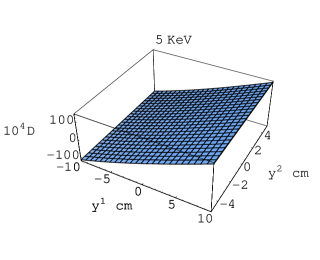
FIG. 4.: The value $\displaystyle D$ for the quanta with energy $\displaystyle 5KeV$ . Here $\displaystyle y^{1}=\xi^{1}$ and $\displaystyle y^{2}=\xi^{2}$.

FIG. 5.: The value $\displaystyle D$ for the quanta with energy $\displaystyle 10KeV$. Here $\displaystyle y^{1}=\xi^{1}$ and $\displaystyle y^{2}=\xi^{2}$.

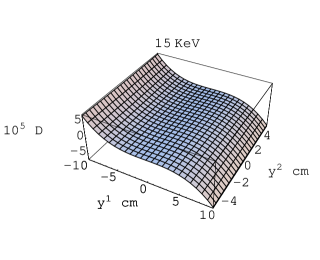
FIG. 6.: The value $\displaystyle D$ for the quanta with energy $\displaystyle 15KeV$. Here $\displaystyle y^{1}=\xi^{1}$ and $\displaystyle y^{2}=\xi^{2}$.

If one notify that for energies $\displaystyle 5KeV,10KeV$ and $\displaystyle 15KeV$ we have $\displaystyle\mathop{\rm Re}(\chi_{({\bf 0})}(\omega))=-0.394922\times 10^{-4}$,$\displaystyle-0.976232\times 10^{-5}$ and $\displaystyle\ -0.431670\times 10^{-5}$ accordingly, this figure shows that by accepting the simplifying assumptions in the equations (102) leading to the Takagi -Taupin equations we reject the values that are 10 times greater than the values we keep (for the crystals with the average radius of curvature less than $\displaystyle 10m$) while obtaining these equations. This difference shown in Fig.4 becomes less then $\displaystyle\mathop{\rm Re}(\chi_{({\bf 0})}(\omega))$ for the deformations with the curvature average radius more then $\displaystyle 40m$, i.e. very slightly deformed crystals. That is why one should use exactly the equations system (102) for the theoretical analysis. This system is a little bit more complicated but is suitable for the description of the X-ray optics devices being met with in practice.

VI           Bend Bragg mirror.

The equations (102) ( equations for the slowly varying amplitudes of the field of X-ray quanta in the two-wave dynamic diffraction on the deformed crystals) for the arbitrary deformation field can be solved in general only numerically. In the article we underlined more than once that the X-ray optics can be considered as the geometrical optics from the point of view of general electrodynamics. That is why to obtain the coefficient of Bragg reflection from the distorted Bragg mirror we will use the geometrical optics locality principle (see for ex. [17]) that evidently was first time introduced in electrodynamics by V.A. Fock [18] who investigated the reflection of the electromagnetic wave with smooth arbitrary shape front on the smooth arbitrary shaped surface. According to the locality principle the wave reflection in the every mirror point acts like if the incident wave is being smooth one and the curvilinear surface in this point is replaced by the tangent plane. But it is necessary to take into account that the incident and the reflection angle change their values from point to point on this surface. Consequently the locality principle allows us to use the reflection coefficients obtained for the plane waves and plane surfaces, and in particular the Bragg reflection coefficient for the diffraction X-ray optics as the primary approximation. The Bragg reflection coefficient in the case of the plane wave reflecting from the parallel-sided perfect crystal thick plate is determined by formula:

$${\cal R}=\frac{C\chi_{({\bf-l})}(\omega)}{\chi_{({\bf 0})}(\omega)(1+\beta)-{\displaystyle{\frac{\alpha}{2}}}\pm\sqrt{\left({\displaystyle{\frac{\chi_{({\bf 0})}(\omega)}{2}}}(1+\beta)-{\displaystyle{\frac{\alpha}{2}}}\right)^{2}-C^{2}\beta\chi^{2}(\omega)}}$$ (115)

where $\displaystyle C$ is the polarization factor mentioned above, $\displaystyle\beta=-{\displaystyle{\frac{n_{3}^{({\bf l})}}{n_{3}^{({\bf 0})}}}}$ is the asymmetry parameter, $\displaystyle\chi^{2}(\omega)=\chi_{({\bf-l})}(\omega)\chi_{({\bf l})}(\omega)$, $\displaystyle\alpha={\displaystyle{\frac{({\bf k}+{\bf\tau})^{2}-k^{2}}{k^{2}}}}$ is the parameter of precise Bragg condition deviation.

Let the X-ray quanta wave packet incident on the Bragg mirror with arbitrary smooth deformation field $\displaystyle{\bf u}({\bf\xi})$ has the electric vector for quanta with frequency $\displaystyle\omega$ ( or the energy $\displaystyle\varepsilon$ ) determined in the Lagrange co-ordinates system by the equation

$\displaystyle\displaystyle{\bf E}({\bf\xi},\omega)={\bf E}^{(0)}({\bf\xi},\omega)e^{ik(n_{i}^{(0)}\xi^{i}+n_{i}^{(0)}u^{i}({\bf\xi})+\Psi_{0}({\bf\xi},\varepsilon))},$

where $\displaystyle n_{i}^{(0)}$ are wave vector guiding cosines and $\displaystyle{\bf E}^{(0)}({\bf\xi},\omega)$ and $\displaystyle\Psi_{0}({\bf\xi},\varepsilon)$ are the slowly changing amplitude and phase of the X-ray quanta incident on the mirror. Then according to the locality principle of geometrical optics this reflection coefficient of the wave packet for distorted Bragg mirror has the functional form like that for the plane wave and plane mirror. But it is necessary to take into account that the values $\displaystyle\chi_{({\bf 0,\pm l})},C,\beta$  and $\displaystyle\alpha$ for the distorted Bragg mirror change from point to point on this mirror surface. If the dependence $\displaystyle\chi_{({\bf 0,\pm l})}$ on co-ordinates is determined by formula (89), the dependencies of $\displaystyle C$,$\displaystyle\beta$  and $\displaystyle\alpha$ on the co-ordinates can be defined by the following ideas. The wave covector components of the X-quanta incident on the distorted Bragg mirror in the Lagrange co-ordinate system to be determined by the equation

$\displaystyle\displaystyle k_{i}(\xi^{1},\xi^{2})=k\left[n_{i}^{({\bf 0})}+n_{\mu}^{({\bf 0})}\left(\frac{\partial u^{\mu}({\bf\xi})}{\partial\xi^{i}}\right)_{\xi^{3}=0}+\left(\frac{\partial\Psi_{0}({\bf\xi},\varepsilon)}{\partial\xi^{i}}\right)_{\xi^{3}=0}\right].$

Then the wave covector X-ray quanta components in the Lagrange co-ordinates system having diffracted on this mirror are determined by formula

$\displaystyle\displaystyle k_{i}(\xi^{1},\xi^{2})+\tau_{i}=k\left[\sqrt{1+\alpha}n_{i}^{({\bf l})}+n_{\mu}^{({\bf 0})}\left(\frac{\partial u^{\mu}({\bf\xi})}{\partial\xi^{i}}\right)_{\xi^{3}=0}+\left(\frac{\partial\Psi_{0}({\bf\xi},\varepsilon)}{\partial\xi^{i}}\right)_{\xi^{3}=0}\right].$

According to the definition we have for parameters $\displaystyle\alpha(\xi^{1},\xi^{2}),\beta(\xi^{1},\xi^{2})$ and $\displaystyle C(\xi^{1},\xi^{2})$

$$\displaystyle\alpha(\xi^{1},\xi^{2})=$$ (116)

$$\displaystyle\frac{2k\tau_{i}g^{ij}(\xi^{1},\xi^{2})n_{j}^{({\bf 0})}(\xi^{1},\xi^{2})+2k\tau_{i}g^{ij}(\xi^{1},\xi^{2})\left(\frac{\partial\Psi_{0}({\bf\xi},\varepsilon)}{\partial\xi^{j}}\right)_{\xi^{3}=0}+\tau_{i}g^{ij}(\xi^{1},\xi^{2})\tau_{j}}{k^{2}\left[1+2n_{i}^{({\bf 0})}(\xi^{1},\xi^{2})g^{ij}(\xi^{1},\xi^{2})\left(\frac{\partial\Psi_{0}({\bf\xi},\varepsilon)}{\partial\xi^{j}}\right)_{\xi^{3}=0}+\left(\frac{\partial\Psi_{0}({\bf\xi},\varepsilon)}{\partial\xi^{i}}\right)_{\xi^{3}=0}g^{ij}(\xi^{1},\xi^{2})\left(\frac{\partial\Psi_{0}({\bf\xi},\varepsilon)}{\partial\xi^{j}}\right)_{\xi^{3}=0}\right]};$$ (117)

$$\displaystyle\beta(\xi^{1},\xi^{2})=-\frac{n_{3}^{({\bf l})}(\xi^{1},\xi^{2})}{n_{3}^{({\bf 0})}(\xi^{1},\xi^{2})};$$ (118)

$$\displaystyle C(\xi^{1},\xi^{2})=n_{i}^{({\bf 0})}(\xi^{1},\xi^{2})g^{ij}(\xi^{1},\xi^{2})n_{j}^{({\bf l})}(\xi^{1},\xi^{2}),$$ (119)

where $\displaystyle n_{i}^{({\bf 0})}(\xi^{1},\xi^{2})$ and $\displaystyle n_{j}^{({\bf l})}(\xi^{1},\xi^{2})$ are the wave covectors guiding cosines of X-ray quanta falling and diffracted on the distorted Bragg mirror surface in the Lagrange co-ordinates system:

$$\displaystyle n_{i}^{({\bf 0})}(\xi^{1},\xi^{2})=n_{\mu}^{({\bf 0})}\left[\delta_{i}^{\mu}+\left(\frac{\partial u^{\mu}({\bf\xi})}{\partial\xi^{i}}\right)_{\xi^{3}=0}\right];$$ (120)

$$\displaystyle n_{i}^{({\bf l})}(\xi^{1},\xi^{2})=\frac{\left[\sqrt{1+\alpha}n_{i}^{({\bf l})}+n_{\mu}^{({\bf 0})}\left(\frac{\partial u^{\mu}({\bf\xi})}{\partial\xi^{i}}\right)_{\xi^{3}=0}+\left(\frac{\partial\Psi_{0}({\bf\xi},\varepsilon)}{\partial\xi^{i}}\right)_{\xi^{3}=0}\right]}{l(\xi^{1},\xi^{2})},$$ (121)

$$\displaystyle l(\xi^{1},\xi^{2})=\sqrt{\left[\sqrt{1+\alpha}n_{i}^{({\bf l})}+n_{\mu}^{({\bf 0})}\left(\frac{\partial u^{\mu}({\bf\xi})}{\partial\xi^{i}}\right)_{\xi^{3}=0}+\left(\frac{\partial\Psi_{0}({\bf\xi},\varepsilon)}{\partial\xi^{i}}\right)_{\xi^{3}=0}\right]g^{ij}(\xi^{1},\xi^{2})}$$ (122)

$$\displaystyle\times\sqrt{\left[\sqrt{1+\alpha}n_{j}^{({\bf l})}+n_{\mu}^{({\bf 0})}\left(\frac{\partial u^{\mu}({\bf\xi})}{\partial\xi^{j}}\right)_{\xi^{3}=0}+\left(\frac{\partial\Psi_{0}({\bf\xi},\varepsilon)}{\partial\xi^{j}}\right)_{\xi^{3}=0}\right]}$$ (123)

Consequently the Bragg reflection coefficient of the distorted mirror in this approximation looks like

$$\displaystyle{\cal R}(\xi^{1},\xi^{2}) \displaystyle= \displaystyle\frac{C\chi_{({\bf-l})}(\xi^{1},\xi^{2};\omega)}{\chi_{({\bf 0})}(\xi^{1},\xi^{2};\omega)(1+\beta)-{\displaystyle{\frac{\alpha(\xi^{1},\xi^{2})}{2}}}\pm\Delta(\xi^{1},\xi^{2})}$$ (124)

$$\displaystyle\Delta(\xi^{1},\xi^{2}) \displaystyle= \displaystyle\sqrt{\left({\displaystyle{\frac{\chi_{({\bf 0})}(\xi^{1},\xi^{2};\omega)}{2}}}(1+\beta)-{\displaystyle{\frac{\alpha(\xi^{1},\xi^{2})}{2}}}\right)^{2}-C^{2}\beta\chi^{2}(\xi^{1},\xi^{2};\omega)}$$ (125)

Here $\displaystyle\chi_{({\bf 0,\pm l})}(\xi^{1},\xi^{2};\omega)=\left(\chi_{({\bf 0,\pm l})}({\bf\xi};\omega)\right)_{\xi^{3}=0},\chi^{2}(\xi^{1},\xi^{2};\omega)=\chi_{({\bf l})}(\xi^{1},\xi^{2};\omega)\chi_{({\bf-l})}(\xi^{1},\xi^{2};\omega)$. The asymmetry parameter $\displaystyle\beta$ and the polarization factor defined by formulas (119) can be considered the same as for the plane mirror in the first approximation. If besides we neglect the Debye-Waller dependency on the co-ordinates, the formula (125) for the Bragg coefficient is extremely simplified:

$$\displaystyle{\cal R}(\xi^{1},\xi^{2})=$$ (126)

$$\displaystyle= \displaystyle\frac{C\chi_{({\bf-l})}(\omega)}{\chi_{({\bf 0})}(\omega)(1+\beta)-{\displaystyle{\frac{\alpha(\xi^{1},\xi^{2})}{2}}}\pm\sqrt{\left({\displaystyle{\frac{\chi_{({\bf 0})}(\omega)}{2}}}(1+\beta)-{\displaystyle{\frac{\alpha(\xi^{1},\xi^{2})}{2}}}\right)^{2}-C^{2}\beta\chi^{2}(\omega)}}.$$ (127)

The fact, that the distorted Bragg mirror with rather big average radius of curvature can be represented as a set of plane Bragg mirrors turned relatively to each other, is widely used in X-ray optics systems designing. Nevertheless we haven’t found the formulas (125-127) introducing this representation (or their analogues) in other papers. The linear dimensions of the area participating in the forming of the diffracted field in the point $\displaystyle(\xi^{1},\xi^{2})$ on the crystal surface are about the X-ray quanta crystal absorption length $\displaystyle l_{abs}\thicksim 10^{-2}\div 10^{-3}cm$. If the deformation field in this area can be considered as the constant value, the formulas (125-127) are quite applicable.

Once the Bragg reflection coefficient is obtained, we can define the field of X-ray quanta diffracted on the distorted Bragg mirror reflecting surface

$$\displaystyle E_{\pi,\sigma}(\xi^{1},\xi^{2};\omega) \displaystyle= \displaystyle{\cal R}(\xi^{1},\xi^{2})E_{\pi,\sigma}^{(0)}(\xi^{1},\xi^{2};\omega)e^{ik\Phi_{({\bf l})}(\xi^{1},\xi^{2})};$$ (128)

$$\displaystyle\Phi_{({\bf l})}(\xi^{1},\xi^{2}) \displaystyle= \displaystyle\left[\sqrt{1+\alpha}n_{i}^{({\bf l})}+n_{i}^{(0)}u^{i}({\bf\xi})+\Psi_{0}({\bf\xi},\varepsilon)\right]$$ (129)

The equations (125-127) and (129) solve the problem of X-ray quanta two-wave dynamic diffraction on the elastically deformed crystal in the Bragg geometry, i.e. on the incurved Bragg mirror. The only problem remaining is the X-ray quanta propagation and focusing in vacuum (or in the air), i.e. the Hemholts equation solution.

$\displaystyle\displaystyle(\Delta+k^{2})E({\bf r},\omega)=0$

with the assumption that on the distorted Bragg mirror surface there is the X-ray quanta field $\displaystyle A^{(0)}({\bf r},\omega)e^{ikS_{0}({\bf r})}$ defined with the amplitude  $\displaystyle A^{(0)}({\bf r},\omega)={\cal R}(\xi^{1},\xi^{2})E^{(0)}(\xi^{1},\xi^{2};\omega)$ and phase $\displaystyle S_{0}({\bf r},\varepsilon)=\Phi_{({\bf l})}(\xi^{1},\xi^{2},\varepsilon)$. Beyond the caustics this task can be solved by geometrical optics methods [17] leading to the formula

$$E({\bf r},\omega)={\cal R}(\xi^{1},\xi^{2})E^{0}(\xi^{1},\xi^{2};\omega)\sqrt{\frac{R_{1}R_{2}}{(S-R_{1})(S-R_{2})}}e^{ikS_{0}({\bf r})+ikS({\bf r},\xi^{1},\xi^{2})}$$ (130)

where

$$S({\bf r},\xi^{1},\xi^{2})=\sqrt{(x^{1}-\xi^{1}-u^{1}(\xi^{1},\xi^{2},0))^{2}+(x^{2}-\xi^{2}-u^{2}(\xi^{1},\xi^{2},0))^{2}+(x^{3}-u^{3}(\xi^{1},\xi^{2},0))^{2}}$$ (131)

is the distance from the Bragg mirror surface point with parameters $\displaystyle(\xi^{1},\xi^{2})$ to the point with co-ordinates $\displaystyle(x^{1},x^{2},x^{3})$, and $\displaystyle R_{1}$ and $\displaystyle R_{2}$ are the curvature radiuses of the wave diffracted on the Bragg mirror surface defined by the equations

$$\displaystyle R_{1,2} \displaystyle= \displaystyle\frac{-b\pm\sqrt{b^{2}-4ac}}{2a};$$ (132)

$$\displaystyle a \displaystyle= \displaystyle\delta^{ijl}N_{i}(\xi^{1},\xi^{2})\frac{\partial N_{j}(\xi^{1},\xi^{2})}{\partial\xi^{1}}\frac{\partial N_{l}(\xi^{1},\xi^{2})}{\partial\xi^{2}};$$ (133)

$$\displaystyle b \displaystyle= \displaystyle\delta^{ijl}N_{i}(\xi^{1},\xi^{2})\frac{\partial N_{j}(\xi^{1},\xi^{2})}{\partial\xi^{1}}\left(\frac{\partial x_{l}({\bf\xi})}{\partial\xi^{2}}\right)_{\xi^{3}=0}-\delta^{ijl}N_{i}(\xi^{1},\xi^{2})\frac{\partial N_{j}(\xi^{1},\xi^{2})}{\partial\xi^{2}}\left(\frac{\partial x_{l}({\bf\xi})}{\partial\xi^{1}}\right)_{\xi^{3}=0};$$ (134)

$$\displaystyle c \displaystyle= \displaystyle\delta^{ijl}N_{i}(\xi^{1},\xi^{2})\left(\frac{\partial x_{j}({\bf\xi})}{\partial\xi^{1}}\right)_{\xi^{3}=0}\left(\frac{\partial x_{l}({\bf\xi})}{\partial\xi^{2}}\right)_{\xi^{3}=0}.$$ (135)

Here $\displaystyle\delta^{ijl}$ is the fully asymmetrical tensor of the third rank ($\displaystyle\delta^{123}=1$), $\displaystyle N_{i}(\xi^{1},\xi^{2})$ is the normal vector to the X-ray quanta wave front on the Bragg mirror surface in the Euler co-ordinates system defined by the formula

$$\displaystyle N_{j}(\xi^{1},\xi^{2})=\frac{\left(\hat{J}^{-1}(\xi^{1},\xi^{2})\right)_{j}^{i}\left[\sqrt{1+\alpha}n_{i}^{({\bf l})}+n_{\mu}^{({\bf 0})}\left(\frac{\partial u^{\mu}({\bf\xi})}{\partial\xi^{i}}\right)_{\xi^{3}=0}+\left(\frac{\partial\Psi_{0}({\bf\xi},\varepsilon)}{\partial\xi^{i}}\right)_{\xi^{3}=0}\right]}{L(\xi^{1},\xi^{2})};$$ (136)

$$\displaystyle\left(L(\xi^{1},\xi^{2})\right)^{2}=\left(\hat{J}^{-1}(\xi^{1},\xi^{2})\right)_{j}^{i}\left[\sqrt{1+\alpha}n_{i}^{({\bf l})}+n_{\mu}^{({\bf 0})}\left(\frac{\partial u^{\mu}({\bf\xi})}{\partial\xi^{i}}\right)_{\xi^{3}=0}+\left(\frac{\partial\Psi_{0}({\bf\xi},\varepsilon)}{\partial\xi^{i}}\right)_{\xi^{3}=0}\right]$$ (137)

$$\displaystyle\times\delta^{jh}\left(\hat{J}^{-1}(\xi^{1},\xi^{2})\right)_{h}^{l}\left[\sqrt{1+\alpha}n_{l}^{({\bf l})}+n_{\mu}^{({\bf 0})}\left(\frac{\partial u^{\mu}({\bf\xi})}{\partial\xi^{l}}\right)_{\xi^{3}=0}+\left(\frac{\partial\Psi_{0}({\bf\xi},\varepsilon)}{\partial\xi^{l}}\right)_{\xi^{3}=0}\right]$$ (138)

where $\displaystyle\hat{J}^{-1}(\xi^{1},\xi^{2})$ is the matrix inverse to the Jacob matrix $\displaystyle\hat{J}(\xi^{1},\xi^{2})=\left\|\delta_{j}^{i}+{\displaystyle{\frac{\partial u^{i}({\bf\xi})}{\partial\xi^{j}}}}\right\|_{\xi^{3}=0}$  and $\displaystyle x_{l}({\bf\xi)=\xi}^{l}+u^{l}({\bf\xi})$ are the Euler co-ordinates of the deformed crystal points.

In the points where the equations $\displaystyle S=R_{1,2}$ are fulfilled, the geometric-optical solution (40) turns into the infinity (has a singularity). These points are called the focal ones and the set of the focal points is called the caustic. Consequently the multitude called the caustic is determined by the equations

$$x_{(f)1,2}^{j}=\left(\xi^{j}+u^{j}({\bf\xi})\right)_{\xi^{3}=0}+R_{1,2}(\xi^{1},\xi^{2})\delta^{ji}N_{i}(\xi^{1},\xi^{2})$$ (139)

As the example illustrating formulas (125)-(139) we will consider a simple situation when the plane waves packet of X-ray quanta with parallel vectors and energies in the interval from $\displaystyle 11KeV$ to $\displaystyle 17KeV$ incident on the plane-parallel silicon plate with thickness $\displaystyle h=0.1cm$ and reflection vector $\displaystyle{\bf\tau}(1,1,1)$ perpendicular to the plate entrance surface. We will consider the crystal plate oriented in such the way that the Bragg condition precisely holds for the X-ray quanta with energies $\displaystyle 15KeV$. Next this plate is distorted by momentums $\displaystyle M_{1}$ and $\displaystyle M_{2}$ uniformly distributed over the plate sides in such a way that the deformations field is determined by the formulas (114) from the previous part and the distorted Bragg mirror is the result of this deformation shown on Fig.1. Since by accepted condition the packet of plane waves is incident on this mirror, one would let $\displaystyle\Psi_{0}({\bf\xi},\varepsilon)=0$ in formulas (125)-(139) in this situation. The angle between the diffraction plate and the co-ordinate plate $\displaystyle(\xi^{1},\xi^{3})$ will be denoted as $\displaystyle\varphi$. Fig.7-10 shows the graphs obtained with the help of formula (127) for the module of coefficient of Bragg reflection from this distorted mirror for X-ray quanta energies $\displaystyle 11KeV,$ $\displaystyle 13KeV,$ $\displaystyle 15KeV$ and $\displaystyle 17KeV$ with $\displaystyle\varphi=0$.

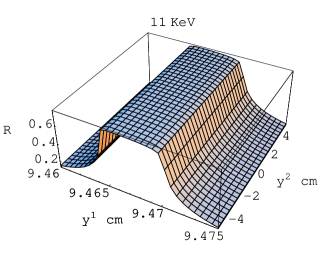
FIG. 7.: Bragg reflection coefficient. Here $\displaystyle y^{1}=\xi^{1}$ and $\displaystyle y^{2}=\xi^{2}$.

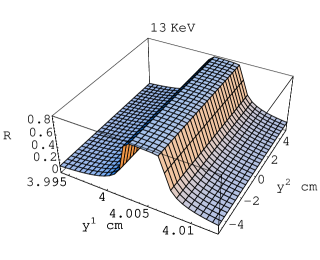
FIG. 8.: Bragg reflection coefficient. Here $\displaystyle y^{1}=\xi^{1}$ and $\displaystyle y^{2}=\xi^{2}$.

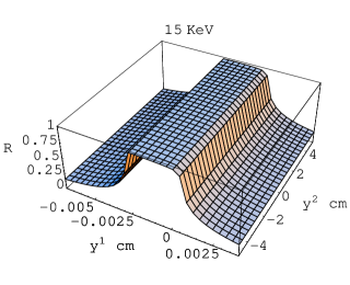
FIG. 9.: Bragg reflection coefficient. Here $\displaystyle y^{1}=\xi^{1}$ and $\displaystyle y^{2}=\xi^{2}$.

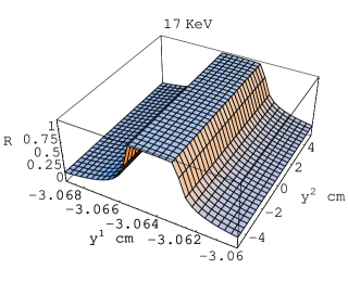
FIG. 10.: Bragg reflection coefficient. Here $\displaystyle y^{1}=\xi^{1}$ and $\displaystyle y^{2}=\xi^{2}$.

We remind that the caustics (the focal point multitude) of X-ray quanta diffracted on the Bragg mirror is defined exclusively by the X-ray radiation field and does not depend on the reflected quanta intensity distribution (Bragg radiation coefficient) on the crystal surface. By Fig.11-14 we give the caustics for X-ray quanta energies $\displaystyle 11KeV$, $\displaystyle 13KeV$, $\displaystyle 15KeV$ and $\displaystyle 17KeV$ obtained from formulas (138-139) for the whole Bragg mirror (without accounting the intensity distribution of quanta reflected on the whole surface of the mirror, i.e. without accounting the Bragg reflection coefficient dependency on the co-ordinates of the point on the mirror surface).

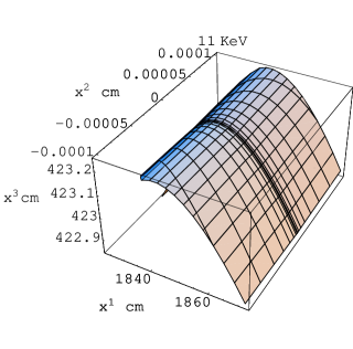
FIG. 11.: Diffracted quanta caustic.

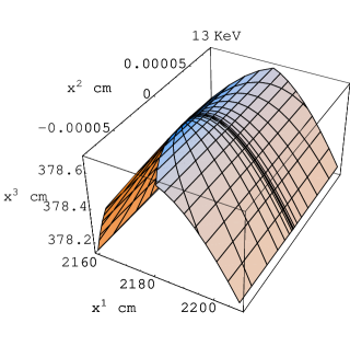
FIG. 12.: Diffracted quanta caustic.

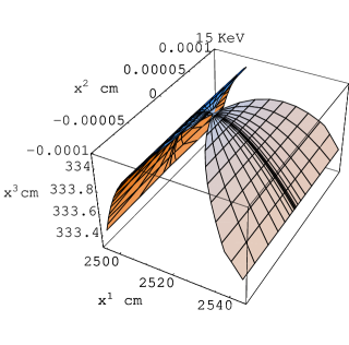
FIG. 13.: Diffracted quanta caustic.

FIG. 14.: Diffracted quanta caustic.

It is clear that in experiment there will be presented only the part of this caustic surface which X-ray quanta are coming at, once reflected from the mirror area with the Bragg reflection coefficient sufficiently differing from null. These areas for our example are shown on fig.5. Fig.15-18 shows caustics (focal points manifold) obtained also with the help of formulas ( 135-139) but taking into account the dependency of Bragg reflection coefficients on the co-ordinates.

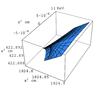
FIG. 15.: Caustic at $\displaystyle 9.46\leq\xi^{1}\leq 9.475$.

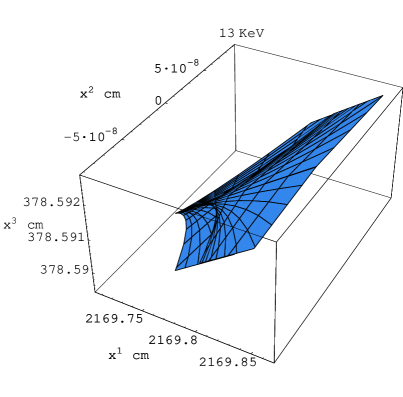
FIG. 16.: Caustic at $\displaystyle 3.994\leq\xi^{1}\leq 4.013$.

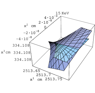
FIG. 17.: Caustic at $\displaystyle-0.007\leq\xi^{1}\leq 0.004$.

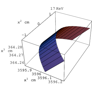
FIG. 18.: Caustic at $\displaystyle-3.069\leq\xi^{1}\leq-3.06$.

It is worth mentioning that even in the simplest case we deal with rather complicated (that is clear from these diagrams) combination of elementary differentiable peculiarities (catastrophes) $\displaystyle A_{1},A_{2},A_{3},A_{4}$ and $\displaystyle D_{4}^{\pm}$ (by V.I. Arnold classification) of phase function $\displaystyle\Phi_{({\bf l})}(\xi^{1},\xi^{2},\varepsilon)+S({\bf r},\xi^{1},\xi^{2})$. That is why one can not even talk about the fit (frequently met in the X-ray optics articles, see for ex. [21]) of X-ray quanta intensity distribution near the caustics (focus) with Gaussian function [20] . The caustics intensity distribution is described by special catastrophes functions the simplest of them being Airy functions and Piersey integral [22] investigated in details in articles [23]. If one models the intensity distribution by Gaussian beams, it is necessary to use the special method of Gaussian beams summing discussed in [24].

VII Acknowledgments

We are indebted to Prof. S. Maksimenko and Prof. G. Slepyan for stimulating discussions.