Atomic collision dynamics in optical lattices

Abstract

We simulate collisions between two atoms, which move in an optical lattice under the dipole-dipole interaction. The model describes simultaneously the two basic dynamical processes, namely the Sisyphus cooling of single atoms, and the light-induced inelastic collisions between them. We consider the $J=1/2\rightarrow J=3/2$ laser cooling transition for Cs, Rb and Na. We find that the hotter atoms in a thermal sample are selectively lost or heated by the collisions, which modifies the steady state distribution of atomic velocities, reminiscent of the evaporative cooling process.

I Introduction

Laser cooling and trapping techniques have made it possible to study and manipulate samples of cold neutral atoms [1]. It has lead to the precision control of atomic matter, and also opened new possibilities for investigations of interaction dynamics between atoms, especially those mediated by light [2]. By controlling the internal states of the atoms we obtain access to their center-of-mass motion [1, 3]. Sisyphus cooling and polarization gradient cooling methods [4], which allow one to break the Doppler limit for low temperatures, are based on the way polarized light connects to the atomic states. By combining more than one laser beam we can introduce a spatially changing polarization state into the total light field interacting with atoms. As light introduces Stark shifts on atomic states, the spatially changing polarization appears as a spatially changing potential for atoms with a suitable angular momentum state structure. In addition to the cooling effect, this has made it possible to build periodic or quasiperiodic lattices [5], where the light field traps the atoms. We describe the Sisyphus cooling and lattice structure in Sec. II.

The basic laser cooling method is Doppler cooling [1], which is produced by the random scattering of photons absorbed from the laser beam. This cooling mechanism is not related to the polarization states of light. For alkali atoms this method has a limiting temperature, the Doppler temperature $T_{D}=\hbar\Gamma/2k_{B}$, where $\Gamma$ is the atomic linewidth. Using the polarization states, i.e., Sisyphus cooling and polarization gradient cooling, one can go below $T_{D}$ until the photon recoil limit, $T_{R}$, is reached, and creating a lattice as a byproduct. The values of $T_{R}$ and $T_{D}$ for used elements are given in Table I. Typically one reaches a thermal equilibrium where the atoms are more or less localized at lattice sites, but can also move between them. The efficiency and the degree of localization have been studied thoroughly in the past [5]. Since the best filling ratios (number of atoms per site) with small-detuning lattices are on the order of 10 % [5], one can consider the gas sample as noninteracting. Larger filling ratios have been achieved lately by special techniques in far-detuned optical lattices [6]. Based on the experience in standard magneto–optical traps (MOTs), the increasing density for small-detuning lattices is expected to lead to strong loss and heating of atoms due to collisions, which become strongly inelastic in the presence of the near-resonant cooling light [2, 7]. By a “small-detuning lattice” we mean one that is detuned a few atomic linewidths below the transition frequency.

The light-assisted collisions are based on the fact that the two slowly approaching atoms form a quasimolecule, which the light can excite resonantly during the approach, even though the cooling beams are clearly off the resonance with the atomic transition energy which corresponds only asymptotically to the molecular state transition energy. The resonance occurs at relatively long distances [8], where the dominant contribution to the molecular behavior, i.e., the interaction potential between atoms, comes from the dipole-dipole interaction (DDI). We describe these collisions in Sec. III, and derive an expression for DDI in Sec. IV. We have presented the first results of our work in a previous short publication [9], where details of the derivation were omitted, so here we present them in full. It should be noted that one can develop e.g. a mean field approach to atom-atom processes via the DDI [10, 11, 12, 13]. In our approach, albeit with some limitations, we allow the atoms to move. Furthermore, we consider the problem in the atom-atom basis, with the full Zeeman substate structure, in the presence of the cooling/lattice-building laser beams with spatially changing polarization structure. Thus our model treats the Sisyphus cooling and localization of the atoms, and the atomic collisions dynamics consistently, within the same framework.

In order to describe two multistate atoms moving quantum mechanically as wave packets in position and momentum space, and being coupled both to the spatially changing laser field as well as the vacuum field producing spontaneous emission, we would in principle have to use the density matrix description. This is not computationally possible currently, but we can go around the problem by describing the spontaneous emission with quantum jumps. As described in Sec. V, we use the Monte Carlo wave function (MCWF) method to build a statistical ensemble of time evolution histories, which approximates adequately the actual density matrix [14, 15, 16]. To implement this approach on our description of atomic collisions in lattices is not straightforward, and in Sec. VI we describe the details related to numerical simulations. Inelastic collisions in MOTs have been modelled extensively with semiclassical models [17]. We describe these models briefly in Sec. VII. They provide a tool for understanding some of the physics behind the numerical data, and for estimating the processes affecting the multitude of boundaries for the numerical methods.

Our Monte Carlo simulation results, presented in Sec. VIII, indicate that the hotter atoms in our thermal sample, due to their stronger mobility between the lattice sites, are more likely to collide inelastically than the colder ones. On the other hand, the simulations, supported by semiclassical estimates, show that inelasticity plays a relevant role only if the atoms end up in the same lattice site simultaneously. In other words, the effect of the dipole-dipole interaction remains small if the atoms do not share the same lattice site. This, of course, also depends on the chosen laser field parameters such as intensity and detuning. When the close, same-site encouter occurs, however, it is most likely a strongly inelastic one leading to the loss of atoms. Basically, we see a process similar to evaporative cooling, where the hotter atoms are selectively heated or ejected from the lattice. It should be noted, though, that despite the fully quantum mechanical nature of our approach, it still omits many other effects affecting the atomic cloud in the lattice. Photons scattered incoherently by atoms can be reabsorbed, which produces a radiation pressure; this process also heats the atomic cloud as its density and thus optical thickness increases [1].

The observations made in this paper follow those from our previous study [9]. The results given in this paper, however, have been obtained with an improved approach compared to Ref. [9], and we have also extended our studies to all the basic alkali species. Furthermore, here we give the detailed description of our approach and its computational aspects. Finally, the discussion in Sec. IX concludes our presentation.

II Sisyphus cooling and optical lattices

In this Section we present the atom–laser system under study and describe briefly the basics of Sisyphus laser cooling of neutral atoms in an optical lattice. Detailed review of the subject can be found in Refs. [1, 4, 5].

A Atom–laser system

We consider here atoms having ground state angular momentum $J_{g}=1/2$ and excited state angular momentum $J_{e}=3/2$ corresponding to alkali metal elements when the hyperfine structure is neglected. The resonance frequency between the states is $\omega_{0}$ so that $\hbar\omega_{0}=E_{e}-E_{g}$ where $E_{e}$ and $E_{g}$ are energies of the ground and the excited states in zero field. A single atom has two ground state sublevels $|g_{\pm 1/2}>$ and four excited state sublevels $|e_{\pm 3/2}>$ and $|e_{\pm 1/2}>$ where the half–integer subscripts indicate the quantum number $m$ of the angular momentum along the $z$ direction, see Fig. 1. The values of atomic masses that are used in our simulations are those of cesium (¹³³Cs), rubidium (⁸⁵Rb) and sodium (²³Na) which are the conventional alkali metal elements used for laser cooling of neutral atoms, see Table I.

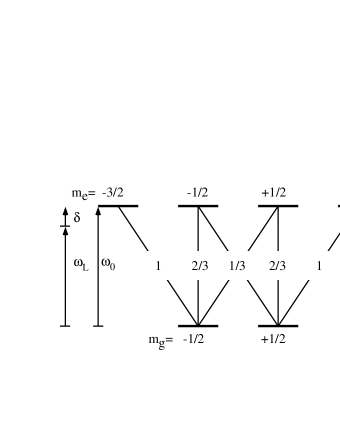
FIG. 1.: The level structure of a single atom. We show the squares of the Clebsch-Gordan coefficients of corresponding transitions describing the strengths of couplings between the Zeeman sublevels. The difference between the laser frequency $\omega_{L}$ and the atomic frequency $\omega_{0}$, i.e., the laser detuning, is $\delta$.

The laser field consists of two counter–propagating beams with orthogonal linear polarizations and with frequency $\omega_{L}$. The total field has a polarization gradient in one dimension and reads

$${\bf E}(z,t)={\cal E}_{0}({\bf e}_{x}e^{ik_{r}z}-i{\bf e}_{y}e^{-ik_{r}z})e^{-i\omega_{L}t}+c.c.,$$ (1)

where ${\cal E}_{0}$ is the amplitude and $k_{r}$ the wavenumber. With this field, the polarization changes from circular $\sigma^{-}$ to linear and back to circular in the opposite direction $\sigma^{+}$ when $z$ changes by $\lambda_{L}/4$ where $\lambda_{L}$ is the wavelength of the lasers.

The periodic polarization gradient of the laser field is reflected in the periodic light shifts, AC–Stark shifts, of the atomic sublevels creating the optical lattice structure. The relative strengths of the couplings between a single ground state sublevel and various excited state sublevels vary spatially according to the polarization of the light field due to unequal values of the Clebsch–Gordan coefficients for different transitions. This induces light shifts and produces a periodic optical potential structure such that the shape of the light-induced potentials is the same for the two ground state sublevels but the potentials are shifted spatially with respect to each other by $\lambda_{L}/4$, see Fig. 2. The top of the optical potential for one sublevel coincide with the bottom of the other one.

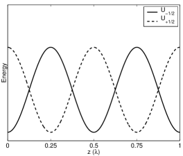
FIG. 2.: Schematic view of the optical potentials for the two ground state Zeeman sublevels. Lattice structure is created due to the periodic polarization gradient of the laser field.

B Sisyphus cooling

When the atomic motion occurs in a suitable velocity range, optical pumping of the atom between ground state sublevels reduces the kinetic energy of the atom [4]. This occurs because within the suitable velocity range, quantum jumps and optical pumping to another ground state sublevel tend to occur when the atom is near the top of the optical potential and is transferred to the bottom of the other one due to a quantum jump. Thus the subsequently emitted photon has a larger energy than the absorbed one and the kinetic energy of the atom is therefore reduced, and the atom is cooled. After several such cooling cycles the atom localizes into the optical potential well, i.e., into an optical lattice site. Figure 3 shows the optical pumping cycles between the ground state sublevels cooling an atom, and the oscillations of the atomic wave packet after localization into an optical lattice site.

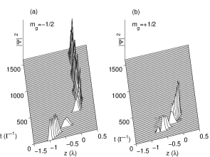
FIG. 3.: Sisyphus cooling and the localization of an atom into the optical lattice. We show a possible time evolution for a single atom wave packet for two ground state Zeeman levels, (a) $m_{g}=-1/2$, (b) $m_{g}=+1/2$. The result shows the optical pumping cycles and the localization of a single atom into the optical lattice. This example forms one member of a Monte Carlo simulation, and the discontinuous changes between the two ground states are due to quantum jump events from the excited state (not shown), selected to happen randomly with an appropriately weighted probability. If the run is repeated, the jumps would appear at different times again.

The intensity of the laser field and the strength of the coupling between the field and the atom is described by the Rabi frequency $\Omega=2d{\cal E}_{0}/\hbar$ where $d$ is the atomic dipole moment of the strongest transition between the ground and excited states. The detuning of the laser field from the atomic resonance is given by $\delta=\omega_{L}-\omega_{0}$. As a unit for $\Omega$ and $\delta$ we use the atomic linewidth $\Gamma$.

TABLE I.: Atomic properties. Masses $M$ in a.u. and linewidth energies $\epsilon=(\hbar\Gamma)/E_{r}$ (for the definition of the recoil unit $E_{r}$ see Table III). The Doppler temperature $T_{D}$ and the recoil temperature $T_{R}=\left(\hbar^{2}k_{r}^{2}\right)/Mk_{B}$ in $\mu K$. Here $k_{r}$ is the wavenumber of the laser.

property	Cs	Rb	Na
$M$	133	85	23
$\epsilon$	2400	1600	400
$T_{D}$	120	142	238
$T_{R}$	0.20	0.37	2.4

C Localization in lattice

When the steady state is reached after a certain period of cooling, atoms are to a large extent localized into the lattice sites. In this study we deal with near–resonant bright optical lattices where the laser field is detuned a few atomic linewidths to the red of the atomic transition. The laser parameters $\Omega$ and $\delta$ determine if the lattice is in the “jumping” or in the “oscillating” regime, depending on the average number of atomic oscillations in a single lattice site before the atom is optically pumped to neighboring sites [18]. It must be noted that tight localization and occupation of the lowest vibrational levels of a periodic lattice potential increases the optical pumping time $\tau_{p}$ and the time of localization within a single lattice site becomes longer compared to the semiclassical values presented in Table II.

We are interested in the effect of inelastic collisions between atoms in the presence of near–resonant light [2] in optical lattices. These collisions occur when two atoms occupy the same lattice site. To observe efficiently the effect of inelastic collisions we have chosen $\Omega$ and $\delta$ in most of the simulations so that the lattice is in the “jumping” regime, i.e., semiclassically speaking the atoms on average do not have time for a single full oscillation before optical pumping transfers them to a neighboring lattice site.

Steady state properties of the atomic cloud in the lattice are characterized e.g. by the average kinetic energy per atom, the spatial probability distribution or the momentum probability distribution. These are results which we obtain from our simulations. We keep the detuning fixed $(\delta=-3\Gamma)$ and vary the Rabi frequency $\Omega$, which gives various values for the optical potential modulation depth

$$U_{0}=-\frac{2}{3}\hbar\delta s_{0},$$ (2)

where $s_{0}$ is the saturation parameter given by

$$s_{0}=\frac{\Omega^{2}/2}{\delta^{2}+\Gamma^{2}/4}.$$ (3)

The spatially modulated optical potentials are

$$U_{-}=U_{0}\sin^{2}(k_{r}z),$$ (4)

$$U_{+}=U_{0}\cos^{2}(k_{r}z),$$ (5)

for ground states $m_{g}=-1/2$ and $m_{g}=+1/2$ respectively [18]. The parameters used in our simulations along with relevant lattice properties are summarized in Table II.

TABLE II.: Laser parameters used in the simulations and the corresponding lattice properties: Detuning $\delta$, Rabi frequency $\Omega$, lattice modulation depth $U_{0}$, semiclassical average number of oscillations in a lattice site $N_{osc}=\Omega_{osc}\tau_{p}$, and saturation parameter $s_{0}$. We use the semiclassical average oscillation frequency $\Omega_{osc}$ discussed in  [18]. Units are given in parenthesis and the simulations are labeled by the element and the lattice depth.

$\displaystyle{\Omega}(\Gamma)$	$\displaystyle{\delta}(\Gamma)$	$\displaystyle{U_{0}}(E_{r})$	$\displaystyle{N_{osc}}$	$\displaystyle{s_{0}}$	Simulation label
1.2	-3.0	374	0.93	0.08	Cs374
1.5	-3.0	584	0.74	0.12	Cs584
2.5	-3.0	1621	0.47	0.33	Cs1621
1.8	-3.0	560	0.76	0.18	Rb560
2.8	-3.0	339	0.98	0.42	Na339
3.5	-3.0	530	0.78	0.66	Na530

Collisions and radiative heating increase the relative velocity between the atoms [2]. This heats up the atoms and it is possible for a colliding pair to escape from the lattice. One can calculate semiclassically the critical momentum $p^{sc}_{c}$ giving the point in momentum ($p$) space where the cooling force has its maximum value [4]. In Section VI F below, we discuss for which values of the momentum $p_{c}$ we may neglect energetic histories and consider the corresponding atoms lost from the lattice.

III Binary interactions between cold atoms

In this Section we give a simple description of collisions between two cold atoms in the presence of near resonant light [2] and discuss the background of this phenomenon to occur in an optical lattice.

A Binary interactions

In this study, we consider atomic gases with an occupation density of $\rho_{o}=25$ %, i.e., every fourth lattice site is occupied and the average distance between two atoms is $z_{a}=\lambda$. For Cs this corresponds to a density of $1.62\times 10^{12}$ atoms/cm³. This atomic gas density is low enough that collisions can be treated as binary processes: i) The collision range is an order of magnitude smaller than $z_{a}$, and ii) for a Cs atomic mass, atoms with typical maximum velocities produced in our simulations need to have evolved over a time larger than $75\,\Gamma^{-1}$ to travel a distance $z_{a}$ and they scatter a large enough number of photons that there is negligible memory effects between two collision events. Thus, the binary collision picture is justified in our calculations.

Let us consider two atoms with a temperature around or below the Doppler temperature $T_{D}$. If such two atoms collide they form a quasimolecule which a near resonant light may excite when the atoms approach each other. This occurs at an internuclear distance called the Condon point $(r_{c})$ where the excited state electronic molecular potential becomes resonant with the ground state potential as displayed in Fig. 4.

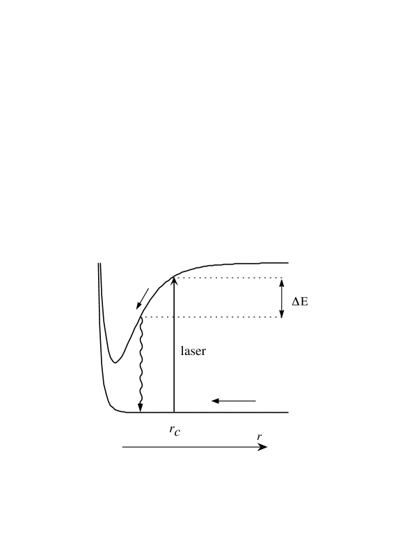
FIG. 4.: Radiative heating of colliding atoms. The quasimolecule is excited at the Condon point $r_{c}$ and accelerated on the upper level before spontaneous decay terminates the process.

We neglect the hyperfine structure of the atoms and do not consider the ground state hyperfine structure changing collisions, but concentrate on the effects based on radiative heating and escape of the colliding pair. In this process, the resonant excitation of a quasimolecule terminates in spontaneous decay and the colliding pair of atoms gains kinetic energy due to acceleration on an attractive molecular excited state before decay occurs, see Fig. 4. In principle it is also possible to loose atoms from the trap via fine structure changing collisions [2]. In this work, the loss fraction of fine structure changing collisions is assumed to be negligible compared to the radiative escape mechanism. The small detuning of the lasers makes $r_{c}$ very large, and the probability for surviving to the small internuclear distances required for the fine structure change is rather small. Furthermore, the energy increase caused by this mechanism is large and leads mainly to loss of atoms, contributing to heating only via secondary collisions. These secondary collisions are still rather rare in the low-density gas samples of laser cooled atoms.

An essential ingredient in the kinetic energy increasing collision process is the excitation of the large fraction of the population into the attractive excited state. The excited state population fraction in turn depends on the relative velocity between the interacting atoms when they reach $r_{c}$ for the attractive molecular states. For the collisions in the lattice, the relative velocity in turn depends on the optical lattice modulation depth. The deeper the lattice, the higher the relative velocity of the atoms when they end up in the same lattice site and collide. We consider here lattices with modulation depths in the range $339E_{r}\leq U_{0}\leq 1621E_{r}$, where $E_{r}$ is the recoil energy, cf. Table III. Thus, the relative velocities before a collision remain low, which keeps the excitation probability large. The small detuning keeps the excitation probability large also since the excited state slope decreases with the detuning; this increases the interaction time for moving atoms at the vicinity of the resonance point $r_{c}$.

B Collisions in lattices

Theoretical and experimental collision studies in MOTs show that the atomic cloud is heated by the radiative mechanism described above. Atoms may also escape from a MOT by this mechanism [2, 7]. Thus these collisions set a limit for atomic densities and temperatures of the cloud in a MOT when the density is increased so that binary interactions begin to have a clear effect. Typical densities achieved in MOTs are around $10^{11}$ atoms/cm³ and temperatures around or below the Doppler cooling limit [2].

Similar effects are expected in an optical lattice when the occupation density of the lattice increases. What is not directly expected is that there is a parameter region where a possible cooling process in a dense lattice occurs due to collisions. This is due to the fact that the colliding pair of atoms carry more kinetic energy than localized ones and during a collision they almost always gain sufficient energy to escape from the lattice. Thus those atoms that have not collided inelastically and remain in a lattice, have less kinetic energy per atom. Moreover, they can also thermalize via elastic ground-ground collisions. In our study, we neglect the rescattering of photons and consequently the total pattern of cooling and heating is not studied. Here we only consider the effects of collisions. The complete problem is simply not computationally tractable within our framework.

Atomic interactions in lattices are usually modelled assuming fixed positions for both atoms and calculating how the atomic energy levels are shifted by the interaction [10, 11, 12, 13]. These static models ignore the dynamical nature of the collision processes described here. When allowing the atoms to move the problem becomes complicated and computationally extremely tedious. To make numerically feasible calculations, we have fixed one atom and allow the other one to move freely, as described further in Sec. VI B.

IV Atomic basis formulation and dipole-dipole interaction

In this section we describe the two–atom product state basis [19] and the dipole–dipole interaction (DDI) between two atoms in our one-dimensional $(1D)$ study.

A Atomic basis formulation

We do not use the adiabatic elimination of the excited states, which is typically employed in order to simplify the equations for atomic motion [20]. By keeping the excited states in the calculation we are able to account for the dynamical nature of atomic interactions and the radiative heating/escape mechanism.

In general the product state basis vectors are:

$$|j_{1}{m_{1}}\rangle_{1}|j_{2}{m_{2}}\rangle_{2},$$ (6)

where $j_{1}$ and $j_{2}$ denote the ground or excited state (in our case $g$ for the ground state ${}^{2}S_{1/2}$, $e$ for the ²P_3/2 excited state) and $m_{1}$, $m_{2}$ denote the quantum number for the component of $j$ along the quantization axis $z$ for atom 1 and 2 respectively. The total number of states is $6\times 6=36$.

We have to fix the position of one atom, as described in Sec. VI B. If the position of atom 1 is fixed, the binary system wave function depends now only on the position of the moving atom 2

$$|\psi(z_{2},t)\rangle=\sum_{j_{1},j_{2},m_{1},m_{2}}\psi^{j_{1},m_{1}}_{j_{2},m_{2}}(z_{2},t)|j_{1}{m_{1}}\rangle_{1}|j_{2}{m_{2}}\rangle_{2}.$$ (7)

The atomic spatial dimensionality of the problem is reduced from two to one. The relative coordinate $z$ between atoms is now $z=z_{2}-z_{f}$ where $z_{f}$ is the position of the fixed atom, see Sec. VI B.

In the atomic product state basis [19], our system Hamiltonian is

$$H_{S}=H_{1}+H_{2}+V_{dip}.$$ (8)

Here, $V_{dip}$ includes the interaction between the atoms and $H_{1}=\widetilde{H}_{1}\otimes\openone_{2}$ and $H_{2}=\openone_{1}\otimes\widetilde{H}_{2}$, where the operators $\openone_{\alpha}$ are unity operators in atom $\alpha$ subspace, and the single atom Hamiltonian for atom $\alpha$ ($\alpha=1,2$) is, after the Rotating Wave Approximation (RWA),

$$\widetilde{H}_{\alpha}=\frac{p_{\alpha}^{2}}{2M}-\hbar\delta P_{e,\alpha}+\widetilde{V}_{\alpha}.$$ (9)

Here, $P_{e,\alpha}=\sum_{m=-3/2}^{3/2}|e_{m}\rangle_{\alpha}~{}_{\alpha}\langle e_{m}|$, and the interaction between a single atom $\alpha$ and the field is

$$\widetilde{V}_{\alpha} = -i\frac{\hbar\Omega}{\sqrt{2}}\sin(kz_{\alpha})\left\{|e_{3/2}\rangle_{\alpha}~{}_{\alpha}\langle g_{1/2}|\right.$$ (13)

$$+\frac{1}{\sqrt{3}}\left.|e_{1/2}\rangle_{\alpha}~{}_{\alpha}\langle g_{-1/2}|\right\}$$

$$+\frac{\hbar\Omega}{\sqrt{2}}\cos(kz_{\alpha})\left\{|e_{-3/2}\rangle_{\alpha}~{}_{\alpha}\langle g_{-1/2}|\right.$$

$$+\frac{1}{\sqrt{3}}\left.|e_{-1/2}\rangle_{\alpha}~{}_{\alpha}\langle g_{1/2}|\right\}+h.c.,$$

where $z_{\alpha}$ is the position operator of atom $\alpha$.

B Resonant dipole–dipole interaction

In order to get the DDI potential, $V_{dip}$, in Eq. (8), we have calculated the Master Equation for the atom and laser field in question, and identified the DDI. Our approach follows the lines of Appendix A in Ref. [21]. As it is beyond the scope of this paper to go through the derivation of the DDI potential in detail, we shall refer to equation (Ax) in Ref. [21] as Eq. (LMAx). We identify $V_{dip}$ as the terms similar to $\Delta_{11}$ and $\Delta_{22}$ with $\left<n_{\omega}+1\right>=1$ in Eq. (LMA21).

First, it is convenient to write the non-interacting system Hamiltonian $H_{1}+H_{2}$ in a basis of center-of-mass and relative coordinates:

$${\bf P}={\bf p}_{1}+{\bf p}_{2},\;\;\;{\bf p}=\frac{{\bf p}_{2}-{\bf p}_{1}}{2}.$$ (14)

With these coordinates, the interaction potential with the laser field, $V=\widetilde{V}_{1}\otimes\openone_{2}+\openone_{1}\otimes\widetilde{V}_{2}$, reads

$$V = -i\frac{\hbar\Omega}{\sqrt{2}}\sin(kZ)\cos\left(k\frac{z}{2}\right)\left(S_{+,+}^{1}\otimes\openone_{2}+\openone_{1}\otimes S_{+,+}^{2}\right)$$ (19)

$$+i\frac{\hbar\Omega}{\sqrt{2}}\cos(kZ)\sin\left(k\frac{z}{2}\right)\left(S_{+,+}^{1}\otimes\openone_{2}-\openone_{1}\otimes S_{+,+}^{2}\right)$$

$$+i\frac{\hbar\Omega}{\sqrt{2}}\cos(kZ)\cos\left(k\frac{z}{2}\right)\left(S_{+,-}^{1}\otimes\openone_{2}+\openone_{1}\otimes S_{+,-}^{2}\right)$$

$$+i\frac{\hbar\Omega}{\sqrt{2}}\sin(kZ)\sin\left(k\frac{z}{2}\right)\left(S_{+,-}^{1}\otimes\openone_{2}-\openone_{1}\otimes S_{+,-}^{2}\right)$$

$$+h.c.,$$

where $Z$ and $z$ are the center-of-mass and relative coordinates along the $z$-axis and

$$S_{+,q}^{\alpha}=\sum_{m=-1/2}^{m=1/2}CG_{m}^{q}|e_{m+q}\rangle_{\alpha}~{}_{\alpha}\langle g_{m}|.$$ (20)

Here $CG_{m}^{q}$ are the appropriate Clebsch-Gordan coefficients and $q$ is the polarization label in the spherical basis. We rewrite similarly the interaction with the vacuum electromagnetic field in terms of the relative coordinates (14). The DDI terms are identified after we have considered the damping part of $\dot{\rho}$ [cf. Eq. (LMA17)] in the derivation of the Master Equation for our two-atom system.

Following [21], we note that the DDI potential is found as

$$V_{dip} = -\frac{3}{8}\hbar\Gamma\frac{1}{\pi}\int_{0}^{\infty}d\omega\left(\frac{\omega}{\omega_{0}}\right)^{3}P\left(\frac{1}{\omega-\omega_{0}}\right)\times$$ (26)

$$\left\{j_{0}\left(\omega\frac{r}{c}\right)\left(\frac{1}{3}({\cal S}_{++}{\cal S}_{-+}+{\cal S}_{+-}{\cal S}_{--})-\frac{2}{3}{\cal S}_{+0}{\cal S}_{-0}\right)\right.$$

$$+j_{2}\left(\omega\frac{r}{c}\right)\left[P_{2}(\cos\theta_{r})\left(-\frac{2}{3}({\cal S}_{++}{\cal S}_{-+}+{\cal S}_{+-}{\cal S}_{--})\right.\right.$$

$$\left.+\frac{4}{3}{\cal S}_{+0}{\cal S}_{-0}\right)+\frac{1}{3\sqrt{2}}P_{2}^{1}(\cos\theta_{r})\cos\phi_{r}\times$$

$$\left(-{\cal S}_{++}{\cal S}_{-0}+{\cal S}_{+0}{\cal S}_{--}-{\cal S}_{+0}{\cal S}_{-+}+{\cal S}_{+-}{\cal S}_{-0}\right)$$

$$+\frac{1}{3}P_{2}^{2}(\cos\theta_{r})\cos 2\phi_{r}\left.\left.\left({\cal S}_{++}{\cal S}_{--}+{\cal S}_{+-}{\cal S}_{-+}\right)\frac{}{}\!\right]\right\},$$

where $P(x)$ is Cauchy’s principal value, $j_{\ell}$ are spherical Bessel functions of the first kind, $P_{2}$ is Legendre polynomial, and $P_{m}^{n}$ are associated Legendre functions. The angles $\theta_{r}$ and $\phi_{r}$ are the angles of the relative coordinate ${\bf r}$ in the spherical basis. We have also introduced the operators

$${\cal S}_{+q}{\cal S}_{-q^{\prime}}\equiv\left(S_{+,q}^{1}S_{-,q^{\prime}}^{2}+S_{+,q}^{2}S_{-,q^{\prime}}^{1}\right).$$ (27)

where $S_{-,q}^{\alpha}=\left(S_{+,q}^{\alpha}\right)^{\dagger}$.

Thus, we need to calculate integrals of the type

$${\cal I}_{\ell}(q_{0}r)=\frac{1}{\pi}\int_{0}^{\infty}d\omega\left(\frac{\omega}{\omega_{0}}\right)^{3}P\left(\frac{1}{\omega-\omega_{0}}\right)j_{\ell}\left(\omega\frac{r}{c}\right),$$ (28)

with $q_{0}=\omega_{0}/c$. We may change the lower limit in the integral to $-\infty$, enabling us to calculate the integral by contour integration [22]. The results are

$${\cal I}_{0}(q_{0}r) = \frac{\cos q_{0}r}{q_{0}r}$$ (29)

$${\cal I}_{2}(q_{0}r) = -\frac{\cos q_{0}r}{q_{0}r}+3\left(\frac{\sin q_{0}r}{(q_{0}r)^{2}}+\frac{\cos q_{0}r}{(q_{0}r)^{3}}\right),$$ (30)

and the three-dimensional DDI potential is

$$V_{dip} = -\frac{3}{8}\hbar\Gamma\left\{\frac{1}{3}\frac{\cos q_{0}r}{q_{0}r}(1-2P_{2}(\cos\theta_{r}))\times\right.$$ (39)

$$\left({\cal S}_{++}{\cal S}_{-+}+{\cal S}_{+-}{\cal S}_{--}-2{\cal S}_{+0}{\cal S}_{-0}\right)$$

$$-2\left(\frac{\sin q_{0}r}{(q_{0}r)^{2}}+\frac{\cos q_{0}r}{(q_{0}r)^{3}}\right)P_{2}(\cos\theta_{r})\times$$

$$\left({\cal S}_{++}{\cal S}_{-+}+{\cal S}_{+-}{\cal S}_{--}-2{\cal S}_{+0}{\cal S}_{-0}\right)$$

$$+\frac{1}{3}\left(-\frac{\cos q_{0}r}{q_{0}r}+3(\frac{\sin q_{0}r}{(q_{0}r)^{2}}+\frac{\cos q_{0}r}{(q_{0}r)^{3}})\right)\times$$

$$\left[\frac{1}{\sqrt{2}}P_{2}^{1}(\cos\theta_{r})\cos\phi_{r}\times\right.$$

$$\left(-{\cal S}_{++}{\cal S}_{-0}+{\cal S}_{+0}{\cal S}_{--}-{\cal S}_{+0}{\cal S}_{-+}+{\cal S}_{+-}{\cal S}_{-0}\right)$$

$$+P_{2}^{2}(\cos\theta_{r})\cos 2\phi_{r}\times$$

$$\left.\left.\left({\cal S}_{++}{\cal S}_{--}+{\cal S}_{+-}{\cal S}_{-+}\right)\frac{}{}\!\right]\right\}.$$

If the two atoms are positioned on the $z$-axis, the DDI potential reduces to the one-dimensional potential

$$V_{dip}^{axis} = \frac{3}{8}\hbar\Gamma\left\{\frac{1}{3}\frac{\cos q_{0}r}{q_{0}r}+2\left[\frac{\sin q_{0}r}{(q_{0}r)^{2}}+\frac{\cos q_{0}r}{(q_{0}r)^{3}}\right]\right\}\times$$ (41)

$$~{}~{}~{}\left({\cal S}_{++}{\cal S}_{-+}+{\cal S}_{+-}{\cal S}_{--}-2{\cal S}_{+0}{\cal S}_{-0}\right).$$

By diagonalizing $V_{dip}$ it is possible to obtain the molecular potentials shown in Fig. 5. One also notes that the DDI induces the $\pi$–polarization couplings which the laser fields do not do here.

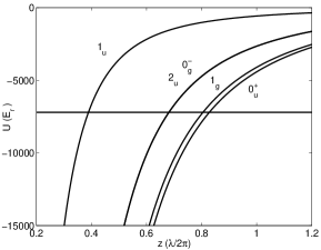
FIG. 5.: The shifted ground state and the attractive excited state [labeled by Hund’s case (c) notation] molecular potentials of Cs for $\delta=-3.0\Gamma$.

V Monte Carlo wave function method

In this section we describe briefly the main features of the Monte Carlo wave function (MCWF) method [14] which was developed for problems in quantum optics and discuss the implementation of the method to solve the cold collision problem in optical lattices.

A Basic Monte Carlo method

Various types of Monte Carlo (MC) methods [14, 15, 16] have been developed for problems where a direct analytical or numerical quantum mechanical solution of the density matrix Master Equation is very difficult or impossible due to the complexity of the problem. Complexity usually arises because of the coupling of the system studied to a reservoir with a large number of degrees of freedom and also because of a large number of elements in the system density matrix. Problems of this kind are common in laser cooling of neutral atoms. Various types of quantum approaches are possible in 2D systems [23] but in 3D a full quantum treatment of laser cooling of atoms has only been given in terms of the Monte Carlo method [24].

The core idea of MCWF method is the generation of a large number of single wave function histories including stochastic quantum jumps of the system studied. Solutions for the steady state density matrix and system properties can then be calculated as ensemble averages of single histories.

To generate single histories of the system wave function $|\psi\rangle$, one solves the time-dependent Schrödinger equation

$$i\hbar\frac{\partial|\psi\rangle}{\partial t}=H|\psi\rangle.$$ (42)

Here the non–Hermitian Hamiltonian $H$ is

$$H=H_{S}+H_{DEC}$$ (43)

where $H_{S}$ is the system Hamiltonian, Eq. (8) in our case, and the non-Hermitian part $H_{DEC}$ includes the decay part. $H_{DEC}$ is constructed from appropriate jump operators $C_{j}$ corresponding to a decay channel $j$ and to the detection scheme of the system. The general form of the non-Hermitian part reads

$$H_{DEC}=-\frac{i\hbar}{2}\sum_{j}C_{j}^{\dagger}C_{j}.$$ (44)

During a time evolution step $\delta t$ the norm of the wave function may shrink due to $H_{DEC}$ and the amount of shrinking gives the probability of a quantum jump to occur during the short interval $\delta t$. Based on a random number one then decides whether a quantum jump occurred or not. Before the next time step is taken, the wave function of the system is renormalized. In the case that a jump occurs, one performs a rearrangement of the wave function components according to the jump operator $C_{j}$, corresponding to decay channel $j$, before renormalization of $|\psi\rangle$.

B Time evolution

A natural termination for a simulation occurs if a steady state appears. One must note that the time to reach steady state varies even for the same system studied when the laser parameters are changed. Therefore one has to be careful to have long evolution times to make sure that the steady state is reached and ensemble averaging can be done in a reliable way.

We solve the time–dependent Schrödinger equation Eq. (42) by the split operator–Fourier transform method [25]. Formally solving Eq. (42) over $\delta t$ gives

$$|\psi(t_{0}+\delta t)\rangle=U|\psi(t_{0})\rangle$$ (45)

where the time evolution operator U reads

$$U=\exp\left(-\frac{iH\delta t}{\hbar}\right).$$ (46)

We split the time evolution operator $U$ including the Hamiltonian $H$ of Eq. (43) into three parts as $H=H_{V}+H_{K}+H_{D}$. When $H$ is in matrix form, $H_{V}$ has an off-diagonal part accounting for the atom–field coupling and the interaction between atoms, $H_{K}$ is the diagonal kinetic part and $H_{D}$ includes the non-kinetic diagonal part, i.e., decay and detuning.

For non-commuting operators $A$ and $B$ we can write to second order accuracy [25]

$$\exp\left(A+B\right)\simeq\exp\left(A/2\right)\exp\left(B\right)\exp(A/2).$$ (47)

As we take many consecutive time steps during the evolution, we finally approximate the wave function at time $t_{0}+n\delta t$ by

$$|\psi(z,t_{0}+n\delta t)\rangle\simeq\left[\prod_{k=0}^{n-1}U_{V}U_{D}^{1/2}U_{K}U_{D}^{1/2}\right]|\psi(z,t_{0})\rangle.$$ (48)

Here, $U_{D}\!=\!\exp(-iH_{D}\delta t/\hbar)$ and $U_{K}\!=\!{\cal F}^{-1}\exp(-i\delta t\frac{\hbar k^{2}}{2M})$ where ${\cal F}$ and ${\cal F}^{-1}$ denote the Fourier and inverse Fourier transforms. Finally, $U_{V}$ can be written as $U_{V}=S\exp(D)S^{-1}$ where $S$ contains eigenvectors and $D$ eigenvalues of $H_{V}$. $U_{V}$ corresponds now to a change of basis, multiplication by exponentials of eigenvalues and change of basis back to the product state basis. The above form for the temporal evolution of $|\psi\rangle$ is straightforward to implement and fast on a computer, e.g., 20% faster than the Crank–Nicholson method.

C Decay channels

A single atom has six different ways to spontaneously emit a photon so the total number of decay channels is 12 for two atoms (channels $1-6$ for atom 1, $7-12$ for atom 2). For each decay channel, $j$, the jump probability is given by

$$P_{j}=\delta t\langle\psi|C_{j}^{\dagger}C_{j}|\psi\rangle,$$ (49)

where the jump operators $C_{j}$ are constructed from single particle jump operators. In the single particle subspace for atom $\alpha$ and decay channel $j$ we have

$$\widetilde{C}_{j}^{\alpha}=CG_{j}\sqrt{\Gamma}~{}|g_{\alpha}m_{\alpha}\rangle_{\alpha}~{}_{\alpha}\langle e_{\alpha}m_{\alpha}|,$$ (50)

where $e_{\alpha}m_{\alpha}$ labels the excited level from which, and $g_{\alpha}m_{\alpha}$ the ground level to which jump occurs. Extension to the product state basis is simple [19]: For atom 1, $C_{j}=\widetilde{C}_{j}^{1}\otimes\openone_{2}$, and for atom 2, $C_{j}=\openone_{1}\otimes\widetilde{C}_{j}^{2}$.

For example, if we denote the jump of atom 1 from $|e_{-1/2}\rangle_{1}$ to $|g_{-1/2}\rangle_{1}$ as channel 2, the jump operator in the product state basis for this jump is

$$C_{2} = \sqrt{2/3}\sqrt{\Gamma}\left\{|g_{-1/2}\rangle_{1}~{}|g_{-1/2}\rangle_{2}~{}_{1}\langle e_{-1/2}|~{}_{2}\langle g_{-1/2}|\right.$$ (56)

$$+|g_{-1/2}\rangle_{1}~{}|g_{+1/2}\rangle_{2}~{}_{1}\langle e_{-1/2}|~{}_{2}\langle g_{+1/2}|$$

$$+|g_{-1/2}\rangle_{1}~{}|e_{-3/2}\rangle_{2}~{}_{1}\langle e_{-1/2}|~{}_{2}\langle e_{-3/2}|$$

$$+|g_{-1/2}\rangle_{1}~{}|e_{-1/2}\rangle_{2}~{}_{1}\langle e_{-1/2}|~{}_{2}\langle e_{-1/2}|$$

$$+|g_{-1/2}\rangle_{1}~{}|e_{+1/2}\rangle_{2}~{}_{1}\langle e_{-1/2}|~{}_{2}\langle e_{+1/2}|$$

$$\left.\!+|g_{-1/2}\rangle_{1}~{}|e_{+3/2}\rangle_{2}~{}_{1}\langle e_{-1/2}|~{}_{2}\langle e_{+3/2}|\right\}$$

and the corresponding jump probability for channel 2 is

$$P_{2}=\frac{2}{3}\delta t\Gamma\left\{\right. |\psi^{e_{-3/2}}_{g_{-1/2}}|^{2}+|\psi^{e_{-3/2}}_{g_{+1/2}}|^{2}+|\psi^{e_{-3/2}}_{e_{-3/2}}|^{2}$$ (57)

$$+ \left.|\psi^{e_{-3/2}}_{e_{-1/2}}|^{2}+|\psi^{e_{-3/2}}_{e_{+1/2}}|^{2}+|\psi^{e_{-3/2}}_{e_{+3/2}}|^{2})\right\}.$$ (58)

We neglect here the case where both atoms jump and two photons are detected simultaneously. The probability for a single atom jump during $\delta t$ is $\ll 1$ so the joint jump probability is negligible compared to the single atom jump probability. In principle it would be possible in simulations to take into account joint jumps but this unnecessarily complicates the jump procedure. After applying the jump operator $C_{j}$, the wave function is still in a superposition state, but it has collapsed onto product state basis vectors, leaving only one ground state level component of the jumped atom populated.

D Ensemble averaging

We calculate the results as an ensemble average of single history time averages in the steady state time domain [16]. This averaging method requires a smaller number of histories calculated to achieve reasonable error bars than a simple ensemble averaging at a single steady state time point. In our study, extra complications arise because the number of collision processes in the whole ensemble also comes into play. Atoms do not end up in the same lattice site, producing collisions, in all the calculated histories. Atomic hopping between lattice sites is a stochastic process and only in a fraction of the total number of histories, collision processes occur. We need a sufficiently large ensemble to produce enough collision events to have reliable results. This is why we have a much larger ensemble size, $96-128$ members, than e.g. used in 3D laser cooling Monte Carlo simulations using the same ensemble averaging method [24].

TABLE III.: Characteristic units. Distances are given in nm, momenta in $10^{-28}$ kgm/s, time in ns, and energy in $10^{-30}$ J.

Quantity	Characteristic unit	Cs	Rb	Na
distance	$\lambdabar=1/k_{r}$	136	124	94
momentum	$p_{r}=\hbar k_{r}$	7.77	8.49	11.25
time	$\Gamma^{-1}$	193	167	99
energy	$E_{r}=(\hbar^{2}k_{r}^{2})/2m$	1.37	2.55	16.57

In order to be able to use this averaging method, we need to be sure that time averages of single histories have been calculated in the steady state time domain. The simulation times used are displayed in Table IV. We have carefully checked from the time evolution of the kinetic energy that the simulation time was long enough to reach well into the steady state time domain.

VI Simulation scheme

In this section we present the charasteristic units used in our calculations and discuss the various criteria which set the numerical limits for the simulations. The approximations used and the numerical details related to the wave packet initial conditions and dynamics are also presented.

A Scaling and discretization of space

It is useful from a practical point of view to choose suitable units and scale the time-dependent Schrödinger equation (42) accordingly. Convenient physical units and their numerical values for the three appropriate alkali metal elements are listed in Table III. In the discussion below, we list all quantities and scale equations in units of the characteristic quantities displayed in Table III unless explicitly stated otherwise.

TABLE IV.: Simulation times: Total time for collision simulations $T$, ensemble averaging time $T_{ave}$, time step size $\delta t$ and maximum momentum $|p|_{max}$ given by $\delta t$ for the numerics to remain reliable.

Simulation	$\displaystyle{T(\Gamma^{-1})}$	$\displaystyle{T_{ave}(\Gamma^{-1}s_{0}^{-1})}$	$\displaystyle{\delta t(\Gamma^{-1})}$	$\displaystyle{|p|_{max}(p_{r})}$
Cs374	1600	78-125	0.2	110
Cs584	1600	97-194	0.2	110
Cs1621	760	178-256	0.1	155
Rb560	1600	140-280	0.2	89
Na339	470	99-198	0.05	90
Na530	470	155-311	0.05	90

As the phase factor $\exp(-iE\delta t/\epsilon)$ has to be well defined, cf. Eq. (46), we obtain a criterion for the maximum size of the time step $\delta t$ dictated by the maximum kinetic energy since we should fulfill the relation $\delta t\ll\epsilon/p^{2}$. Here $\epsilon$ is the energy of the linewidth of the transition in recoil units, as previously displayed in Table I. Collisions increase the atomic kinetic energies which makes the criterion for $\delta t$ numerically more strict for the two–atom case, compared to the one–atom Sisyphus cooling simulation (cf. Fig. 3). We give in Table IV the values of $\delta t$ for various simulations and the maximum momentum $|p|_{max}$ for the numerics to remain reliable. The total simulation times are $125-311$ in units of $1/(\Gamma s_{0})$. These depend on the properties of the alkali metal elements and the laser parameters.

For the numerical simulations, one has to discretize the position and momentum spaces, and the resolution has to be fine enough to ensure valid results. We have used 8192 grid points when the length of the entire spatial grid is $L_{z}=5\lambda\simeq 31.4\lambdabar$. This gives the step sizes in position and momentum spaces of $\delta z\simeq 0.0038$ and $\delta p=0.2$. The width of the Gaussian wave packet at the beginning of the simulation is $\Delta z_{0}=0.02\lambda\simeq 0.1257\lambdabar$ giving $\Delta z_{0}/\delta z\simeq 33$ and in momentum space $\Delta p_{0}/\delta p\simeq 20$, ensuring sufficiently fine resolution.

The inverse space (here momentum space) has reflecting boundary conditions when using the FFT method. Thus the size of the momentum space has to be large enough to avoid the reflection of high kinetic energy atoms at the edges of the momentum space. This requires special attention when considering the interaction simulations where the kinetic energies of the atoms increase due to the inelastic collisions.

The momentum space grid has a total size of $L_{k}=2\pi/\delta z=1638$ so that the atomic momenta may have values $|p|\leq 819$. The depths of the lattices in our simulations are such that atoms localized at a lattice site have momenta $|p|<50$. The momenta increase when the atoms wander around in the lattice, especially due to the inelastic collisions. The probability of gaining a sufficient momentum to reach the edge of our momentum space grid in a single collision event is now negligible. On the other hand many consecutive collisions do not shift the population for large $p$ and the reflection effect is avoided. This is due to the fact that the increasing relative velocity between the atoms reduce the excitation probability and increases in momentum terminate before the edges of the $p$–space are reached.

B Position fixing of one atom

We simulate the behaviour of a 36 level dissipative quantum system with a position-dependent coupling to the laser field and a position-dependent coupling between two atoms. This requires large computational resources. With the current computer capacity, it is not possible to simulate the situation where both atoms are allowed to move freely. Instead we have to fix one atom spatially and let only the other atom move. This reduces the dimensionality of the problem to one since the relative position of the atoms with respect to the laser field is now fixed. This also means that an inelastic interaction process will not change the kinetic energy for both atoms, but we use the relative kinetic energy as an estimate for the kinetic energy change per atom.

In our previous study [9] the position of the fixed atom was kept constant but here we relax this condition. The position $z_{f}$ of the fixed atom is now selected randomly in the interval $|z_{f}|<0.125\lambda$ for each ensemble member. This range covers all the interesting physics as an atom fixed outside the current range would be rapidly optically pumped to the opposite lattice well and the situation would correspond to that with the above-mentioned range of $z_{f}$.

The change of $z_{f}$ also moves the Condon point $r_{c}$ with respect to the lattice and now $r_{c}$ may be located anywhere between the lattice well and peak. This is an important point for making our model more realistic: Since the kinetic energy of the atom changes when it moves in the periodic optical potential, the relative velocity between the atoms and thus the excitation probability to the attractive molecular state at $r_{c}$ depends on its position in the lattice. When $r_{c}$ is located at the peak of the optical potential, the atom has to move up the potential hill to reach it. The relative velocity between the two atoms is now less and the excitation probability higher than in the case where the location of $r_{c}$ is at the bottom of the optical potential.

C Initial wave packet

At the beginning of the simulation, the wave packet is placed in a randomly chosen ground state sublevel. The initial Gaussian packet has a full spatial width of $0.02\lambda$. Thus the initial position of the spatially relatively narrow wave packet in the lattice is random but completely out of the range of the molecular resonance.

Each wave packet has a randomly selected mean initial velocity given by the Maxwell-Boltzmann distribution corresponding to the selected initial temperature of the atomic cloud. We emphasize that the momentum space width of the initial wave packet has no association with the thermal distribution, as it is merely needed to satisfy the Heisenberg uncertainty relation for a spatially localized initial state. As stated above, the connection between the wave packet and the temperature takes place via the mean momentum of the wave packet. By selecting this mean momentum randomly for each ensemble member but weighting the occurrences with the Maxwell-Boltzmann distribution, we create within the Monte Carlo ensemble another ensemble of possible initial collision velocities. This is the wave packet version of the standard collisional energy average [26].

As mentioned above only the ensemble averaged momentum probability distribution has a relation to temperature. This initial distribution gets narrower when the system evolves and the simulation progresses corresponding to cooling of the whole atomic cloud. Moreover, it must be stressed that the steady state reached does not depend on the initial widths of the single wave packets nor on the initial temperature as long as the atoms are in the reach of Sisyphus cooling. The simulation times get longer when the initial temperature is increased but we want to take into account the effect of collisions on the cooling dynamics in a realistic way. We also note that the steady state after cooling in the lattice does not necessarily correspond to a Maxwell–Boltzmann distribution of velocities but a clear steady state corresponding to the lattice properties is still reached [18].

It should be noted that although we include by default the recoil effects by absorption and stimulated emission, we cannot in our quantum approach take proper account of the Doppler shift which is the basis of the semiclassical description of Doppler cooling [27]. So in practice we neglect the Doppler cooling mechanism. Adding the recoil from spontaneous emission will not change this fact, nor the simulation results. In any case, the role of Doppler cooling is negligible when compared to the Sisyphus cooling force for the velocities of atoms localized in the lattice [4]. It can, however, have a role in the recapture of the hotter atoms heated by collisions, so in that sense our model is limited.

D Occupation density of lattice

We have performed all the simulations presented in this paper for an occupation density of $\rho_{o}=25\%$ in one dimension, whereas in our earlier work [9], we presented also results for other one-dimensional densities in Cs lattices. These previous simulations showed that an occupation density of 25% is sufficiently high for interesting effects to appear, namely an evaporative cooling process which works for at least some parameters of the laser field. The occupation density used in this paper is also nearly the largest density we can use when the simulations are done in the way presented here. The purpose of the paper is to further explore the parameter space and to extend our simulations to other atomic masses in addition to describing the details of our simulation approach.

For $\rho_{o}=25$% the available spatial length for the moving atom should be equal to $\lambda$, corresponding to the average distance between the atoms. But decreasing the spatial size increases the step size in the momentum space since $\delta p=2\pi/L_{z}$. So to have a sufficiently fine resolution in momentum space and still keep $\rho_{o}=25\%$, we choose $L_{z}=5\lambda$ and set an elastic repulsive potential barrier such that the allowed spatial length is $\lambda$. The forbidden spatial region thus makes the numerics work properly without altering the physics. Of course the forbidden region does not affect the momentum space.

Every fourth lattice is occupied when $\rho_{o}=25$% or in other words there is 1 atom per wavelength $\lambda$. This corresponds to a situation where the fixed atom sits e.g. at $z=0$ and the repulsive elastic potential barrier for the moving atom is set at $z=\lambda$. Then two consecutive collisions are described when the moving atom travels from the first collision region to the repulsive barrier, turns back, and collides again. Memory effects from previous collisions are rapidly removed due to decoherence, as also discussed in Sec. III. This is why we can say that the present model describes collisions in general in a lattice and not only between the same two atoms.

The dimensionality of the problem and the position fixing of one atom causes subtleties related to the occupation density: The moving atom travels on average a distance of $1\lambda$ for the first collision. After this event it has to travel a distance $2\lambda$ (from $z_{f}$ to $z_{f}+1$ and back) to collide again. The probability is high for a large kinetic energy increase during the first collision. Thus the first collision has the dominant effect on the kinetic energy scale relevant to the lattice dynamics. This is why we rather use here $\rho_{o}=25\%$ which corresponds to the average collision distance of $1\lambda$.

It is not trivial to connect the one-dimensional occupation density to the two- or three-dimensional density, as that will depend on the particular form of the lattice. It suffices to note, though, that a certain occupation density in one-dimension will typically correspond to a lower value in higher dimensions, so that e.g. in three dimensions we expect to see the effects studied here for three-dimensional occupation densities less than 25%.

E Interaction at short range

The DDI , Eq. (41), becomes singular at short range. The singularity in $H_{V}$ is simply removed by replacing $r$ with $r+r_{\rm off}$ and choosing $r_{\rm off}=10^{-8}$. When constructing the time evolution operator $U$, we diagonalize $H_{V}$ and the DDI part in $H_{V}$ produces the eigenvalue manifolds corresponding to the attractive and repulsive molecular potentials.

We replace the position dependencies of the attractive states which are the same as in $V_{dip}^{axis}$, Eq. (41), by

$$\frac{1}{r^{n}}\rightarrow\frac{1}{(r^{b}+r_{\rm off})^{n/b}},\,(n=1,2,3)$$ (59)

in a manner similar to what was done in Ref. [7]. Table V gives the used values of $b$, and we show the potentials in Fig. 6.

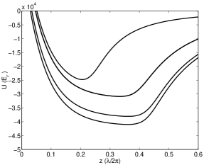
FIG. 6.: The short range attractive excited molecular potentials for Cs. Repulsion of exponential form has been added and the deep part of the potentials flattened to allow reliable numerical treatment of momentum (see text).

The main reason for this ”flattening” of the attractive state potentials is that considering the numerics, we have an upper limit to momentum. Thus we need to set a maximum momentum which can be reached in our simulations by acceleration, but which can still be treated reliably numerically in our integration grid, and is nevertheless large enough to correspond to a clear loss process. By selecting different values for $b$ for each molecular potential we take into account the individual characteristics of the different attractive states and of the atomic elements. It should be noted that by the time the atoms reach the artificially modified part of the attractive potentials, they move fast enough to make decay unlikely before they are reflected and move again to the region where the modification does not affect the potentials Thus the flattening of the potentials does not increase the time the atoms spend inside the modified part of the potential, i.e., this does not enhance radiative decay artificially.

We concentrate on the radiative heating which occurs because of the strong decay in the vicinity of $r_{c}$. In this region the treatment of the singularity in the DDI and in the attractive molecular states does not yet affect the potentials. For example, the removal of the singularity causes a change in the value of the Cs $0_{u}^{+}$ potential of 0.7% at the position $r=0.50$ when $r_{c}\simeq 0.83$ for the detuning used, $\delta=-3\Gamma$.

TABLE V.: Values of $b$. Numerical values which are used for the various attractive molecular states and atomic species. See also Eq. (59) and Figs. 5 and 6.

element	$0^{+}_{u}$	$1_{g}$	$0_{g}^{-}$	$2_{u}$	$1_{u}$
Cs and Rb	22	22	20	20	13
Na	13.5	13.5	12.5	12.5	10

The atoms repel each other at the very short range when their electron clouds begin to overlap. We do not have to consider the details of the short range repulsion. Thus the short range repulsion is simply produced by adding the exponential term $\alpha\,\exp(-\beta r)\,\epsilon$ to the eigenvalues of $H_{V}$. For flat states (states other than attractive or repulsive excited states) $\alpha=30$, $\beta=20$ for Cs and Rb, $\alpha=100$, $\beta=20$ for Na [28]. For the attractive excited state eigenvalue manifolds $\alpha=25$, $\beta=15$ for Cs and Rb, $\alpha=90$, $\beta=15$ for Na. Values of $\alpha$ and $\beta$ are chosen such that they produce high enough repulsion within a sufficiently short range but without producing numerical difficulties because of the contradictory requirements of height and range.

Finally we emphasize that apart from flattening the potentials, we perform our calculations in the atom-atom basis. Thus the molecular states are not used directly. Unfortunately our dipole-dipole potential takes care only of the force part of the atomic interaction. The $r$-dependence of the lifetimes of the molecular states are ignored, i.e., each molecular state ends up having the constant atomic linewidth, instead of the retarded linewidth. This linewidth arises from the fact that the two atoms couple to the same vacuum modes at different locations, leading to an $e^{-i\vec{k}\cdot\vec{r}}$ phase difference term. However, the atomic lifetimes differ at maximum only by a factor of 2 from the atomic one. The main exception is the 2_u state, which becomes strongly dipole-forbidden and can support strong survival and thus e.g. favor the fine structure change loss mechanism over the radiative process. But we have typically $r_{c}\lesssim 0.8\lambdabar$, which means that the 2_u state is already hard to excite as well (see Ref. [26] for a detailed discussion). In order to make the quantum jump process tractable we use the atom-atom basis, and, unfortunately, we can not just transform into the molecular basis, change the linewidths into retarded ones, and then transfer into the atom-atom basis (as we do when flattening the potentials). This is because for decay, the lifetimes appear in the jump operators in addition to the Hamiltonian.

F Atoms escaping the lattice

One needs to define the critical momentum $p_{c}$ to be able to calculate the MC ensemble averages and the properties of the atoms remaining in the lattice. If $|p|<p_{c}$ atoms are considered to remain/relocalize in the lattice, whereas when $|p|\geq p_{c}$ they are considered lost from the lattice due to a collision or a series of collisions. Semiclassically, we can calculate the critical $p^{sc}_{c}$ where the cooling force has its maximum value for the parameters used [4]. The cooling force is, of course, still effective for momenta above $p^{sc}_{c}$.

Due to the stochastic nature of the jumps, it is not possible to say if a given high momentum atom will relocalize or if it is lost from the lattice. Assume that an atom has a momentum $|p|>p^{sc}_{c}$. If the following few quantum jumps reduce the kinetic energy of the atom, depending on the atomic position in the lattice, it has a good chance to relocalize in the lattice. In the opposite case, where the next few jumps increase the kinetic energy of the atom, corresponding to jumps from the vicinity of the bottom of the potential well to the vicinity of the top of the well, the atom has less probability to relocalize into the lattice. This means that for two different MC histories with the same initial value of $|p|>p^{sc}_{c}$ one atom may escape from the lattice whereas the other one may relocalize. Thus it is not possible to define $p_{c}$ in a way that all atoms below $p_{c}$ always relocalize while when $|p|\geq p_{c}$ they escape.

When we calculate the kinetic energy per atom staying in the lattice, we need a criterion for neglecting those MC histories in the ensemble averaging that correspond to atoms lost from the lattice. To solve the problem, we have calculated the kinetic energy per atom by using various values of $p_{c}$. Since there is an increase in the average kinetic energy as a function of time when the value of $p_{c}$ used is too large, we may check from the time evolution of the kinetic energy that our choice for $p_{c}$ is the proper one when we want to calculate the average kinetic energy per atom in the lattice. This is because more collisions occur as the system evolves in time and if the gain in kinetic energy is too large for the atoms to relocalize in the lattice, the kinetic energy increases as a function of time and no steady state is reached, as demonstrated in Fig. 7. Whereas when we use an appropriate value for $p_{c}$, atoms still relocalize in the lattice and the kinetic energy exhibits a steady state behaviour, cf. Fig. 8. It is at the transition point between these two different types of behaviours of the kinetic energy that we should choose the correct value for $p_{c}$.

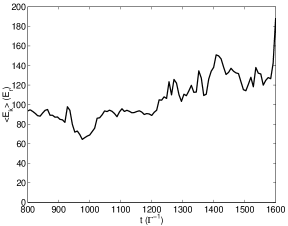
FIG. 7.: Kinetic energy time evolution indicating a too large choice for $p_{c}$. The steady state is not reached since collisions increase the kinetic energy and the collided atoms are out of the recapture range, and thus escape from the lattice. (Cs584, $p_{c}=60$).

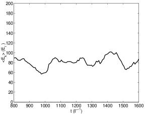
FIG. 8.: Kinetic energy time evolution indicating a steady state. Atoms above the recapture range are now omitted with the proper choice for $p_{c}$. (Cs584, $p_{c}=40$).

Consequently, the atoms of a kinetic energy exceeding the limit given by $p_{c}$ are neglected when we perform the ensemble averaging to find the result for the kinetic energy per atom remaining in the lattice. It is important to note that the main result related to the narrowing of the momentum probability distribution due to collisions still includes all the calculated histories and is totally independent of $p_{c}$.

If there is no constant injection of atoms into the lattice, collisions slowly deplete it. Finally the density is sufficiently low that the interactions between atoms are negligible and the atomic cloud regains the properties determined by the laser parameters only. It should thus be realized that what we describe here is a temporary cooling process which is not effective when the density has decreased. What we emphasize is the unexpected behaviour of the system in the intermediate regime where the effect of collisions is not heating but cooling. This does not represent the nature of the complete dynamics of the atomic cloud, of course, as there are other mechanisms, such as the radiation pressure from scattered photons, for both heating and cooling, which are not included here.

G Computational resources

The numerical simulations are demanding since we are dealing with a 36 level quantum system including various position dependent couplings and dissipative coupling to the environment. We use 32 processors of an SGI Origin 2000 machine which has 128 MIPS R12000 processors of 1 GB memory per processor [29]. The total memory taken by a single simulation (fixed $\delta$, $\Omega$, $\rho_{o}$ and atomic species) is 14 GB and generating a single history requires 6 hours of CPU time. A simulation of 128 ensemble members then requires a total CPU time which is roughly equal to one month. The normal clock time is, of course, much shorter (roughly 22 hours) since we take advantage of powerful parallel processing.

VII The Semiclassical Approach

In this section we describe the semiclassical approach to calculate the excitation and survival probabilities on the molecular excited states of our two-atom system.

A Landau–Zener formula and classical path approximation

One can calculate the semiclassical excitation probability of the wave packet traveling through the crossing region between the two states of the system by using the Landau–Zener formula

$$P_{LZ}=1-\exp(-\pi\Lambda)$$ (60)

where $\Lambda$ includes both the coupling between the two states and the $C_{3}$ factor which gives the inverse cubic $r$-dependence of the excited state ($C_{3}/r^{3}$) [2]. The basic idea here is that the short resonance region is approximated to consist of two spatially linearly behaving states and each component of the wave packet arriving at the resonance region is independently excited. A more detailed description can be found in Ref. [2].

One can then calculate the time it takes to reach a point $r$ on the excited state by using the classical path approximation

$$t=t(r)=-\int_{r_{c}}^{r}dr^{\prime}\left[\frac{2}{m}\left(\frac{p_{cr}^{2}}{2m}+\frac{C_{3}}{r^{\prime 3}}-\hbar\delta\right)\right]^{-1/2}$$ (61)

where $p_{cr}$ is the momentum at the Condon point $r_{c}$. There is a direct correspondence between the reached point $r$ on the excited state and the energy gain while accelerating on the attractive excited molecular state. By using Eq. (61) one can calculate classically how long it takes to reach a point $r$ corresponding to a given increase in kinetic energy or momentum due to the acceleration on the attractive excited state.

It is now easy to numerically calculate the kinetic energy increase due to the collisions if the wave packet stays on the attractive excited state for a time corresponding to the natural decay time $\Gamma^{-1}$. When the exponential decay from the excited state is also taken into account, the probabilities for various kinetic energy gains due to collisions as a function of relative velocity of the colliding atoms at $r_{c}$ may also be calculated [7].

TABLE VI.: Semiclassical probabilities to gain kinetic energies on various attractive excited state molecular levels, see Fig. 5, for our $Cs584$ simulation. The probabilities are calculated for $p_{tot}=p_{cr}+\Delta p=40$ and $p_{cr}=24$, this value of $p_{cr}$ corresponds to the lattice depth. The wave packet spends a time $t\geq t_{e}$ on the excited state, $P_{LZ}$ is the Landau-Zener excitation probability and $P_{a}$ gives the survival probability. $P_{tot}=P_{a}P_{LZ}$ is the total semiclassical probability for the process $p>p_{tot}=40$ to occur.

potential	$\displaystyle{t_{e}(\Gamma^{-1})}$	$\displaystyle{P_{LZ}}$	$\displaystyle{P_{a}}$	$\displaystyle{P_{tot}}$
$1_{u}$	0.21	0.71	0.81	0.57
$2_{u}$,$0^{-}_{g}$	0.40	0.88	0.67	0.59
$1_{g}$	0.48	0.91	0.62	0.57
$0^{+}_{u}$	0.49	0.92	0.61	0.56

B Post collision momentum in the lattice

We obtain the values of $C_{3}$ for the attractive potentials by fitting near the resonance region the simple expression $-C_{3}/r^{3}$ to our molecular potentials obtained by diagonalizing the dipole–dipole coupling presented in the two–atom basis, Eq. (41). Figure 9 shows an example of the total post collision momentum $p_{tot}=p_{cr}+\Delta p$ as a function of $p_{cr}$ when the wave packet spent a time $t=\Gamma^{-1}$ on the $1_{u}$ excited state ($Cs584$). One notices that $p_{cr}=24$ corresponding to the lattice depth used already gives a total momentum of $p_{tot}=67$ after a collision thus pushing the atom to the region in momentum space where its probability for relocalizing back to the lattice is small ($p_{c}^{sc}=16.2$). This shows in a clear way that increases in kinetic energy that are large compared to the latttice modulation depth $U_{0}$ may occur on a time scale of $\Gamma^{-1}$.

FIG. 9.: The total momentum $p_{tot}=p_{cr}+\Delta p$ as a function of resonance point momentum $p_{cr}$ for the attractive $1_{u}$ state by the semiclassical calculation. The wave packet has spent a duration corresponding to $\Gamma^{-1}$ accelerating on the excited state before spontaneous decay back to the ground state. (Cs584).

Moreover, when the exponential decay and $P_{LZ}$, Eq. (60), are taken into account, one is able to calculate the probabilities to gain various amounts of kinetic energies due to the collision. The total probability $P_{tot}$ for the atomic momentum to have at least the value $p_{tot}$ after the collision is

$$P_{tot}=P_{a}P_{LZ}$$ (62)

where $P_{a}$ gives the survival probability on the excited state. An example of the results of $P_{tot}$ are shown in Table VI. This suggests that the first resonance molecular potential $0^{+}_{u}$ has a dominant role in collisions. For $p_{tot}=40$ the probabilities for the various states are roughly equal but if the first resonance potential excites and accelerates half of the colliding atoms only half of them is left for the remaining potentials.

The simple semi-classical calculation above is not able to give quantitative results but it shows that the probability to produce an atom of large momentum due to a collision is high already when we consider one excited level only. This probability increases when we take into account that during one collision process, the molecule may be excited at four different values of $r_{c}$ related to five different attractive states.

VIII Simulation Results

The calculated numerical values of kinetic energy per atom for various simulations are shown in Table VII and corresponding momentum probability distributions in Figs. 10–15.

Most of the simulations with the selected parameters produce a reduced value for the kinetic energy per atom when the interactions between the atoms are taken into account, see Table VII. Since the inelastic collisions here always increase the kinetic energy of the atoms via the radiative heating mechanism, our results suggest that the consequence of collision almost every time is the escape of the colliding high energy atoms from the lattice [30]. The atoms left in the lattice then have less average energy. This is due to the fact that the more energetic atoms are favoured to participate in the collision process due to their better ability to move between the lattice sites.

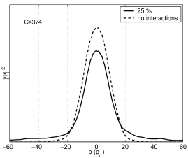
FIG. 10.: Momentum probability distributions for interacting and non–interacting cases. (Cs374).

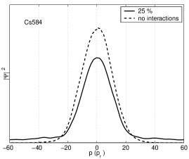
FIG. 11.: Momentum probability distributions for interacting and non–interacting cases. (Cs584).

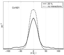
FIG. 12.: Momentum probability distributions for interacting and non–interacting cases. (Cs1621).

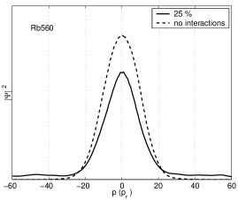
FIG. 13.: Momentum probability distributions for interacting and non–interacting cases. (Rb560).

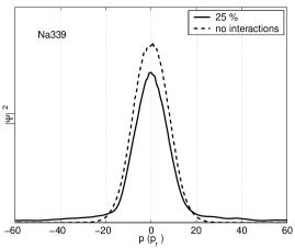
FIG. 14.: Momentum probability distributions for interacting and non–interacting cases. (Na339).

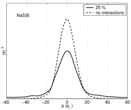
FIG. 15.: Momentum probability distributions for interacting and non–interacting cases. (Na530).

The cooling process is indeed observed when looking for the momentum probability distributions including all the MC histories for ensemble averaging, see Figs. 10–15. One can see the slight narrowing of the momentum distributions corresponding to the cooling process. The narrow central peak corresponds to atoms localized in the lattice sites and the broader background wing to atoms which are above the recapture range and do not relocalize in the lattice. This resembles the evaporative cooling process with narrowed central peak and hot background atoms. Cooling here is not dramatic but still present. Moreover, the result is in sharp contrast when compared to the theoretical and experimental collision studies in MOT’s where the heating of the trapped atoms due to the radiative mechanism is observed [2, 7] but not the evaporative-type cooling process.

The cooling process is observed for all the three atomic masses when similar lattice depths are used. The computational resources that simulations require, see Sec. VI G, do not allow any extensive exploration of parameter space but the Cs1621 result shows that with a deeper lattice the situation may change, see Table VII. In shallow lattices the relative velocity before a collision is small, thus enhancing the excitation probability. In deep lattices the reduced excitation probability due to large relative velocity is compensated by the use of more intense lasers. The Cs1621 result suggests that in deeper lattices one may observe heating which is similar to the results from MOT studies. But a systematic study of this is out of the reach of this paper.

TABLE VII.: Expectation values of kinetic energy per atom ($<E_{k}>$) for the simulations. The value of $p_{c}$ gives the critical momentum which is used in ensemble averaging to neglect atoms which have escaped from the lattice. The absolute values of the standard deviation are given in parentheses.

Simulation	$\displaystyle{p_{c}}$	$\displaystyle{<E_{k}>(E_{r})}$	$\displaystyle{<E_{k}>(E_{r})}$
		interactions	no interactions
Cs374	35	62 (5)	75 (5)
Cs584	55	82 (6)	110 (7)
Cs1621	70	264 (30)	221 (18)
Rb560	50	86 (8)	95 (5)
Na339	40	46 (3)	59 (3)
Na530	45	63 (6)	84 (6)

IX Discussion and Conclusions

Our results show the basic aspects of one mechanism affecting the thermodynamics of the atomic cloud in an optical lattice, when the lattice has been prepared with near-resonant (detuning a few linewidths), red-detuned laser light. In this case the role of inelastic collisions is strong, leading to heating and loss of atoms, but this requires that the interacting atoms are located in the same lattice site. This, on the other hand, requires, firstly, large atomic densities. Therefore in most lattice studies done so far, the role of collisions has been negligible due to the low densities, or at least not easy to observe (with the exception of collisions producing a clear signal such as Penning ionisation of colliding metastable rare gas atoms [31]).

Secondly, frequent collisions require clear mobility of atoms. This takes place naturally during the Sisyphus cooling until the atoms are localized in lattice sites. Thus it is important for suitably dense samples to study the role of collisions during the Sisyphus cooling, and our approach provides a method which is both dynamical and consistent. For the selected parameters our simulations show that the Sisyphus cooling process and localization of atoms is not prohibited by inelastic processes, i.e., the loss and heating of atoms remains small even when the average distance between the two atoms is only four lattice sites.

Once the localization in lattice sites has been achieved as a steady state, the question about the mobility of atoms changes to some extent. It should be noted that localization does not mean that an atom remains in the same site ad infinitum. In the steady state the atoms are localized at the sites for most of the time, but also move between the sites via tunneling (in the picture where the lattice lasers and the excited states are eliminated from the effective description). For the selected parameters the dipole-dipole interaction does not perturb the lattice potentials enough to have a significant effect between atoms located at different sites (the opposite situation is also possible, see Ref. [11]). The tunneling of atoms between sites is in the steady state the main process leading to inelastic collisions, and as the simulations show (supported by the semiclassical estimates) such encounters lead mainly to loss of hotter atoms or their selective heating. This is because the hotter atoms, naturally, move between the sites more frequently than the colder ones, creating the selectivity. If the lost atoms are not considered, our results show, however, that we can hold on to the concept of an existing steady state.

The collisionally induced velocity-selective loss of hot atoms is similar to the evaporative cooling which is utilised in magnetic traps to reach ultracold temperatures for atoms. It remains to be seen, however, whether the resulting cooling effect for the atoms is significant enough to be observed in densely filled lattices. In dense samples other processes such as reabsorption of photons scattered by the atoms are another important source for heating, which may well overcome any cooling effect. It should be noted, however, that if we ignore the spatial structure of the cooling fields, the collisional processes lose their velocity-selective nature, and as seen in the simulations of Ref. [7], this leads to strong heating of atoms. Here the simulations indicate that the lattice structure inhibits this heating clearly.

Our simulations have been very intense computationally, which makes it very difficult to make the model more realistic. Our studies, however, to our opinion, demonstrate the basic features to be expected from the collisions in densely populated near-resonant red-detuned lattices. There are magnetic-field-assisted cooling schemes for blue-detuned lattices for e.g. $J=1\rightarrow J=1$ systems. The blue detuning usually leads to optical shielding, and the collisional contribution to inelastic processes is reduced strongly for normal laser cooling intensities as the loss channel is expected to be adiabatically closed, see Ref. [32]. As a future prospect it will be interesting to study the qualitative differences due to the color of the detuning in collisions between atoms in near-resonant lattices.

- [1] H. J. Metcalf and P. van der Straten, Laser Cooling and Trapping, (Springer, Berlin, 1999).
- [2] K.-A. Suominen, J. Phys. B 29, 5981 (1996); J. Weiner, V. S. Bagnato, S. Zilio, and P. S. Julienne, Rev. Mod. Phys. 71, 1 (1999).
- [3] Y. Castin and J. Dalibard, Europhys. Lett. 14, 761 (1991).
- [4] J. Dalibard and C. Cohen-Tannoudji, J. Opt. Soc. Am. B 6, 2023 (1989); P. J. Ungar, D. S. Weiss, E. Riis, and S. Chu, J. Opt. Soc. Am. B 6, 2058 (1989).
- [5] P. S. Jessen and I. H. Deutsch, Adv. At. Mol. Opt. Phys. 37, 95 (1996); D. R. Meacher, Contemp. Phys. 39, 329 (1998); S. Rolston, Phys. World 11 (10), 27 (1998); L. Guidoni and P. Verkerk, J. Opt. B 1, R23 (1999).
- [6] D. Jaksch, C. Bruder, J. I. Cirac, C. W. Gardiner, and P. Zoller, Phys. Rev. Lett. 81, 3108 (1998); D.-I. Choi and Q. Niu, Phys. Rev. Lett. 82, 2022 (1999); M. T. DePue, C. McCormick, S. L. Winoto, S. Oliver, and D. S. Weis, Phys. Rev. Lett. 82, 2262 (1999); A. J. Kerman, V. Vuletić, C. Chin, and S. Chu, Phys. Rev. Lett. 84, 439 (2000).
- [7] M. J. Holland, K.-A. Suominen, and K. Burnett, Phys. Rev. Lett. 72, 2367 (1994); Phys. Rev. A 50, 1513 (1994).
- [8] P. S. Julienne and J. Vigué, Phys. Rev. A 44, 4464 (1991).
- [9] J. Piilo, K.-A. Suominen, and K. Berg-Sørensen, J. Phys. B 34, L231 (2001).
- [10] E. V. Goldstein, P. Pax, and P. Meystre, Phys. Rev. A 53, 2604 (1996).
- [11] C. Boisseau and J. Vigué, Opt. Commun. 127, 251 (1996).
- [12] A. M. Guzmán and P. Meystre, Phys. Rev. A 57, 1139 (1998).
- [13] C. Menotti and H. Ritsch, Phys. Rev. A 60, R2653 (1999); Appl. Phys. B 69, 311 (1999).
- [14] J. Dalibard, Y. Castin, and K. Mølmer, Phys. Rev. Lett. 68, 580 (1992); K. Mølmer, Y. Castin, and J. Dalibard, J. Opt. Soc. Am. B 10, 524 (1993).
- [15] M. B. Plenio and P. L. Knight, Rev. Mod. Phys. 70, 101 (1998) and references therein.
- [16] K. Mølmer and Y. Castin, Quantum Semiclass. Opt. 8, 49 (1996).
- [17] K.-A. Suominen, Y. B. Band, I. Tuvi, K. Burnett, and P. S. Julienne, Phys. Rev. A 57, 3724 (1998).
- [18] Y. Castin, J. Dalibard, and C. Cohen-Tannoudji, in Proceedings of Light Induced Kinetic Effects on Atoms, Ion and Molecules, edited by L. Moi et al., (ETS Editrice, Pisa, 1991).
- [19] C. Cohen–Tannoudji, B. Diu, and F. Laloë, Quantum Mechanics Vol. I (Wiley–Interscience, Paris, 1977), Chapter II F.
- [20] K. I. Petsas, G. Grynberg, and J.-Y. Courtois, Eur. Phys. J. D 6, 29 (1999) and references therein.
- [21] G. Lenz and P. Meystre, Phys. Rev. A 48, 3365 (1993).
- [22] P. R. Berman, Phys. Rev. A 55, 4466 (1997).
- [23] K. Berg-Sørensen, Y. Castin, K. Mølmer, and J. Dalibard, Europhys. Lett. 22, 663 (1993); Y. Castin, K. Berg-Sørensen, J. Dalibard, and K. Mølmer, Phys. Rev. A 50, 5092 (1994).
- [24] Y. Castin and K. Mølmer, Phys. Rev. Lett. 74, 3772 (1995).
- [25] B. Garraway and K.-A. Suominen, Rep. Prog. Phys. 58, 365 (1995) and references therein.
- [26] M. Machholm, P. S. Julienne, and K.-A. Suominen, Los Alamos archive, physics/0103059, to appear in Phys. Rev. A (2001).
- [27] S. Stenholm, Rev. Mod. Phys. 58, 699 (1986).
- [28] These are also the values used for all the states (for Cs, Rb and Na respectively) to produce the needed reflective boundary conditions by the repulsive exponential potential barrier. When using the Crank-Nicholson method to solve Eq. (42) it is easy to use the reflecting boundary conditions. Instead we use the FFT-method since it is computationally faster in the system studied here.
- [29] See http://www.csc.fi for details.
- [30] We have also estimated the number of collision processes by monitoring the quantum flux over average distance in single particle MC simulations. This estimate gives similar results as the number of high energy atoms produced when interactions between atoms have been included.
- [31] J. Lawall, C. Orzel, and S. L. Rolston, Phys. Rev. Lett. 80, 480 (1998).
- [32] K.-A. Suominen, M. J. Holland, K. Burnett, and P. S. Julienne, Phys. Rev. A 51, 1446 (1995).