Subthermal linewidths in photoassociation spectra of cold alkaline earth atoms

Abstract

Narrow $s$-wave features with subthermal widths are predicted for the ${}^{1}\Pi_{g}$ photoassociation spectra of cold alkaline earth atoms. The phenomenon is explained by numerical and analytical calculations. These show that only a small subthermal range of collision energies near threshold contributes to the $s$-wave features that are excited when the atoms are very far apart. The resonances survive thermal averaging, and may be detectable for Ca cooled near the Doppler cooling temperature of the 4¹P$\leftarrow$4¹S laser cooling transition.

I Introduction

Photoassociation spectroscopy has become a very powerful tool for studying the collision physics of laser cooled and trapped atoms [1]. The conventional wisdom is that the linewidth of individual molecular levels in the photoassociation spectra of laser cooled atoms is due to the natural linewidth plus thermal broadening on the order $k_{B}T$, where $k_{B}$ is the Boltzmann constant and $T$ is the temperature. Thus, we would not expect photoassociation lines to be much smaller than $k_{B}T$ in width [2, 3, 4, 5, 6, 7]. However, we demonstrate subthermal linewidths for a special case of photoassociation at very long range to an excited vibrational level $v$ with a small natural decay width $\Gamma_{v}$. In this case the $s$-wave vibrational features are very narrow at low $T$ (e.g., $<10$ $\mu$K), where $k_{B}T\ll\Gamma_{v}$. Surprisingly, such features can remain narrow even at much higher $T$ (e.g., $\approx$ 1 mK), where $k_{B}T\gg\Gamma_{v}$. These subthermal linewidths are a consequence of having only a narrow range of low collision energies that contribute to the thermally averaged photoassociation spectrum.

Narrow features are possible in ${}^{1}\Pi_{g}$ photoassociation trap loss spectra at small detuning of alkaline earth atoms in a magneto-optic trap (MOT) [8]. For Ca there is a good chance that the sharp $s$-wave features will stand out on a background comprised of broader peaks from the higher partial waves of the ${}^{1}\Pi_{g}$ spectrum and the broad features of the ${}^{1}\Sigma_{u}$ spectrum, even around the Doppler cooling temperature $T_{D}$ ($T_{D}=0.83$ mK for the Ca 4¹P$\leftarrow$4¹S cooling transition). Photoassociation spectroscopy in a Ca MOT has been reported [9], but in that experiment the photoassociating laser was detuned far from atomic resonance (about 780 atomic linewidths $\Gamma_{\rm at}$), whereas our features are predicted for small detunings ($<$ 25 $\Gamma_{\rm at}$).

II Theory of subthermal line shapes

A Trap loss spectrum

In Ref. [8] we outlined the numerical and analytical models used here. The numerical photoassociation trap loss spectrum is obtained from a fully quantum mechanical three-channel model, where the time-independent Schrödinger equation is solved with a complex potential to represent spontaneous decay from the excited state. We repeat only the essential analytical formulas here, and concentrate on the explanation of the phenomenon. For a more detailed description of different aspects of cold photoassociation collisions of alkaline earth atoms, see Ref. [8].

Figure 1 shows a high resolution scan of our calculated state change (SC) trap loss spectra of cold Ca atoms at three different temperatures for a single vibrational level of the ${}^{1}\Pi_{g}$ state. There are a number of ${}^{1}\Pi_{g}$ isolated vibrational resonance features in the range of detuning $\Delta$ from 1 to 25 $\Gamma_{\rm at}$ to the red of atomic resonance. Our example is typical of these features. Note that the features labeled $A$ and $B$ in the figure are both narrower than $k_{B}T_{D}$. Although the transition between the ${}^{1}\Sigma_{g}$ ground state and the ${}^{1}\Pi_{g}$ excited state is forbidden at short and intermediate internuclear distances $R$, it becomes allowed at long range due to relativistic retardation effects [8, 10]. The trap loss collision of the two cold atoms proceeds via excitation at a long range Condon point $R_{C}$ to the ${}^{1}\Pi_{g}$ state (the difference of ground and excited molecular potential energy curves equals the photon energy at $R_{C}$). Once in the ${}^{1}\Pi_{g}$ state the atoms are accelerated towards short range. The survival probability in moving from long to short range on the ${}^{1}\Pi_{g}$ state is close to unity due to the small decay rate ($\Gamma(R)\rightarrow 0$ for $R\rightarrow 0$). At short range a SC may occur due to spin-orbit coupling to a lower lying state correlating to atomic ¹S + ¹D, ³D or ³P states. After SC to these channels, modeled here by a single effective channel, the atoms will be lost from the trap due to the large gain in kinetic energy.

The photoassociation spectrum in Fig. 1 is the thermally averaged loss rate coefficient [11]:

$$K(T,\Delta) = \sum_{\ell_{even},J}(2\ell+1)\frac{\hbar\pi}{\mu}\left\langle\frac{|S_{pg}(\varepsilon,\Delta,\ell J)|^{2}}{k}\right\rangle$$ (1)

$$= \sum_{\ell_{even},J}\langle K(\varepsilon,\Delta,\ell J)\rangle.$$ (2)

Here $\varepsilon=\hbar^{2}k^{2}/(2\mu)$ is the collision energy at momentum $\hbar k$ for reduced mass $\mu$, $\ell$ is the ground state partial wave quantum number (0, 2, 4, …for identical Group II spinless bosons), $J=\ell,\ell\pm 1$ is the excited state rotational quantum number, and $\Delta$ is the detuning from the atomic resonance of the photoassociating laser. $S_{pg}(\varepsilon,\Delta,\ell J)$ is the $S$-matrix element for the transition between the ground state $g$ and the SC channel $p$ via the excited state $e$. The brackets $\langle\cdot\cdot\cdot\rangle$ imply a thermal average over a Maxwellian energy distribution:

$$\langle\cdot\cdot\cdot\rangle=\frac{2}{\sqrt{\pi}}\int_{0}^{\infty}x^{1/2}e^{-x}(\cdot\cdot\cdot)dx$$ (3)

where $x=\varepsilon/(k_{B}T)$. As we show below, a consequence of the excitation at a very large $R_{C}$ is that only a small range of energies, much less than $k_{B}T$ when $T$ is near $T_{D}$, contributes to the thermal average integral in Eq. (3), especially for $s$-waves. Consequently, averaging does not introduce much additional broadening.

FIG. 1.: Single vibrational feature of the Ca ${}^{1}\Pi_{g}$ photoassociation spectrum resulting in SC trap loss. The $\Delta/\Gamma_{\rm at}$ value where the peak appears depends on the model potentials in Ref. [8]. It may appear at a different $\Delta/\Gamma_{\rm at}$ in an actual experiment. The smooth background of about 2 units due to the ${}^{1}\Sigma_{g}\to{{}^{1}}\Sigma_{u}$ transition [8] is not shown. The Doppler cooling temperature for cooling on the 4¹P atomic state is 830 $\mu$K, and the recoil temperature is 2.7 $\mu$K. The low temperature limit for the feature labeled $A$ is a Lorentzian line centered at the resonance position $\Delta/\Gamma_{\rm at}=11.37$ with a natural width of 1.2 MHz. The peak of the $A$ feature, which clearly has a subthermal width for $T=830$ $\mu$K, is normalized to unity for the three different temperatures. The calculated peak trap loss rate coefficients for a 1 mW/cm² laser are $2\times 10^{-13}$ cm³/s (830 $\mu$K), $2\times 10^{-12}$ cm³/s (83 $\mu$K), and $8\times 10^{-12}$ cm³/s (8.3 $\mu$K), respectively.

B Analytic theory

An analytic interpretation can be given for the origin of the subthermal linewidths. When the spacing $h\nu_{v}$ between vibrational levels $v$ is much larger than their total width $\Gamma_{v}$, i.e., the vibrational resonances are non-overlapping, then $|S_{pg}|^{2}$ is given by an isolated Breit-Wigner resonance scattering formula for photoassociation lines [2, 4, 8]:

$$|S_{pg}(\varepsilon,\Delta,\ell J)|^{2} = {\Gamma_{vp}\Gamma_{vg}(\varepsilon,\ell J)\over\left[\varepsilon-{\cal E}_{v}(\Delta,J)\right]^{2}+\left({\Gamma_{v}/2}\right)^{2}}.$$ (4)

The total width $\Gamma_{v}$ is the sum of the decay widths into the SC ($\Gamma_{vp}$) and the ground state ($\Gamma_{vg}$) channels and the radiative decay rate ($\Gamma_{v,rad}$), and ${\cal E}_{v}(\Delta,J)=\Delta-[\varepsilon_{v}(J)+s_{v}(J)]$ is the detuning-dependent position of the vibrational level $vJ$ in the molecule-field picture relative to the ground state separated atom energy. The level shift $s_{v}(J)$ due to the laser-induced coupling [4] is small for our case. When $\Delta=\varepsilon_{v}(J)+s_{v}(J)$, then ${\cal E}_{v}(\Delta,J)=0$ and the vibrational level is in exact resonance with colliding atoms with zero kinetic energy.

In the reflection approximation $\Gamma_{vg}(\varepsilon,\ell J)$ is proportional to the square of the ground state wavefunction $\phi_{g}$ at the Condon point ($R_{C}$) [4, 12, 13]:

$$\Gamma_{vg}(\varepsilon,\ell J)=\frac{2\pi h\nu_{v}|V_{eg}(R_{C},\ell J)|^{2}}{D_{C}}|\phi_{g}(\varepsilon,\ell,R_{C})|^{2}.$$ (5)

Here $V_{eg}(R_{C},\ell J))$ is the laser-induced coupling, $D_{C}$ is the slope difference of the ground and excited state potentials at $R_{C}$, and $\nu_{v}$ is the vibrational frequency for level $v$. $|V_{eg}|^{2}$ is linear in laser intensity $I$ for our assumed weak-field case. Approximating the ground state wavefunction by its low-energy asymptotic form gives for $s$-waves

$$|\phi_{g}(\varepsilon,0,R_{C})|^{2}=\frac{2\mu}{\pi\hbar^{2}}\frac{\sin^{2}k(R_{C}-A_{0})}{k},$$ (6)

where $A_{0}$ is the scattering length of the ground state potential. For higher partial waves ($\ell>0$) [14],

$$|\phi_{g}(\varepsilon,\ell,R_{C})|^{2}=\frac{2\mu}{\pi\hbar^{2}}\frac{z_{C}^{2}|j_{l}(z_{C})|^{2}}{k},$$ (7)

where $j_{l}(z_{C})$ is the spherical Bessel function, and $z_{C}=kR_{C}$. The normal scattering phase shift does not appear in Eq. (7) since it is vanishingly small near threshold for the higher partial waves [1]. We define here the near threshold range of collision energies to be the range for which Eqs. (6) and (7) are good approximations.

FIG. 2.: Thermally averaged Ca SC trap loss rate for $T=$ 0.83 mK and $I=$ 1 mW/cm² from the analytic line shape model, Eqs. (4), (6) and (7), compared to the full quantum numerical result, including contributions from $\ell\leq 6$. The separate contributions are shown for the $s$-, $d$-, and $g$-waves, with the dominant contribution to each peak labeled by $\ell J$.

Figure 2 shows the thermally averaged Ca trap loss spectrum $K(T,\Delta)$ at $T_{D}=0.83$ mK obtained by inserting Eq. (4) into Eq. (1) using Eq. (6) or (7). The analytic model takes a few input parameters from the numerical model [8]: the scattering length for the ground state potential (the actual value is unknown, but the model value is 67 a₀), $\Gamma_{vp}/h\approx 0.3$ MHz $<\Gamma_{v,rad}/h=0.8$ MHz, and the position $\varepsilon_{v}(J)+s_{v}(J)$ of the vibrational levels for each $J$. The good agreement with the quantum numerical calculations indicates the quality of the analytic model.

Figure 2 also shows the individual contributions from the $s$-, $d$-, and $g$-waves ($\ell=0,2,4$). The analytic formulas also compare very well with the details of these individual features in the numerical calculation (comparison not shown). We will concentrate on the overall subthermal features labeled $A$ and $B$. The $A$ feature is a sharp $s1$ line sitting on a background due to $d$ and $g$ lines, whereas the $B$ feature takes its relative sharpness from a $d3$ line sitting on the $d2$ and $g4$ background. The $d2$ feature contributes the shoulder on the left of the $A$ peak.

C Origin of subthermal features

Figure 3 shows $K(\varepsilon,\Delta,\ell J)$ obtained from the analytic model for the $\ell J=$ $s1$, $d2$, and $d3$ features in Fig. 2. The slanted maxima follow the lines of exact resonance where $\varepsilon={\cal E}_{v}(\Delta,J)$. Figure 3 also shows a cut of the $s1$ and $d2$ $K(\varepsilon,\Delta,\ell J)$ at the fixed detuning $\Delta/\Gamma_{\rm at}=11.37$ where ${\cal E}_{v}(\Delta,J)=0$ for the $s1$ resonance ($d3$ has a similar energy variation as $d2$, centered at a different detuning). The variation of the integrand $K(\varepsilon,\Delta,\ell J)$ in Eq. (3) as a function of $\varepsilon$ and $\Delta$ provides an explanation for the subthermal features. Since $K(\varepsilon,\Delta,\ell J)$ peaks in a small range of $\varepsilon\ll k_{B}T_{D}$ , only a small range of collision energies, $\varepsilon/k_{B}\approx$ 0.1 mK for the $s$-wave and 0.2 mK for the $d$-wave, contributes to the width of the feature (for comparison, $\Gamma_{v,rad}/k_{B}=0.04$ mK). Consequently, the $s$-wave peak $A$ broadens only slightly when the temperature increases from $T$ = 0.083 mK to the Doppler limit $T_{D}$ = 0.83 mK, as seen in Fig. 1. Even the $d$-wave feature $B$ remains subthermal, although broader than the $s$-wave feature.

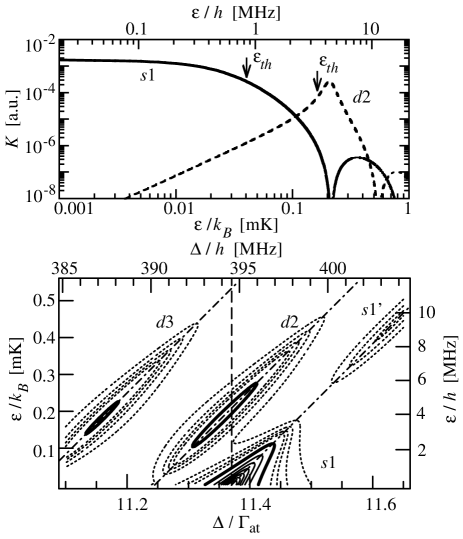
FIG. 3.: The lower panel shows the analytic $K(\varepsilon,\Delta,\ell J)$ in atomic units (1 a.u. $=6.126\times 10^{-9}$ cm${}^{3}/$s) versus $\varepsilon$ and $\Delta$ for $\ell J$ = $s1$, $d2$, and $d3$ ($I=1$ mW/cm²). The vertical and horizontal axes are set to have the same energy scale in common units ($k_{B}/h=$ 20.8 MHz/mK) so that the dash-dot lines of exact resonance, $\varepsilon={\cal E}_{v}(\Delta,J)$, have a 45 degree slant. The dotted contour lines start at 0.000025 and increase in steps of 0.000025. The solid contour lines start at 0.0002 (bold) and increase in steps of 0.0002. The upper panel shows a cut of $K(\varepsilon,\Delta,\ell J)$ for $\ell J=$ $s1$, $d2$ along the dashed vertical line of constant detuning indicated on the lower panel. The analytic threshold range $\varepsilon_{th}$ is indicated.

The variation of $K(\varepsilon,\Delta,\ell J)$ is a consequence of the near-threshold resonance form of $S_{pg}(\varepsilon,\Delta,\ell J)$, Eq. (4). The resonant denominator causes the largest contribution to $K(\varepsilon,\Delta,\ell J)$ to come from energies near the slanted line of exact resonance, $\varepsilon={\cal E}_{v}(\Delta,J)$, indicated in the lower panel of Fig. 3. On the other hand, the term $\Gamma_{vg}(\varepsilon,\ell J)$ [Eq. (5)], proportional to $|\phi_{g}(\varepsilon,\ell,R_{C})|^{2}/k$, is strongly influenced by the near-threshold properties of $\phi_{g}(\varepsilon,\ell,R_{C})$. We may distinguish two regimes: $k\ll k_{th}$ where $|\phi_{g}(\varepsilon,\ell,R_{C})|^{2}/k\propto k^{2\ell}$, and $k\gg k_{th}$, where $|\phi_{g}(\varepsilon,\ell,R_{C})|^{2}/k$ oscillates with an amplitude decreasing as $1/k^{2}\propto 1/\varepsilon$. Thus, the integrand $K(\varepsilon,\Delta,\ell J)$ for $s$-waves approaches a constant value for $k\ll k_{th}$ and drops off rapidly and oscillates when $k\gg k_{th}$. This variation is evident in the upper panel of Fig. 3. Using Eqs. (6) and (7), we estimate $k_{th}$ from $k_{th}|R_{C}-A_{0}|=\pi/2$ for $s$-waves and $k_{th}R_{C}=z_{1}(\ell)$ for $\ell>0$, where the first maximum in $j_{\ell}(z)$ for positive argument is at $z=z_{1}(\ell)$. Taking $R_{C}$ = 513 a₀ and the arbitrary model value $A_{0}=67$ a₀ for our case gives $\varepsilon_{th}/k_{B}=(\hbar k_{th})^{2}/(2\mu k_{B})=$ 0.05 mK for the $s$-wave and 0.18 mK for the $d$-wave. Thus, the large $R_{C}$ leads to the small value for $k_{th}$ and $\varepsilon_{th}$, and consequently to the subthermal linewidth. For energies higher than $\varepsilon_{th}$, $K(\varepsilon,\Delta,\ell J)$ has a node at $\varepsilon$ where $\phi_{g}(\varepsilon,\ell,R_{C})$ has a node at $R_{C}$, e.g., at $\varepsilon/k_{B}=$ 0.21 mK for the $s$-wave and 0.55 mK for the $d$-wave. A second maximum in the ground state wavefunction appears at higher energy, 0.48 mK in the case of the $s$-wave. This is the origin of the maximum in the red wing of the $s1$ feature labeled $s1^{\prime}$ in Figs. 2 and 3.

Figure 4 illustrates the dependence of the $s1$ feature on the unknown ground state scattering length $A_{0}$. Since $k_{th}=\pi/(2|R_{C}-A_{0}|)$, $k_{th}$ decreases for $A_{0}<0$, resulting in narrower thermally averaged lines. However, if $A_{0}$ is positive and near $R_{C}$ so that $|R_{C}-A_{0}|$ becomes small, then $k_{th}$ increases and the narrow peak broadens and flattens, so that it may no longer stand out.

FIG. 4.: Variation of the thermally averaged $s1$ feature at 0.83 mK for three different ground state scattering lengths ($A_{0}=67$ a₀ for Figs. 1-3). Thermal averaging causes the peak to shift from the exact resonance position $\Delta/\Gamma_{\rm at}=11.37$ (where ${\cal E}_{v}=0$) depending on the value of $A_{0}$. The $s1$ feature broadens and shifts considerably when $A_{0}$ becomes close to $R_{C}$. In this case, $\varepsilon_{th}$ increases and a much larger range of collision energies contribute to the thermal average. The feature has a linewidth closer to the natural linewidth of 1.2 MHz and shows more prominent subsidiary maxima when the scattering length is negative. In this case, $\varepsilon_{th}$ decreases and a smaller range of energies contribute to the thermal average.

III Conclusion

We predict that subthermal line shapes should appear in high resolution photoassociation spectra of the ${{}^{1}}\Pi_{g}$ state of Ca dimer near the ¹P$\leftarrow{{}^{1}}$S laser cooling transition. Such features will be hard to see for Mg, where weak ${{}^{1}}\Pi_{g}$ lines are obscured by a large ${{}^{1}}\Sigma_{u}$ background [8]. Subthermal lines may be less prominent for Sr or Ba because of additional predissociation broadening and a higher density of states that combine to give broader and more blended ${{}^{1}}\Pi_{g}$ features.

Subthermal linewidth of scattering resonances are possible when the contributions to the line shape from the relevant $S$-matrix elements is restricted to very low collision energies below the range of thermal energies $k_{B}T$. In our present study, this is a consequence of the very large Condon points associated with the transitions. It would be useful to extend this analysis to other photoassociative transitions or magnetically-induced Feshbach resonances [15]. This would be most interesting in the case of a large $s$-wave scattering length, that is, when $|A_{0}|\gg x_{0}$, where $x_{0}=\frac{1}{2}(2\mu C_{6}/\hbar^{2})^{1/4}$ is a characteristic length scale for a van der Waals potential with dispersion coefficient $C_{6}$ [7]. Since the near threshold range is small, $0<k\ll|A_{0}|^{-1}$, it would be interesting to see if subthermal lineshapes are possible for very narrow resonances with widths $\ll k_{B}T$ when $|A_{0}|$ is large enough that $\hbar^{2}/(2\mu A_{0}^{2})\ll k_{B}T$.

- [1] J. Weiner, V. Bagnato, S. Zilio, and P. S. Julienne, Rev. Mod. Phys. 71, 1 (1999).
- [2] R. Napolitano, J. Weiner, C. J. Williams, and P. S. Julienne, Phys. Rev. Lett. 73, 1352 (1994).
- [3] P. Pillet, A. Crubellier, A. Bleton, O. Dulieu, P. Nosbaum, I. Mourachko, and F. Masnou-Seeuws, J. Phys. B 30, 2801 (1997).
- [4] J. Bohn and P. S. Julienne, Phys. Rev. A 60, 414 (1999).
- [5] K. M. Jones, P. D. Lett, E. Tiesinga, and P. S. Julienne, Phys. Rev. A 61, 012501 (1999).
- [6] J. P. Burke, Jr., C. H. Greene, J. L. Bohn, H. Wang, P. L. Gould, and W. C. Stwalley, Phys. Rev. A 60, 4417 (1999).
- [7] C. J. Williams, E. Tiesinga, P. S. Julienne, H. Wang, W. C. Stwalley, and P. L. Gould, Phys. Rev. A 60, 4427 (1999).
- [8] M. Machholm, P. S. Julienne, and K.-A. Suominen, in press, Phys. Rev. A (2001); LANL preprint, physics/0103059.
- [9] G. Zinner, T. Binnewies, F. Riehle, and E. Tiemann, Phys. Rev. Lett. 85, 2292 (2000).
- [10] W. J. Meath, J. Chem. Phys. 48, 227 (1968).
- [11] This equation, together with Eq. (3), is equivalent to Eq. (22) in Ref. [8], but written in a different form.
- [12] P. S. Julienne, J. Res. Nat. Inst. Stand. Technol. 101, 487 (1996). [http://nvl.nist.gov]
- [13] C. Boisseau, E. Audouard, J. Vigué, and P. S. Julienne, Phys. Rev. A 62, 052705 (2000).
- [14] J. R. Taylor, Scattering Theory (R. E. Krieger, Malabar, 1987).
- [15] V. Vuletić, C. Chin, A. J. Kerman, and S. Chu, Phys. Rev. Lett. 83, 943 (1999).