Rippling patterns in aggregates of myxobacteria
arise from cell-cell collisions

Abstract

Experiments with myxobacterial aggregates reveal standing waves called rippling patterns. Here, these structures are modelled with a simple discrete model based on the interplay between migration and collisions of cells. Head-to-head collisions of cells result in cell reversals. To correctly reproduce the rippling patterns, a refractory phase after each cell reversal has to be assumed, during which further reversal is prohibited. The duration of this phase determines the wavelength and period of the ripple patterns as well as the reversal frequency of single cells.

]

Pattern formation in aggregates of bacteria and amoebae is a widely observed phenomenon[1, 2]. Complex colonial patterns of spots, stripes and rings are produced by E. coli[3]. Bacillus subtilis exhibits branching patterns during colonial growth[4]. Two- and three-dimensional circular waves and spirals have been observed during aggregation of the eukaryotic slime mold Dictyostelium discoideum [5-8], often closely resembling patterns in chemical reactions[9]. These patterns are typically modelled with continuous reaction-diffusion equations describing the spatiotemporal evolution of the cell density and concentrations of chemoattractants and nutrients, e. g. in the cases of Dictyostelium discoideum[1, 10, 11] and E. coli[12, 13]. An alternative approach uses discrete models describing the motion of individual cells and has been previously employed to study swarm behavior [14-16].

The prokaryotic soil bacterium Myxococcus xanthus[17, 18] is one of the most intriguing examples for morphogenesis and pattern formation. Like the slime mold Dictyostelium discoideum, M. xanthus exhibits social behaviour and a complex developmental cycle. As long as there is sufficient food supply, vegetative cells feed on other bacterial species, grow and divide. But when nutrients run short, bacteria start to aggregate and finally build a multicellular structure, the fruiting body. In order to maintain this life cycle intercellular communication is essential. Although a phospholipid chemoattractant has been identified[19] recently, the key role is ascribed to interactions occuring through cell-cell contact during collisions[17].

An experimental example for the rippling phenomenon[20, 21] is displayed in Fig. 1. Bacteria organize into equally spaced ridges (dark regions) that are separated by regions with low cell density (light regions); for a movie see [22]. Rippling patterns were first discovered by one of us (H. Reichenbach) and originally named oscillatory waves. We examine the temporal dynamics of the density profile along a one-dimensional cut indicated by the white line in Fig. 1a. The resulting space-time plot is shown in Fig. 1b and reveals a periodically oscillating standing wave pattern superimposed by spatiotemporal noise.

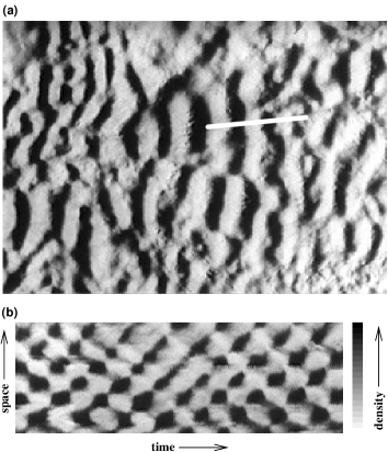
FIG. 1.: (a) Snapshot from a rippling sequence, taken from a time-lapse movie. White bar: 0.5 mm. (b) Space-time plot of the density profile along the white line in (a).

In the following, we present a model based on the dynamics of individual cells for the formation of ripple patterns during the aggregation of myxobacteria. We will show how certain collision rules between cells on the “microscopic” level lead to the observed macroscopic pattern and reproduce the characteristics of single cell behaviour. The basic rules of the model are derived from experimental results by Sager and Kaiser[23]: Within the rippling phase cells are found to move on linear paths parallel to each other about a distance of one wavelength. When two opposite moving cells collide head-on, they reverse their gliding direction due to exchange of a small, membrane-associated protein called C-factor. Furthermore, the model assumes a refractory phase in which cells can not respond to the signal. This additional ingredient is necessary for the formation of the rippling pattern from a random configuration. The characteristic wavelength and period is determined by the duration $\tau$ of the refractory phase. $\tau$ is the only adjustable parameter; the experimental data are reproduced with a refractory period of five minutes.

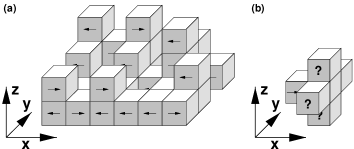
FIG. 2.: (a) Exemplary configuration of the model, the cell orientation is indicated by arrows. (b) The interaction neighborhood is a five nodes cross in the $y,z$-plane at that $x$-position the cell is directed to (here the cell orientation is the $+x$-direction).

In the rippling phase, cells are densely packed and elongated parallel to each other. The organisation of cells into the aligned state can be modeled using particle-based models[15, 16]. Our model is defined on a fixed square grid in the $x-y$-plane and assumes discrete space coordinates, analagous to cellular automaton models. The number of cells in the model is conserved and characterized by the average number $\bar{n}$ of cells per lattice site; cell death and replication of cells are neglected. The discrete $z-$discrete coordinate describes the number of cells piled up on top of each other in a given lattice point in the $x-y$-plane. The temporal update is done in discrete time steps. Cells mainly move along linear paths in the $x$-direction. Thus, even a two-dimensional model is a reasonable first step. Nevertheless, we also study the three-dimensional case because of its experimental relevance. The movement of individual bacteria is restricted to sheets with fixed $y$-coordinate. The coupling in the $y$-direction is solely due to interaction. A single cell is thus described by a three-dimensional space coordinate $(x,y,z)$ and an orientation variable $\phi\in\{-1\mbox{(left)},1\mbox{(right)}\}$ referring to the gliding direction. Cells interact only via head-on collisions, i. e. cells only sense counterpropagating cells in a certain interaction neighborhood.

The sensitivity of a bacterium to C-factor is described by a clock variable $\nu$. When a sensitive cell collides head-on with other cells, (the meaning of collisions will be specified below), it reverses its gliding direction and is refractory for the next $\tau-1$ time steps. $\nu$ measures the time since the last reversal, thus a cell with $\nu<\tau$ is insensitive to C-factor. Overhangs and holes in the bulk are prohibited. A bacterial cell is assumed to cover one node of the lattice, this determines the lattice constants of 10 $\mu$m in $x$- and 1 $\mu$m in $y$- and $z-$directions and the time constant of 1 min.

The temporal update of the model consists of a migration and an interaction step. In the asynchronous migration step cells move according to their orientation to the neighboring site in $x$-direction. If this site is already occupied, the cell pushes its way between cells of the adjacent column increasing its height by 1. With equal probability the cell slips beneath or above the blocking cell. This random process causes internal noise. There is also a diffusion-like noise contribution, because cells are assumed to rest with small probability $p$ (in the simulations below $p=0.05$ is used). Interaction takes place simultaneously; every sensitive cell ($\nu\geq\tau$) checks a neighborhood of five nodes depending on its orientation $\phi$ (Fig. 2b). If a cell encounters at least one cell with opposite orientation in this neighborhood (collision), the cell reverses orientation ($\phi\to-\phi$) and will be refractory for $\tau$ time steps. The cell is insensitive to neighbors but it can still cause the reversal of other cells. Random initial conditions and periodic boundary conditions are used throughout.

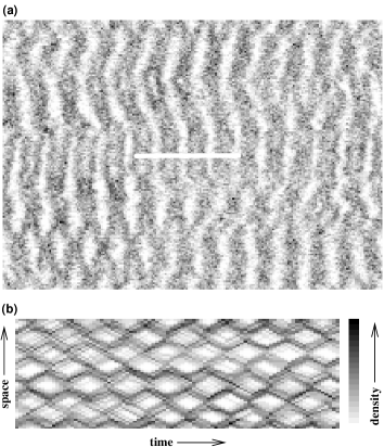
FIG. 3.: (a) Simulation snapshot in a system of size 220$\times$150 with a refractory phase $\tau=5$ (compare to Fig. 1). Typical pattern emerging from random initial conditions after ca. 500 time steps. (b) Space-time plot of the density profile along the white line. The gray scale expresses to the height of the cell column on each site (black corresponds to high columns).

The model described in the previous section reproduces the experimentally observed ripple patterns, see Fig. 3. The rippling pattern and the temporal evolution obtained in the model (Fig. 3) are in good agreement with the experimental data of Fig. 1. Waves propagate equally in both directions, their superposition forms a standing wave. The wavelength of the ripple pattern increases with the duration $\tau$ of the refractory phase. The discrete model enables us to track the single cell behavior. Typically, cells move over a distance of about half a wavelength before they reverse their orientation (see Fig. 4c). The pattern is easily recognizable - wavelength and period of the ripples have been reproduced in several indepedent runs and depend only weakly on the number of cells in the aggregate (variations of the average number $\bar{n}$ of cells per lattice point between 2 and 10 do not produce significant changes, results presented here are for $\bar{n}=3$). Movies of the simulated rippling patterns can be found in [22].

More insight is obtained by deriving a mean-field theory of the discrete model in 2d. Such a description uses a hierarchy of rate equations in discrete time and space, which replace the discrete state variables by their average numbers. The mean-field scheme [24] leads to the following set of $2\tau$ equations:

$$r_{1}(x,t+1) = r_{1}(x-1,t)-f_{r}(x-1,t)+r_{\tau}(x-1,t)$$ (1)

$$r_{2}(x,t+1) = f_{l}(x-1,t)$$ (2)

$$r_{3}(x,t+1) = r_{2}(x-1,t)$$ (3)

$$\vdots$$ (4)

$$r_{\tau}(x,t+1) = r_{\tau-1}(x-1,t)$$ (5)

$$l_{1}(x,t+1) = l_{1}(x+1,t)-f_{l}(x+1,t)+l_{\tau-1}(x+1,t)$$ (6)

$$l_{2}(x,t+1) = f_{r}(x+1,t)$$ (7)

$$l_{3}(x,t+1) = l_{2}(x+1,t)$$ (8)

$$\vdots$$ (9)

$$l_{\tau}(x,t+1) = l_{\tau-1}(x+1,t),$$ (10)

where $r_{1}$ resp. $l_{1}$ are right- resp. left moving cells that can reserve, while $r_{2},...,r_{\tau}$ resp. $l_{2},...,l_{\tau}$ denote right- resp. left moving cells in the various stages of the refractory phase. The functions $f_{r}$ and $f_{l}$ describe the average numbers of reversals of right- resp. left moving cells. The actual form of the reversal function is quite complicated. Since the number of particles on one site is still rather small, it is not sufficient to use their mean values in the reversal function as would be the standard approach for rate equations describing chemical reactions. Instead, one has to specify the distribution of the quantities $l_{1},r_{1}$ around their mean values and sum over all possible states. We have used a Poissonian distribution for this purpose and performed a linear stability analysis of the homogeneous stationary state $r_{1}(x,t)=l_{1}(x,t)=\rho_{S}$ and $r_{i}(x,t)=l_{i}(x,t)=\rho_{R}$ for $i=2,....,\tau$. This state describes a flat layer of cells with equal amounts of left- and right-moving bacteria. The actual values of $\rho_{S}$ and $\rho_{R}$ depend on the parameter $\tau$ and $\bar{n}$ and should obey $\rho_{R}=f_{r}(x,t)=f_{l}(x,t)$ and $\bar{n}=2(\rho_{S}+(\tau-1)\rho_{R})$. For $\tau=5$ and $\bar{n}=3$, we find, for example, $\rho_{S}\approx 0.635$ and $\rho_{R}\approx 0.216$. A detailed derivation of the mean field theory will be published elsewhere [24].

The linear stability analysis of the rate equations (10) with $\bar{n}=3$, reveals a linear instability of this flat layer state against an oscillatory instability with finite wavenumber for $\tau\geq 4$ min [24]. Moreover, we obtain the wavenumber $k$ with the fastest growth rate for $\tau\geq 4$ min resp. weakest damping for $\tau<4$ min and the associated frequency $\omega$ as a function of the refractory time $\tau$. A comparison of the corresponding wavenumber $\lambda=2\pi/k$ and period $T=2\pi/\omega$ with equivalent quantities extracted from a Fourier analysis of simulation data of the discrete model shows good agreement below and near the threshold $\tau\leq 4$ min, see Figs. 4a,b. Above the threshold nonlinear effects lead to a deviation of the predictions from linear stability analysis. It is remarkable that the mode with weakest damping can be observed directly for $\tau\leq 3$ min. It indicates, that the intrinsic noise of the discrete model drives the system out of the linear stable regime and excites the modes with weakest damping.

The wavelength of the pattern in the experiment is about 180 $\mu m$ corresponding to 18 cell lengths. The temporal period in the experiment is found to be around 10 min. Thus, a refractory time $\tau\approx 5$ min in the model yields the correct experimental values for the wavelength as well as for the period. As a third quantity, we can measure the average reversal frequency of the individual cells in the simulations taking advantage of the discrete, particle-based nature of our model. A typical trajectory of an individual cell in the model is displayed in Fig. 4c. Most of the time the cells in the model ride with the ripple crest and get reflected when two crests collide. In other words, while the crest form is seemingly unchanged, most of the cells that originally constituted the crest are now part of a crest propagating in the other direction. Occasionally a cell ,,tunnels” through and continues a longer way with the same crest. For the refractory time $\tau=5$ min, the reversal frequency for a single cell in the model is about 0.15 reversals per cell and minute in the three-dimensional model and 0.1 reversals per cell and minute in two dimensions (see Fig. 4d) which is in the range of the experimentally observed frequency of 0.081 reversals per cell and minute[23].

While previous experiments have not provided direct information about the duration of a refractory phase, recent measurements of reversal rates of myxobacteria exposed to high concentration of isolated C-factor may give a first clue. Sager and Kaiser report an increase of the reversal rate by a factor of 3 compared to normal aggregates and an absolute reversal rate of roughly 0.3 reversals per cell per minute[23]. This suggests a refractory phase between 3 and 4 minutes. The reversal rates from the model with a refractory phase of 5 minutes would increase by a factor of 1.8 for the two-dimensional and by a factor of 1.2 for the three-dimensional model. This small discrepancy between model and experiment may indicate that the refractory time depends on the amount of C-factor and decreases at high concentrations.

We presented a model for the formation of ripple patterns during the aggregation of myxobacteria. The reversal mechanism of cells following collisions has to be supplemented by a refractory phase, that specifies a minimum time between subsequent reversals. The duration of this phase determines the wavelength and the period of the ripple pattern. The ,,microscopic” single cell behavior agrees well with the experiments on the reversal frequency of cells. Our study strongly suggests experiments with single cells to verify the refractory hypothesis and to elucidate its biochemical basis. Moreover, myxobacterial rippling provides the first example of a new mechanism for pattern formation, namely one mediated by migration and direct cell-cell interaction, that may be involved in selforganization processes in other multicellular systems.

FIG. 4.: Ripple wavelength $\lambda$ (a) and period T (b) versus refractory time $\tau$ for 2d simulations (solid squares), 3d simulations (open squares) and 2d mean field theory (solid line). (c) Single cell track with a blow-up of the marked region. d Reversal frequency against refractory time in 2d simulations (solid squares) and 3d simulations (open squares) compared to experiment (dotted line) and largest possible value $r_{\mbox{max}}$ (solid line).

Correspondence and requests for materials should be addressed to M.B. (e-mail: baer@mpipks-dresden.mpg.de).

REFERENCES

- [1] E. Ben-Jacob and H. Levine, Sci. Am. 279, 82 (1998).
- [2] E. Ben Jacob, I. Cohen and H. Levine, Adv. Phys. 49, 395 (2000).
- [3] E. O. Budrene and H. C. Berg, Nature 349, 630 (1991); Nature 376, 49 (1995).
- [4] E. Ben-Jacob et al., Nature 368, 46 (1994).
- [5] G. Gerisch, Naturwissenschaften 58, 430 (1971).
- [6] P. Devreotes, Science 245, 1054 (1989).
- [7] F. Siegert and C. Weijer, J. Cell. Sci 93, 325 (1989); Physica D 49, 224 (1991); Curr. Biol. 5, 937 (1995).
- [8] W. F. Loomis, Microbiol. Rev. 60, 135 (1996).
- [9] R. Kapral and K. Showalter, Eds., Chemical Waves and Patterns (Kluwer, Dordrecht, 1996).
- [10] J. Martiel and A. Goldbeter, Biophys. J. 52, 807 (1987).
- [11] T. Höfer, J. A. Sherratt and P. K. Maini, Proc. Roy. Soc. B 259, 249 (1995).
- [12] L. Tsimring et al., Phys. Rev. Lett. 75, 1859 (1995).
- [13] M. P. Brenner, L. S. Levitov and E. O. Budrene, Biophys. J. 74, 1677 (1998).
- [14] J. K. Parrish and L. Edelstein-Keshet, Science 284, 99 (1999).
- [15] T. Vicsek et al., Phys. Rev. Lett. 75, 1226 (1995).
- [16] H. J. Bussemaker, A. Deutsch and E. Geigant, Phys. Rev. Lett. 78, 5018 (1997).
- [17] M. Dworkin, Microbiol. Rev. 60, 70 (1996).
- [18] L. J. Shimkets, Microbiol. Rev. 54, 473(1990).
- [19] D. B. Kearns and L. J. Shimkets, Proc. Natl. Acad. Sci. U.S.A. 95, 11957 (1998).
- [20] H. Reichenbach, Ber. Deutsch. Bot. Ges. 78, 102 (1965).
- [21] L. J. Shimkets and D. Kaiser, J. Bacteriol. 152, 451 (1982).
-
[22]
Supplementary information:
http://www.mpipksdresden.mpg.de/boerner/supp - [23] B. Sager and D. Kaiser, Genes Dev. 8, 2793 (1994).
- [24] U. Börner, A. Deutsch and M. Bär, in preparation (2001)