Nonlinear equation for curved stationary flames

Abstract

A nonlinear equation describing curved stationary flames with arbitrary gas expansion $\theta=\rho_{{\rm fuel}}/\rho_{{\rm burnt}}$, subject to the Landau-Darrieus instability, is obtained in a closed form without an assumption of weak nonlinearity. It is proved that in the scope of the asymptotic expansion for $\theta\to 1,$ the new equation gives the true solution to the problem of stationary flame propagation with the accuracy of the sixth order in $\theta-1.$ In particular, it reproduces the stationary version of the well-known Sivashinsky equation at the second order corresponding to the approximation of zero vorticity production. At higher orders, the new equation describes influence of the vorticity drift behind the flame front on the front structure. Its asymptotic expansion is carried out explicitly, and the resulting equation is solved analytically at the third order. For arbitrary values of $\theta,$ the highly nonlinear regime of fast flow burning is investigated, for which case a large flame velocity expansion of the nonlinear equation is proposed.

1 Introduction

Curved flame propagation is one of the most important and difficult issues in the combustion theory. Despite considerable efforts, its closed theoretical description is still lacking. Perhaps the main reason underlying complexity of the problem is the intrinsic instability of zero-thickness flames, the Landau-Darrieus (LD) instability [1, 2]. In view of this, evolution of the flame front cannot be prescribed in advance. Instead, it should be determined in the course of joint analysis of the flow dynamics outside the flame front and the heat conduction – species diffusion processes inside. In general, nonlinear interaction of different perturbation modes under the smoothing influence of thermal conduction leads to the formation of a steady curved flame front configuration with the curvature radius of the order $10L_{f},$ where $L_{f}$ is the flame front thickness. This estimate for the curvature radius can be obtained from the linear theory of the LD-instability [3], where it corresponds to the cutoff wavelength for the front perturbations; it is also confirmed by 2D numerical experiments on the flame dynamics [4, 5].

In essential, difficulties encountered in investigation of the nonlinear development of the LD-instability are twofold:

1) Perturbation analysis of the nonlinearity of flame dynamics with arbitrary gas expansion is generally inadequate. In particular, it is completely irrelevant to the problem of formation of the stationary flame configurations.

2) Finite vorticity production in the flame implies that the flow dynamics downstream, and therefore the flame front dynamics itself, is essentially nonlocal. The latter means that the non-locality of equations governing flame propagation is more complex than that encountered in the linear theory and described by the Landau-Darrieus operator.

Only in the case of small gas expansion can the problem be treated both perturbatively and locally, since then the amplitudes of perturbations remain small compared to their wavelengths at all stages of development of the LD-instability [6, 7, 8], and the flow is potential both up- and downstream in the lowest order in $\theta-1,$ where $\theta$ is the ratio of the fuel density and the density of the burnt matter. In this approximation, the nonlinear evolution of the front perturbations is described by the well-known Sivashinsky equation [8].

The nonlinear dynamics of flames with finite gas expansion has been the subject of a number of papers some of which are briefly considered here as the characteristic examples of dealing with the difficulties mentioned above.

To render the problem tractable, certain simplifying assumptions has been introduced by various authors in attempt to weaken or even get rid of one of the two above features inherent to the nonlinear flame dynamics. In Ref. [9], the vorticity production in the flame is completely neglected [see the point 2) above]. The mass conservation and the constant normal flame velocity are taken as the conditions governing flame dynamics. The problem is reduced thereby to the well-known electrodynamic problem of determining the single layer potential with constant charge distribution proportional to the gas expansion. However, neglecting the vorticity downstream breaks the continuity of tangential velocity components as well as the constant jump of pressure across the flame. This model thus violates the basic conservation laws to be satisfied across the flame front. Note that the number of neglected degrees of freedom (three in the 3-dimensional case) just corresponds to the number of broken conservation laws (two tangential velocity components and the scalar pressure).

In contrast, in Ref. [10], an attempt is made to take into account the vorticity production in stationary flames, under the assumption of weak nonlinearity [see the point 1) above]. From the mathematical point of view, however, the assumptions of weak nonlinearity and stationarity contradict each other. Using them simultaneously turns out to be inconsistent except for the case of small gas expansion. Indeed, let us consider a weakly curved flame front propagating in $z$-direction with unit normal velocity with respect to an initially uniform fuel; the transverse coordinates will be denoted x. It is not difficult to show that in this case the flow equations up- and downstream together with the conservation laws at the flame front imply the following relation between the flame front position, $z=f({\bf x},t)-t,$ and $z$-component of the fuel velocity ${\bf v}={\bf v}({\bf x},z,t)$ just ahead of the front, $u_{-}={\rm v}_{z}({\bf x},f({\bf x},t)-0,t),$

$$u_{-}+\frac{\theta+1}{2\theta}\hat{\Phi}^{-1}\frac{\partial u_{-}}{\partial t}=\frac{\theta-1}{2}\hat{\Phi}f,$$ (1)

where $\hat{\Phi}$ denotes the Landau-Darrieus operator defined by

$$(\hat{\Phi}f)({\bf x})=\int_{-\infty}^{+\infty}d{\bf k}|{\bf k}|f_{\bf k}\exp(i{\bf kx}),$$

$f_{\bf k}$ being the Fourier transform of $f.$ (It is assumed here that ${\bf v}(z=-\infty)=0$ in the laboratory frame of reference. Details can be found, e.g., in Ref. [11]) On the other hand, to the leading order in the front slope $\partial f/\partial{\bf x},$ the condition of unit normal flame velocity with respect to the fuel gives

$$u_{-}\ =\frac{\partial f}{\partial t}+\frac{1}{2}\left(\frac{\partial f}{\partial{\bf x}}\right)^{2}.$$ (2)

In the regime of steady flame propagation,

$$\frac{\partial u_{-}}{\partial t}=0,~{}~{}\frac{\partial f}{\partial t}=-W,$$

where $W\sim(\partial f/\partial{\bf x})^{2}$ is the flame velocity increase due to the front curvature. Substituting this into relations (1), (2) gives

$$-W+\frac{1}{2}\left(\frac{\partial f}{\partial{\bf x}}\right)^{2}=\frac{\theta-1}{2}\hat{\Phi}f.$$ (3)

Since the right hand side of this equation is linear in the slope, while the left hand side is only quadratic, nonlinearity can be considered small only if $\theta-1$ is small, in which case one has $\partial f/\partial{\bf x}\sim\theta-1,$ $W\sim(\theta-1)^{2}.$ Thus, for arbitrary $\theta,$ the weak nonlinearity approach to the stationary flames, advocated in [10], turns out to be self-contradictory. From the physical point of view, this means that a weakly curved flame with finite gas expansion cannot be stationary. Instead, equations (1), (2) should be considered in this case as determining evolution of the small perturbations in time. Indeed, substituting Eq. (2) into Eq. (1), we obtain, in the linear approximation,

$$\frac{\theta+1}{2\theta}\hat{\Phi}^{-1}\frac{\partial^{2}f}{\partial t^{2}}+\frac{\partial f}{\partial t}-\frac{\theta-1}{2}\hat{\Phi}f=0,$$ (4)

which is nothing but the well-known LD dispersion relation for the perturbation growth rate, written in the coordinate space [1, 2].

In practice, the discrepancy in the orders of magnitude, expressed by Eq. (3), shows itself as the impossibility to correctly develop perturbation expansion in powers of the slope. For instance, the jump of the pressure field across the flame front, found in Ref. [10], Eq. (33), turns out to be velocity-dependent already for zero thickness flames, while according to the well-known exact result [12] this jump is constant along the flame front, and is equal to $1-\theta.$

It should be stressed that the above-mentioned inconsistency resides in the equations of motion themselves; it is inherent, therefore, to the flame propagation in tubes as well as to unbounded flames. Indeed, even in the case of very narrow tubes, numerical experiments on flames with $\theta=6~{}\div~{}8$ give values of about $1.5~{}\div~{}2.0$ for the slope [5].

Finally, we mention Ref. [13], where a non-stationary equation describing the interaction of perturbations at the early stage of development of LD instability is obtained at the second order of nonlinearity, under a certain model assumption concerning the structure of downstream flow. Namely, it is assumed that there exists a local relation between the pressure field and the potential mode of the velocity downstream (expressed by the Bernoulli equation). However, as we mentioned in 2), the flow dynamics downstream is essentially nonlocal, in particular, the pressure field is expressed through the velocity field by an integral relation, its kernel being an appropriate Green function of the Laplace operator. From the work [13], one can see once again that the perturbative treatment of nonlinearities is not applicable to the stationary flames with arbitrary $\theta:$ since, at the first order, the time derivatives of the front position are linearly related to its space derivatives through Eq. (4), stationary form of the non-stationary Zhdanov-Trubnikov equation depends on the way this relation is used before the time derivatives are omitted. Transition to the stationary regime in this equation is therefore ambiguous.

In view of what has been said, we arrive at the conclusion that the stationary flames can only be treated consistently in the framework of the small $\theta-1$ expansion. Thus, the problem of describing the stationary flames, and more generally, non-stationary flames in the fully developed nonlinear regime, can be formulated as the problem of deriving an expansion of unknown exact equation, governing flame dynamics, in powers of $\theta-1.$

The purpose of the present paper is to show that in the stationary case, such an expansion can indeed be developed beyond the second order, the order of validity of the Sivashinsky equation. We found it convenient to employ the model assumption of Ref. [13] in our analysis, which allows one to obtain an equation describing flames with arbitrary gas expansion in a closed form, without the assumption of weak nonlinearity. This will be shown in Sec. 3.1 on the basis of simple geometric considerations. That the equation obtained actually provides the true expansion of (unknown) exact equation with the accuracy of the sixth(!) order in $\theta-1$ is proved in Sec. 3.2. This expansion is carried out explicitly in Sec. 4.1. The third order equation turns out to have the functional structure analogous to the Sivashinsky equation, and therefore can be solved analytically. This solution is found in Sec. 4.2. Finally, the model equation obtained in Sec. 3.1 is invoked in Sec. 5 for investigation of the highly nonlinear regime of fast flow burning, where a large flame velocity expansion of this equation is proposed. The results of the present work are summarized in Sec. 6. Some mathematical results used in the text are derived in the Appendix.

2 Flow equations and conservation laws

Let us consider a 2D flame propagating in an initially uniform premixed fluid. Since our main concern is the influence of finite gas expansion on the flame structure, we will assume in what follows that the fluid is an ideal gas with constant thermal conduction and constant specific heat. The ratio of the heat and mass diffusivities (the Lewis number) is taken to be unity. For definiteness, we consider flame propagation in a tube of arbitrary width with ideally slip adiabatic walls. Under the assumption that development of the LD instability ends up with the formation of a steady flame configuration, we go over to the reference frame of the stationary flame. Let the Cartesian coordinates $(x,z)$ be chosen so that $z$-axis is parallel to the tube walls, $z=-\infty$ being in the fresh fuel. It will be convenient to introduce the following dimensionless variables

$$(\eta;\xi)=(x/R;z/R),\ (w;u)=({\rm v}_{x}/U_{f};{\rm v}_{z}/U_{f}),$$

$$\Pi=(P-{P}_{f})/{\rho}_{-}{U_{f}}^{2},$$

where $U_{f}$ is the velocity of a plane flame front, $P_{f}$ is the initial pressure in the fuel far ahead of the flame front, and $R$ is some characteristic length of the problem (e.g., the cut-off wavelength). The fluid density will be normalized on the fuel density $\rho_{-}.$ As always, we assume that the process of flame propagation is nearly isobaric. Then the velocity and pressure fields obey the following equations in the bulk

$$\frac{\partial u}{\partial\xi}+\frac{\partial w}{\partial\eta}=0,$$ (5)

$$u\frac{\partial u}{\partial\xi}+w\frac{\partial u}{\partial\eta}=-\frac{1}{\rho}\frac{\partial\Pi}{\partial\xi},$$ (6)

$$u\frac{\partial w}{\partial\xi}+w\frac{\partial w}{\partial\eta}=-\frac{1}{\rho}\frac{\partial\Pi}{\partial\eta}.$$ (7)

The above flow equations are complemented by the following conservation laws to be satisfied across the flame front

$$u_{+}-\theta u_{-}-f^{\prime}(w_{+}-\theta w_{-})=0,$$ (8)

$$w_{+}-w_{-}+f^{\prime}(u_{+}-u_{-})=0,$$ (9)

$$\Pi_{+}-\Pi_{-}=-(\theta-1),$$ (10)

where the flame front position is given by $\xi=f(\eta),$ the subscripts ”$+$” and ”$-$” mean that the corresponding quantity should be evaluated at $\xi=f(\eta)+0$ and $\xi=f(\eta)-0,$ respectively, and

$$N\equiv\sqrt{1+f^{\prime 2}},~{}~{}f^{\prime}\equiv\frac{df}{d\eta}.$$

Finally, the normal velocity of the fuel at the flame front is unity, which is expressed in the form of the evolution equation

$$u_{-}-f^{\prime}w_{-}=N.$$ (11)

Equations (8)–(11) are written for zero thickness flames. These are of primary interest, since in the majority of cases the thickness of the flame front is small compared with the fluid-dynamical scale of the problem. Formal generalization to the case of small but nonzero thickness is straightforward and will be done in Sec. 3.3.

In principle, the system of equations (5) – (11) completely determines stationary flame configuration as well as the flows upstream and downstream. To derive an equation for the flame front function $f(\eta),$ one has to find solution of the bulk equations (5) – (7) for the fuel and combustion products with appropriate boundary conditions on the walls, subject to the conservation laws (8) – (10) which are a kind of boundary conditions on the flame front. The requirement that the obtained solution satisfies Eq. (11) then gives an equation for the function $f(\eta)$ itself.

As to the flow upstream, the corresponding solution is readily obtained: since the flow is potential at $\xi=-\infty$ ($u=V,$ $w=0,$ where $V$ is the velocity of the flame in the rest frame of reference of the fuel), it is potential for every $\xi<f(\eta)$ in view of the Helmholtz theorem [14], thus

$$u\equiv V+\tilde{u}=V+\int\limits_{-\infty}^{+\infty}dk~{}\tilde{u}_{k}\exp(|k|\xi+ik\eta),$$ (12)

$$w=\hat{H}\tilde{u},$$ (13)

$$\Pi+\frac{1}{2}(u^{2}+w^{2})={\rm const_{1}},$$ (14)

where the Hilbert operator

$$(\hat{H}f)(\eta)=\frac{1}{\pi}{\rm p.v.}\int\limits_{-\infty}^{+\infty}d\zeta\frac{f(\zeta)}{\zeta-\eta},$$

”${\rm p.v.}$” denoting the principal value. Although the relation $w=\hat{H}\tilde{u}$ between the velocity components upstream is nonlocal, it is expressed in terms of the transverse coordinate $\eta$ only.

Things become more complicated downstream. There, no relation exists for the variables $u,~{}w,~{}\Pi,$ which can be expressed in terms of $\eta$ alone, since the $\xi$-dependence of these variables is unknown because of the presence of vorticity produced by the curved flame. Nevertheless, we will assume following Ref. [13] that a potential mode ${\bf v}_{p}=(w_{p},u_{p})$ can be extracted from the downstream velocity ${\bf v}=(w,u),$ such that the following Bernoulli-type relation holds between ${\bf v}_{p}$ and $\Pi$

$$\Pi+\frac{1}{2\theta}(u_{p}^{2}+w_{p}^{2})={\rm const_{2}}.$$ (15)

Then Eqs. (5) – (7) can be rewritten as

$$\frac{\partial u}{\partial\xi}+\frac{\partial w}{\partial\eta}=0,~{}~{}\frac{\partial u_{p}}{\partial\xi}+\frac{\partial w_{p}}{\partial\eta}=0,$$ (16)

$$u\frac{\partial u}{\partial\xi}+w\frac{\partial u}{\partial\eta}-u_{p}\frac{\partial u_{p}}{\partial\xi}-w_{p}\frac{\partial u_{p}}{\partial\eta}=0,$$ (17)

$$u\frac{\partial w}{\partial\xi}+w\frac{\partial w}{\partial\eta}-u_{p}\frac{\partial w_{p}}{\partial\xi}-w_{p}\frac{\partial w_{p}}{\partial\eta}=0.$$ (18)

The general solution for the potential mode can be written analogously to Eqs. (12), (13)

$$u_{p}\equiv\theta V+\tilde{u}_{p}=\theta V+\int\limits_{-\infty}^{+\infty}dk~{}\tilde{u}_{k}\exp(-|k|\xi+ik\eta),$$ (19)

$$w_{p}=-\hat{H}\tilde{u}_{p}.$$ (20)

The model relation (15) does not uniquely define the potential mode, since a constant term in the $\xi$-component of the velocity can be assigned either to the potential mode or to the vorticity mode. As will be shown in Sec. 3.2, the vorticity produced in a flame is only of the fourth order in $(\theta-1)$ as $\theta\to 1.$ The choice $\theta V$ of the constant term in Eq. (19) is fixed therefore up to the second order by the requirement that the mass flow at $\xi=+\infty,$ where $u=u_{p}={\rm const},w=0,$ equals that at $\xi=-\infty$.

Now, using the continuity equations (16) for ${\bf v}$ and ${\bf v}_{p},$ Eq. (17) can be written in the form in which $\xi$-dependence is implicit

$$u\frac{\partial w}{\partial\eta}-w\frac{\partial u}{\partial\eta}-u_{p}\frac{\partial w_{p}}{\partial\eta}+w_{p}\frac{\partial u_{p}}{\partial\eta}=0.$$ (21)

It will be shown in the next section, the above equations for the potential mode upstream and downstream, equation (21), and the conservation laws at the flame front constitute the system of equations sufficient to derive an equation for the function $f(\eta)$ in a closed form.

3 Nonlinear equation for the flame front

3.1 Derivation

It will be shown presently that the set of equations (8) – (11), (13) – (15), (20), and (21) can be transformed into one equation for the function $f(\eta).$ The fact that this set is written in a form that does not explicitly operates with the $\xi$-dependence of the flow variables makes it unnecessary to follow the program outlined in the preceding section to obtain an equation for $f(\eta).$ Namely, the specific structure of the up- and downstream flows in the bulk is now irrelevant. In particular, knowledge of the $\xi$-dependence of the velocity and pressure fields turns out to be superfluous. Roughly speaking, the $\xi$-dependence of a function $F(\xi,\eta)$ describing the shape of the flame front is known in advance, since the equation $F(\xi,\eta)=0$ can always be brought into the form $\xi-f(\eta)=0$ (with $f$ many-valued, in general). Determination of the $\eta$-dependence alone of the functions involved is therefore sufficient for the purpose of description of the flame front structure.

In what follows, it will be convenient to introduce separate designations for the up- and downstream velocity and pressure fields. Namely, they will be distinguished by the superscripts $"+"$ and $"-"$, respectively. Then, setting $\xi=f(\eta),$ equations (13), (14), (15), (20), and (21), together with the conservation laws (8) – (10) and the evolution equation (11), can be rewritten identically as follows

$$\left(\begin{array}[]{rcc}u^{+}-\theta u^{-}-f^{\prime}(w^{+}-\theta w^{-})&=&0\\ w^{+}-w^{-}+f^{\prime}(u^{+}-u^{-})&=&0\\ \Pi^{+}-\Pi^{-}&=&-(\theta-1)\\ u^{-}-f^{\prime}w^{-}&=&N\\ w^{-}&=&\hat{H}\tilde{u}^{-}\\ \Pi^{-}+\frac{1}{2}\{(u^{-})^{2}+(w^{-})^{2}\}&=&{\rm const_{1}}\\ \Pi^{+}+\frac{1}{2\theta}\{(u_{p}^{+})^{2}+(w_{p}^{+})^{2}\}&=&{\rm const_{2}}\\ w_{p}^{+}&=&-\hat{H}\tilde{u}_{p}^{+}\\ u^{+}\frac{\partial w^{+}}{\partial\eta}-w^{+}\frac{\partial u^{+}}{\partial\eta}-u_{p}^{+}\frac{\partial w_{p}^{+}}{\partial\eta}+w_{p}^{+}\frac{\partial u_{p}^{+}}{\partial\eta}&=&0\end{array}\right)_{\xi=f(\eta)}$$

Suppose we have found a solution $f=f(\eta),$ ${\bf v}^{-}={\bf v}^{-}(\xi,\eta),$ ${\bf v}^{+}={\bf v}^{+}(\xi,\eta),$ etc. of the set of equations in the large brackets in ($*$). Then, in particular, these equations are satisfied for $\xi=f(\eta).$ On the other hand, since no operation involving $\xi$ appears in these equations, the function $f(\eta)$ is one and the same for all solutions. Furthermore, since $f(\eta)$ is $\xi$-independent, it is convenient to work with the particular solution in which all the other functions are also $\xi$-independent, and to omit the large brackets in ($*$). Therefore, we replace the above set of equations by the following

$$\upsilon^{+}-\theta\upsilon^{-}-f^{\prime}(\omega^{+}-\theta\omega^{-}) = 0$$ (22)

$$\omega^{+}-\omega^{-}+f^{\prime}(\upsilon^{+}-\upsilon^{-}) = 0$$ (23)

$$\pi^{+}-\pi^{-} = -(\theta-1)$$ (24)

$$\upsilon^{-}-f^{\prime}\omega^{-} = N$$ (25)

$$\omega^{-} = \hat{H}\tilde{\upsilon}^{-}$$ (26)

$$\pi^{-}+\frac{1}{2}\{(\upsilon^{-})^{2}+(\omega^{-})^{2}\} = {\rm const_{1}}$$ (27)

$$\pi^{+}+\frac{1}{2\theta}\{(\upsilon_{p}^{+})^{2}+(\omega_{p}^{+})^{2}\} = {\rm const_{2}}$$ (28)

$$\omega_{p}^{+} = -\hat{H}\tilde{\upsilon}_{p}^{+}$$ (29)

$$\upsilon^{+}\frac{d\omega^{+}}{d\eta}-\omega^{+}\frac{d\upsilon^{+}}{d\eta}-\upsilon_{p}^{+}\frac{d\omega_{p}^{+}}{d\eta}+\omega_{p}^{+}\frac{d\upsilon_{p}^{+}}{d\eta} = 0,$$ (30)

where $\upsilon,\omega,$ and $\pi$ are the $\xi$-independent counterparts of the flow variables $u,w,$ and $\Pi,$ respectively, and

$$\upsilon^{-}\equiv V+\tilde{\upsilon}^{-},~{}~{}\upsilon_{p}^{+}\equiv\theta V+\tilde{\upsilon}_{p}^{+}.$$ (31)

The fact that now the function $f(\eta)$ does not enter the arguments of these variables allows us to avoid expanding them in powers of $f$ (employed, e.g., in Refs. [13, 10]). In fact, such an expansion is irrelevant to the issue whatever regime (stationary or not) is considered, since all the equations governing flame propagation are invariant with respect to the space translations, and therefore, all terms containing powers of undifferentiated $f$ should appear in invariant combinations in the final equation for $f.$ On the other hand, in view of the above-mentioned translation invariance, the function $f$ itself does not need to be small even if the front is only weakly curved (e.g., at the early stage of development of the LD-instability). We thus see that the $f$-dependence of the flow variables through their arguments must eventually cancel in some way.

Let us now turn to the derivation of the equation for the function $f(\eta).$

From the geometric point of view, Eqs. (24), (27), (28) determine the amplitude $\Omega$ of the complex function

$$\upsilon^{+}_{p}+i\omega^{+}_{p}\equiv\Omega e^{i\phi},$$ (32)

while Eq. (30) gives the rate of change of its phase $\phi$ along the flame front. Indeed, Eq. (30) can be rewritten as

$$\frac{d\phi}{d\eta}=\frac{\upsilon^{+}d\omega^{+}/d\eta-\omega^{+}d\upsilon^{+}/d\eta}{(\upsilon_{p}^{+})^{2}+(\omega_{p}^{+})^{2}}.$$ (33)

Then Eqs. (22), (23), (25), and (26) allow one to express the right hand side of Eq. (33) in terms of the function $f(\eta),$ while Eq. (29) plays the role of the consistency condition which gives the equation for the function $f(\eta)$ itself.

Specifically, Eqs. (24), (27), and (28) imply that

$$\Omega^{2}=(\upsilon_{p}^{+})^{2}+(\omega_{p}^{+})^{2}=\theta\{(\upsilon^{-})^{2}+(\omega^{-})^{2}\}+C,$$ (34)

with some constant $C.$ As in Eq. (19) above, this constant is fixed up to the second order in $\theta-1,$ since to this order the flow is potential downstream, $\upsilon^{+}=\upsilon_{p}^{+},$ $\omega^{+}=\omega_{p}^{+}.$ The actual value of $C$ can be found calculating Eq. (34) at some particular point at the flame front. At the tube walls, e.g., one has $\upsilon^{-}=1,$ $\upsilon^{+}=\theta,$ $\omega^{-}=\omega^{+}=0,$ therefore,

$$C=\theta(\theta-1).$$ (35)

We will see in Sec. 5 that from the point of view of the large flame velocity expansion, another choice of the constant $C$ is more appropriate: $C=\theta(\theta-1)V^{2}.$ This differs from that of Eq. (35) only in the third order in $\theta-1,$ since $V=1+O((\theta-1)^{2})$ (see Sec. 3.2 below).

Next, solving Eqs. (22), (23) with respect to $\upsilon^{+},$ $\omega^{+},$ and using Eqs. (34), (35), we derive the following expression for the phase derivative

$$\phi^{\prime}=\frac{\left(V+\tilde{\upsilon}^{-}+\frac{\theta-1}{N}\right)\left(\hat{H}\tilde{\upsilon}^{-}-f^{\prime}\frac{\theta-1}{N}\right)^{\prime}-\left(\hat{H}\tilde{\upsilon}^{-}-f^{\prime}\frac{\theta-1}{N}\right)\left(\tilde{\upsilon}^{-}+\frac{\theta-1}{N}\right)^{\prime}}{\theta\left[(V+\tilde{\upsilon}^{-})^{2}+(\hat{H}\tilde{\upsilon}^{-})^{2}+(\theta-1)\right]}.$$ (36)

Eqs. (25) and (26) imply that the function $\tilde{\upsilon}^{-}=\tilde{\upsilon}^{-}(\eta)$ entering this equation can be represented in terms of $f(\eta)$ by formally inverting the operator $(1-f^{\prime}\hat{H}):$

$$\tilde{\upsilon}^{-}=(1-f^{\prime}\hat{H})^{-1}(N-V).$$ (37)

The right hand side of this equation can be represented as a formal series in powers of the operator $f^{\prime}\hat{H}:$

$$(1-f^{\prime}\hat{H})^{-1}(N-V)=(1+f^{\prime}\hat{H}+f^{\prime}\hat{H}f^{\prime}\hat{H}+\cdot\cdot\cdot)(N-V).$$

Now, to obtain the equation for $f(\eta),$ we have to use the remaining equation (29). In terms of the quantities $\Omega$ and $\phi,$ it takes the form

$$({\rm Im}+{\rm Re}\hat{H})(\Omega e^{i\phi}-\theta V)=0,$$ (38)

where ${\rm Re}F$ and ${\rm Im}F$ denote the real and imaginary parts of the complex function $F,$ respectively, and we used the fact that the Hilbert operator is real (see the Appendix). To combine Eqs. (34), (36), and (38) into one, one has to solve the latter with respect to $\phi.$ This can be done as follows.

Noting the relations ${\rm Im}iF={\rm Re}F,$ ${\rm Re}iF=-{\rm Im}F,$ we can rewrite Eq. (38) identically as

$${\rm Im}(1+i\hat{H})(\Omega e^{i\phi}-\theta V)=0,$$ (39)

or as

$${\rm Re}(i-\hat{H})(\Omega e^{i\phi}-\theta V)=0.$$ (40)

Acting by the operator $\hat{H}$ on Eq. (40) from the left, and using the identity (94) of the Appendix, this equation can be rewritten also as

$${\rm Re}(i\hat{H}+1)(\Omega e^{i\phi}-\theta V)=0.$$ (41)

Together, Eqs. (39) and (41) imply that

$$(1+i\hat{H})(\Omega e^{i\phi}-\theta V)=0.$$ (42)

Let us consider the structure of Eq. (42) more closely.

Lemma: All solutions of the equation

$$(1+i\hat{H})X=0$$ (43)

span the ring.

Proof: First, let us show that if $X$ is a solution of Eq. (43), then its square $X^{2}$ also is. Indeed, using the identity (98) of the Appendix, one has

$$2i\hat{H}X^{2}=2\hat{H}(X\hat{H}X)=(\hat{H}X)^{2}-X^{2}=-X^{2}-X^{2},$$

therefore,

$$(1+i\hat{H})X^{2}=0.$$

In view of the linearity of the Hilbert operator, the sum $X_{1}+X_{2}$ of two solutions $X_{1},$ $X_{2}$ of Eq. (43) also is a solution,

$$(1+i\hat{H})(X_{1}+X_{2})=0,$$ (44)

and so are the squares $X_{1}^{2},$ $X_{2}^{2},$ and $(X_{1}+X_{2})^{2},$ as we just proved. We have, therefore,

$$0=(1+i\hat{H})(X_{1}+X_{2})^{2}=(1+i\hat{H})(X_{1}^{2}+2X_{1}X_{2}+X_{2}^{2})=2(1+i\hat{H})(X_{1}X_{2}),$$

or

$$(1+i\hat{H})(X_{1}X_{2})=0.$$ (45)

In particular, it follows from Eq. (45) by induction that for any solution $X$ of Eq. (43) and any positive integer $n,$

$$(1+i\hat{H})X^{n}=0,~{}n\in N.$$

In mathematical terminology, the properties (44) and (45) reveal the ring structure of solutions of Eq. (43).

This result can be used to solve Eq. (42) with respect to $\phi.$ Namely, assuming that $|\Omega e^{i\phi}/\theta V-1|<1,$ and taking the infinite sum of the powers

$$\left(\frac{\Omega e^{i\phi}}{\theta V}-1\right)^{n}$$

multiplied by the factors $\frac{1}{n},$ we obtain

$$(1+i\hat{H})\sum\limits_{n=1}^{\infty}\frac{1}{n}\left(\frac{\Omega e^{i\phi}}{\theta V}-1\right)^{n}=(1+i\hat{H})\ln\left\{1+\left(\frac{\Omega e^{i\phi}}{\theta V}-1\right)\right\}$$

$$=(1+i\hat{H})\left(\ln\frac{\Omega}{\theta V}+i\phi\right)=0,$$ (46)

or

$$\phi=-\hat{H}\ln\frac{\Omega}{\theta V}.$$ (47)

This solution is then analytically continued for all values of $\Omega,$ $\phi.$

With the help of Eqs. (34) – (36), and (47) we can now write the equation for the function $f(\eta)$ we are looking for

$$\frac{\theta}{2}\frac{d}{d\eta}\ln\left\{(V+\upsilon)^{2}+(\hat{H}\upsilon)^{2}+(\theta-1)\right\}$$

$$=\hat{H}\left\{\frac{\left(V+\upsilon+\frac{\theta-1}{N}\right)\left(\hat{H}\upsilon-f^{\prime}\frac{\theta-1}{N}\right)^{\prime}-\left(\hat{H}\upsilon-f^{\prime}\frac{\theta-1}{N}\right)\left(\upsilon+\frac{\theta-1}{N}\right)^{\prime}}{(V+\upsilon)^{2}+(\hat{H}\upsilon)^{2}+(\theta-1)}\right\},$$ (48)

with the denotation

$$\upsilon\equiv(1-f^{\prime}\hat{H})^{-1}(N-V).$$ (49)

Before we proceed to the investigation of this equation, let us consider the question of its accuracy.

3.2 Accuracy assessment

We derived Eq. (3.1) using only exact transformations of the equations (22) – (30). Therefore, its accuracy is determined entirely by the accuracy of the underlying model assumption expressed by Eq. (15), which can be estimated as follows.

As we have mentioned above, the exact equation for the stationary flame front can, in principle, be obtained from the system of equations (5) – (11), of which only the $\eta$-component of the Euler equations, Eq. (7), is not present in the set ($*$) of equations describing our model. The question of the model accuracy, therefore, is the question of the accuracy to which Eq. (7) is satisfyed by the model solution. To answer the latter, we need an explicit expression for the vorticity produced in the flame, which will be derived presently.

It was shown in Ref. [12] that with the help of the conservation laws (8) – (10) and the evolution equation (11), the value of the vorticity just behind the flame front can be explicitly expressed in terms of the fuel velocity. Namely, with the help of Eqs. (5.32) and (6.15) of the work [12], the jump $\{\sigma\}_{-}^{+}$ of the vorticity

$$\sigma=\frac{\partial u}{\partial\eta}-\frac{\partial w}{\partial\xi}$$

across the flame front can be written, in the 2D stationary case, as

$$\{\sigma\}_{-}^{+}=-\frac{\theta-1}{\theta N}\left(\hat{D}w_{-}+f^{\prime}\hat{D}u_{-}+\frac{1}{N}\hat{D}f^{\prime}\right),$$ (50)

where

$$\hat{D}\equiv\left(w_{-}+\frac{f^{\prime}}{N}\right)\frac{d}{d\eta}.$$ (51)

Differentiating the evolution equation (11) and writing Eq. (50) longhand, expression in the brackets can be represented as a total derivative

$$\hat{D}w_{-}+f^{\prime}\hat{D}u_{-}+\frac{1}{N}\hat{D}f^{\prime}\equiv w_{-}^{\prime}w_{-}+\frac{(f^{\prime}w_{-})^{\prime}}{N}+\frac{(f^{\prime})^{2}u_{-}^{\prime}}{N}+f^{\prime}u_{-}^{\prime}w_{-}+\frac{N^{\prime}}{N}$$

$$=\frac{(w_{-}^{2})^{\prime}}{2}+\frac{(u_{-}-N)^{\prime}}{N}+\frac{(N^{2}-1)u_{-}^{\prime}}{N}+u_{-}^{\prime}(u_{-}-N)+\frac{N^{\prime}}{N}=\frac{(u_{-}^{2}+w_{-}^{2})^{\prime}}{2}.$$ (52)

Since the flow is potential upstream, we obtain the following expression for the vorticity just behind the flame front

$$\sigma_{+}=-\frac{\theta-1}{2\theta N}(u_{-}^{2}+w_{-}^{2})^{\prime}.$$ (53)

With the help of this equation, we can now show that Eq. (7) is actually satisfied by the model solution with the accuracy of the sixth order in $\alpha\equiv\theta-1,$ as $\alpha\to 0.$

First of all, the following estimates can be readily obtained [8]:

$$f^{\prime}=O(\alpha),~{}~{}~{}\tilde{u},w\sim(f^{\prime})^{2}=O(\alpha^{2}),$$

and, more generally,

$$\frac{dF}{d\eta}=O(\alpha)O(F),$$

for any functional $F=F[f(\eta)],$ since the amplitude $A$ of a perturbation of the flame front with the wavelength $\lambda$ is of the order $\alpha\lambda$ [6, 7, 8]. In particular, it follows from Eq. (53) that

$$\sigma=O(\alpha^{4}).$$ (54)

Next, we rewrite Eq. (7) identically

$$u\frac{\partial u}{\partial\eta}+w\frac{\partial w}{\partial\eta}-u\sigma=-\frac{1}{\rho}\frac{\partial\Pi}{\partial\eta}.$$ (55)

Setting $\xi=f(\eta)+0$ in this equation and using Eq. (53), we obtain

$$\left(\frac{\partial}{\partial\eta}\frac{u^{2}+w^{2}}{2}\right)_{+}+u_{+}\frac{\theta-1}{2\theta N}\frac{d}{d\eta}(u_{-}^{2}+w_{-}^{2})=-\theta\left(\frac{\partial\Pi}{\partial\eta}\right)_{+}.$$ (56)

Using the above estimates and taking into account that $u_{+}=\theta V+\tilde{u}_{+},$ $V=1+O(\alpha^{2}),$ Eq. (56) can be rewritten as

$$\left(\frac{\partial}{\partial\eta}\frac{u^{2}+w^{2}}{2}\right)_{+}+(\theta-1)\frac{d}{d\eta}\frac{u_{-}^{2}+w_{-}^{2}}{2}=-\theta\left(\frac{\partial\Pi}{\partial\eta}\right)_{+}+O(\alpha^{6}).$$ (57)

On the other hand, similar transformations of Eq. (6) give, with the same accuracy,

$$\left(\frac{\partial}{\partial\xi}\frac{u^{2}+w^{2}}{2}\right)_{+}=-\theta\left(\frac{\partial\Pi}{\partial\xi}\right)_{+}+O(\alpha^{6}).$$ (58)

Finally, taking the sum of Eq. (57) and Eq. (58) multiplied by $f^{\prime},$ and noting that

$$u_{+}^{2}+w_{+}^{2}=u_{-}^{2}+w_{-}^{2}+\theta^{2}-1,~{}~{}\Pi_{+}=\Pi_{-}-(\theta-1),$$

we get

$$\frac{d}{d\eta}\left\{\frac{1}{2}\left(u_{-}^{2}+w_{-}^{2}\right)+\Pi_{-}\right\}=O(\alpha^{6}).$$ (59)

Since the flow is potential upstream, the left hand side of Eq. (59) is zero. We conclude that Eq. (59), and therefore Eq. (7), is satisfied with the accuracy of the sixth order in $\alpha.$

It is worth to emphasize that the model equation (15) has not been used in the derivation of Eq. (59). Therefore, the latter holds true whatever model is considered, provided that this model respects all the conservation laws at the flame front, as well as the flow equations up- and downstream. Furthermore, Eq. (15) is model-independent up to the second order in $\alpha,$ since to this order the flow is potential downstream. Extended to all values of $\theta,$ Eq. (15) thus provides the simplest model satisfying the above-mentioned requirements.

Finally, considered as an equation for the quantity $(u_{-}^{2}+w_{-}^{2})^{\prime},$ Eq. (59) determines it with the accuracy of $\alpha^{6}.$ On the other hand, since the left hand side of Eq. (3.1) is proportional to the same quantity, $\alpha^{6}$ is the accuracy estimate for Eq. (3.1) as well.

It remains only to make the following three important remarks.

R1) The above accuracy estimate is obtained from the analysis of differential equations governing the fluid dynamics. These equations should be complemented by appropriate boundary conditions. As we have already mentioned, the problem of flame propagation is essentially nonlocal; this non-locality shows itself in the fact that the boundary conditions for the burnt matter, together with the boundary conditions for the flame front itself, are invoked in the course of integration of Eq. (3.1). By itself, this equation is independent of the boundary conditions, since it is obtained by the direct substitution of Eq. (47) into the Euler equation (6) for the burnt matter, written in the form (36). Thus, the fact that the consistency condition (29) can be resolved with respect to the phase $\phi$ is crucial for the above accuracy estimate. How the boundary conditions are actually taken into account in the course of integration of Eq. (3.1) will be shown in Sec. 4.1. Closely connected to this is the remark

R2) It was mentioned in Sec. 3.1 that the value (35) of the constant $C$ entering Eq. (34) is fixed up to the second order, since to this order the flow is potential downstream. One might think that the ambiguity in $C$ at higher orders spoils the above $O(\alpha^{6})$ accuracy estimate for Eq. (3.1). It is not difficult to see, however, that within its accuracy, Eq. (3.1) is not affected by this ambiguity. Indeed, since the numerator in its right hand side is of the order $\alpha^{3},$ a third order change in $C$ in the denominator gives rise only to terms of the order $\alpha^{6},$ and the same is true for the left hand side. This is what we should have expected, since as we proved above, Eq. (3.1) is the true equation with the accuracy $\alpha^{6},$ and as it is it must be independent of the model particularities in the higher-order completion of $C.$

R3) As we mentioned in the points R1), R2), equation (3.1) depends neither on the boundary conditions, nor on the higher order completion of the constant $C.$ However, given the boundary conditions, $C$ is fixed upon integration of Eq. (3.1). The point is that the boundary conditions for the flame front together with the boundary condition for the fluid velocity downstream imply more strong restriction on the value of $C$ than that given by Eq. (35) to the second order in $\alpha.$ This is because the flow structure near the ending points of the flame front at the tube walls can be completely determined with the help of the boundary conditions. Thus, the initial choice of the constant $C$ is effectively corrected in the course of integration of Eq. (3.1) by the choice of the integration constants, appropriate to the given boundary conditions. In view of this fact, in practice, it is more convenient to work with Eq. (47), the undifferentiated version of Eq. (3.1), from the very beginning, and choose the constant $C$ from the requirement that the amplitude $\Omega$ and phase $\phi$ take the boundary values prescribed by the boundary conditions. We follow this way in Sec. 4 below. Yet another example of determining the constant $C$ is given in Sec. 5.

3.3 Account of the finite flame thickness

We will show in this section how the considerations of Sec. 3.1 can be generalized to take into account the effects due to finite flame thickness.

In the case of small but nonzero flame thickness, the conservation laws at the flame front read [12]

$$u_{+}-u_{-}-f^{\prime}(w_{+}-w_{-})=(\theta-1)N,$$ (60)

$$w_{+}-w_{-}+f^{\prime}(u_{+}-u_{-})=\varepsilon\ln\theta\left(\hat{D}w_{-}+f^{\prime}\hat{D}u_{-}+\frac{1}{N}\hat{D}f^{\prime}\right),$$ (61)

$$\Pi_{+}-\Pi_{-}=-(\theta-1)+\varepsilon(\theta-1)\left(\frac{f^{\prime}}{N}\right)^{\prime}$$

$$+\frac{\varepsilon\ln\theta}{N}\left(w_{-}^{2}f^{\prime\prime}+2\hat{D}N-\frac{f^{\prime}N^{\prime}}{N}\right),$$ (62)

while the evolution equation

$$u_{-}-f^{\prime}w_{-}=N-\varepsilon\frac{\theta\ln\theta}{\theta-1}\frac{d}{d\eta}\left(Nw_{-}+f^{\prime}\right),$$ (63)

where $\varepsilon$ is the small dimensionless ratio of the flame thickness to the characteristic length of the problem, and operator $\hat{D}$ is defined in Eq. (51).

As in Sec. 3.1, one should first exclude $f(\eta)$ from the arguments of the flow variables entering these equations. Using the continuity equation (5) and taking into account potentiality of the flow upstream, we write

$$\frac{dw_{-}}{d\eta}=\left(\frac{\partial w}{\partial\eta}\right)_{-}+\left(\frac{\partial w}{\partial\xi}\right)_{-}\cdot f^{\prime}=\left(\frac{\partial w}{\partial\eta}\right)_{-}+\left(\frac{\partial u}{\partial\eta}\right)_{-}\cdot f^{\prime},$$ (64)

$$\hat{D}w_{-}=\left(\hat{D}w\right)_{-}+\left(\frac{\partial w}{\partial\xi}\right)_{-}\cdot\hat{D}f=\left(\hat{D}w\right)_{-}+\left(\frac{\partial u}{\partial\eta}\right)_{-}\cdot\hat{D}f,$$ (65)

$$\hat{D}u_{-}=\left(\hat{D}u\right)_{-}+\left(\frac{\partial u}{\partial\xi}\right)_{-}\cdot\hat{D}f=\left(\hat{D}u\right)_{-}-\left(\frac{\partial w}{\partial\eta}\right)_{-}\cdot\hat{D}f$$ (66)

Introducing notation for the flow variables as in Sec. 3.1, the above equations can be written in the form of the set ($*$), namely, up to the terms of the fourth order (which turns out be sufficient for expanding Eq. (3.1) up to the fifth order),

$$\left(\begin{array}[]{rcl}u^{+}-u^{-}&=&(\theta-1)/N\\ w^{+}-w^{-}&=&-f^{\prime}(\theta-1)/N+\varepsilon\ln\theta f^{\prime}f^{\prime\prime}\\ \Pi^{+}-\Pi^{-}&=&-(\theta-1)+\varepsilon(\theta-1)f^{\prime\prime}\\ u^{-}-f^{\prime}w^{-}&=&N-\varepsilon\theta\ln\theta/(\theta-1)(\partial w^{-}/\partial\eta+\partial u^{-}/\partial\eta f^{\prime}+f^{\prime\prime})\\ \end{array}\right)_{\xi=f(\eta),}$$

all other equations remaining the same as in the set ($*$). Following the reasoning of Sec. 3.1, all the flow variables can now be considered $\xi$-independent, which fact is expressed by the special designation $(\upsilon,\omega,\pi)$ for the variables $(u,w,\Pi),$ respectively.

Thus, we see that in the case of nonzero flame thickness, Eq. (34) for the amplitude of the potential mode modifies to

$$\Omega^{2}=(\upsilon_{p}^{+})^{2}+(\omega_{p}^{+})^{2}=\theta\{(\upsilon^{-})^{2}+(\omega^{-})^{2}\}-2\varepsilon\theta(\theta-1)f^{\prime\prime}+\theta(\theta-1).$$ (67)

The corresponding expression for the rate of change of the phase $\phi,$ which we do not write explicitly because of its complexity, can be obtained by substituting the equations ($**$) into Eq. (33). Differentiating Eq. (47), and using the expression for $\phi^{\prime}$ together with Eq. (67) for the amplitude, one obtains an equation for the function $f(\eta),$ which generalizes Eq. (3.1) for the case of nonzero flame thickness.

The accuracy analysis for this equation is very complicated and will not be carried out here. It should be noted, however, that such an analysis is superfluous to a considerable extent. Indeed, the finite flame thickness is mainly taken into account in order to provide a short wavelength cutoff for the spectrum of the flame front perturbations, which insures the existence of a stationary flame configuration. On the other hand, to the leading order in $\alpha,$ the form of the $\varepsilon$-corrections to the equation for $f(\eta)$ is known in advance from the linear theory of Pelce and Clavin [3]. It will be shown in the next section that, along with the nonlinear $\varepsilon$-corrections, the equations obtained above correctly reproduce their result for the cutoff wavelength.

4 The small $(\theta-1)$ expansion

In its general form, Eq. (3.1) is very complicated. It is a highly nonlinear integro-differential equation, which can be solved only numerically. On the other hand, as we showed in Sec. 3.2, this equation correctly approximates the exact equation for the flame front of zero thickness up to the fifth order in $\alpha.$ We now turn to expanding Eq. (3.1), generalized to the case of nonzero flame thickness, up to this order. As the result, a much simpler equation will be obtained, which generalizes the Sivashinsky equation [8] taking into account vorticity production in the flame.

4.1 Fourth order equation for the flame front

We will see below that to the order being considered, Eq. (33) can be integrated with respect to the phase, which implies that both sides of Eq. (3.1) are actually full derivatives. However, it would be hasty to simply omit these derivatives: integration of Eq. (3.1) requires careful account of the boundary conditions. Since this equation is integral, it is not sufficient to impose only one condition to fix the constants of integration in its left and right hand sides. Boundary conditions for the burnt matter and for the flame front itself actually supply two independent conditions to be used to fix two arbitrary constants: one additive constant in the phase of the complex function (32), and one multiplicative constant in its amplitude.

We proved in Sec. 3.2 that within the accuracy of the sixth order in $\alpha,$ Eq. (3.1) is independent of a particular completion of the constant (35) beyond the second order. However, different choices of $C$ correspond to different values of the integration constants in the phase and amplitude. It turns out that in the case of ideal tube walls, the particular choice (35) made in Eq. (3.1) implies that integration of this equation gives exactly Eq. (47) where $\phi_{0}=0,$ $\phi_{0}$ being the value of the phase $\phi$ at the tube walls. We will prove this statement only for zero-thickness flames. As we pointed out in Sec. 3.3, nonzero flame thickness should be taken into account mainly in order to provide the short wavelength cutoff for the flame front perturbations. On the other hand, $\varepsilon$-dependence of the constants of integration is of little interest, and will be neglected in what follows. Let us now turn to the proof of the above statement. First of all, since the downstream flow is potential up to the second order, ${\bf v}^{+}={\bf v}_{p}^{+}+O(\alpha^{3}),$ the phase $\phi_{0}={\rm arg}(u_{p}^{+}+iw_{p}^{+})=O(\alpha^{3}),$ since $w^{+}=0$ at the walls. Furthermore, noting that $u_{-}^{2}+w_{-}^{2}=({\bf v_{-}\cdot t})^{2}+({\bf v_{-}\cdot n})^{2},$ where ${\bf t}$ and ${\bf n}$ are the tangential and the normal to the flame front unit vectors, respectively, taking into account that ${\bf v_{-}\cdot t}N=w_{-}+f^{\prime}u_{-},$ ${\bf v_{-}\cdot n}=1,$ and using Eq. (53) we obtain

$$\sigma=-\frac{\theta-1}{2\theta N}\frac{d}{d\eta}\frac{(w_{-}+f^{\prime}u_{-})^{2}}{N^{2}}.$$

It follows from this formula that $\sigma=0$ at the walls, since the boundary conditions are assumed ideal. We conclude that the flow is potential near the walls, $u^{+}=u_{p}^{+},$ $w^{+}=w_{p}^{+},$ and thus $\phi_{0}=0.$ For the same reason, the amplitude $\Omega=\theta$ at the walls. Now recall that the value (35) for the constant $C$ was obtained in Sec. 3.1 from the boundary conditions $u_{p}^{-}=1,$ $u_{p}^{+}=\theta,$ $w_{p}^{-}=w_{p}^{+}=0,$ valid up to the second order. We see, therefore, that in the case when the boundary condition for the flame front is $f^{\prime}=0,$ Eq. (35) is extended to all orders in $\alpha,$ and thus Eq. (47) is indeed the integral of Eq. (3.1), satisfying the boundary conditions.

Let us now proceed with expanding Eq. (47) in powers of $\alpha.$ Since the numerator in the right hand side of Eq. (33) is of the third order in $\alpha,$ it is sufficient to expand the denominator up to the second order:

$$\left\{(V+\upsilon)^{2}+(\hat{H}\upsilon)^{2}-2\varepsilon(\theta-1)f^{\prime\prime}+(\theta-1)\right\}^{-1}$$

$$=1-2W-2\upsilon-(\theta-1)+(\theta-1)^{2}+O(\alpha^{3}),$$ (68)

where $W\equiv V-1=O(\alpha^{2})$ is the flame velocity increase due to the front curvature, and the designation $\tilde{\upsilon}^{-}$ is again reduced to $\upsilon,$ for brevity. Substituting this into Eq. (33), we find

$$\frac{d\phi}{d\eta}=\frac{1}{\theta}(1-W-\upsilon)\frac{d}{d\eta}\left(\hat{H}\upsilon-f^{\prime}\frac{\theta-1}{N}+\varepsilon\ln\theta f^{\prime}f^{\prime\prime}\right)$$

$$-\frac{1}{\theta}\left\{\hat{H}\upsilon-f^{\prime}(\theta-1)\right\}\frac{d\upsilon}{d\eta}+O(\alpha^{6}).$$ (69)

It is not difficult to see that Eq. (4.1) can be integrated to give

$$\phi=-\frac{1}{\theta}(W+\upsilon)\left(\hat{H}\upsilon-f^{\prime}(\theta-1)\right)$$

$$+\frac{\hat{H}\upsilon}{\theta}-f^{\prime}\frac{\theta-1}{\theta N}+\frac{\varepsilon\ln\theta}{\theta}f^{\prime}f^{\prime\prime}+\phi_{0}+O(\alpha^{5}),$$ (70)

where $\phi_{0}=0$ for ideal tube walls, as we have shown above. One should remember, however, that $\phi_{0}$ assumes different values under different boundary conditions. Thus, $\phi_{0}=O(\varepsilon\alpha^{3}),$ in general. It is worth to note also that this dependence of the flame equation on the boundary conditions for the burnt matter is a reflection of the essential non-locality of the process of curved flame propagation, mentioned already in the Introduction and connected to the vorticity drift behind the flame front.

Next, we expand the right hand side of Eq. (47)

$$-\hat{H}\ln\frac{\Omega}{\theta V}=-\hat{H}\left\{\frac{1}{2}\ln\left[1+\frac{2}{\theta}(W+\upsilon)+\frac{(W+\upsilon)^{2}}{\theta}+\frac{(\hat{H}\upsilon)^{2}}{\theta}\right.\right.$$

$$\left.\left.-2\varepsilon\frac{(\theta-1)}{\theta}f^{\prime\prime}\right]+\ln\frac{1}{1+W}\right\}=-\hat{H}\left\{\frac{(W+\upsilon)}{\theta}+\frac{(\hat{H}\upsilon)^{2}-(W+\upsilon)^{2}}{2}\right.$$

$$\left.-\varepsilon\frac{(\theta-1)}{\theta}f^{\prime\prime}-W+\frac{W^{2}}{2}\right\}+O(\alpha^{5}).$$ (71)

Substituting Eqs. (4.1), (4.1) into Eq. (47) and rearranging with the help of the identity (98) gives

$$\upsilon=\frac{\theta-1}{2}\left(W-\hat{H}\frac{f^{\prime}}{N}\right)+\frac{\varepsilon}{2}\{(\theta-1)f^{\prime\prime}+\ln\theta\hat{H}(f^{\prime}f^{\prime\prime})\}+O(\alpha^{5}).$$ (72)

On the other hand, one has from the last equation of the set ($**$)

$$(1-f^{\prime}\hat{H})\upsilon=N-V-\varepsilon\frac{\theta\ln\theta}{\theta-1}(\hat{H}\upsilon^{\prime}+\upsilon^{\prime}f^{\prime}+f^{\prime\prime}),$$ (73)

which is the generalization of Eq. (49) to the case of nonzero flame thickness.

In the lowest, second, order in $\theta-1,$ Eqs. (72) and (73) give, respectively,

$$\upsilon=-\frac{\theta-1}{2}\hat{H}f^{\prime},$$ (74)

$$\upsilon=\frac{(f^{\prime})^{2}}{2}-W-\varepsilon f^{\prime\prime}.$$ (75)

The following equation for the flame front position, implied by Eqs. (74), (75),

$$\frac{(f^{\prime})^{2}}{2}-W=-\frac{\theta-1}{2}\hat{H}f^{\prime}+\varepsilon f^{\prime\prime}$$ (76)

is nothing but the stationary part of the Sivashinsky equation [8].

In the next order, Eq. (72) becomes

$$\upsilon=\frac{\theta-1}{2}(W-\hat{H}f^{\prime})+\frac{\varepsilon}{2}f^{\prime\prime}.$$ (77)

Substituting this into Eq. (73) and expanding to the third order, we obtain the following equation

$$\frac{\theta}{2}(f^{\prime})^{2}-\frac{\theta+1}{2}W=\frac{\theta-1}{2}\left(-\hat{H}f^{\prime}+\frac{\lambda^{(1)}}{2\pi}f^{\prime\prime}\right),$$ (78)

$$\lambda^{(1)}\equiv\frac{4\pi\varepsilon}{\theta-1}\left(1+\frac{3(\theta-1)}{2}\right).$$ (79)

Note that the expression (79) is just the first order approximation to the exact value of the cutoff wavelength

$$\lambda\equiv\frac{2\pi\varepsilon}{\theta-1}\left(\theta\ln\theta\frac{\theta+1}{\theta-1}+\theta-1\right),$$ (80)

given by the linear theory of the LD-instability [3].

Finally, at the fourth order, substituting Eq. (72) into Eq. (73), and using the lower order equations (76) and (78), we obtain

$$\frac{\theta}{2}(f^{\prime})^{2}-\frac{\theta+1}{2}W-\frac{(f^{\prime})^{4}}{8}+\frac{\theta-1}{4}\left\{f^{\prime}\hat{H}(f^{\prime})^{2}-\hat{H}(f^{\prime})^{3}\right\}-\frac{(\theta-1)^{2}}{4}(f^{\prime})^{2}$$

$$=-\frac{\theta-1}{2}\hat{H}f^{\prime}+\frac{\varepsilon}{2}\left(\theta\ln\theta\frac{\theta+1}{\theta-1}+\theta-1\right)f^{\prime\prime}+\varepsilon\frac{\theta-1}{2}\left\{\hat{H}(f^{\prime}f^{\prime\prime})-f^{\prime}\hat{H}f^{\prime\prime}\right\}.$$ (81)

We prefer not to expand the logarithm in the right hand side of this equation to make it transparent that the linear terms in Eq. (4.1) again correctly reproduce the corresponding terms of the linear theory.

4.2 Solution of the third order equation for the flame front

The third order equation (78) is of the same functional structure as the Sivashinsky equation (76). Therefore, it can be solved analytically using the method of pole decomposition [15, 16]. Considering the flame propagation in a tube of width $b$ with ideal walls (for definiteness, the walls are taken to be the lines $\eta=0$ and $\eta=b$), we look for $2b$-periodic solutions of the form

$$f(\eta)=a\sum_{k=1}^{2P}\ln\sin\left[\frac{\pi}{2b}(\eta-\eta_{k})\right],$$ (82)

where the amplitude $a$ and the complex poles $\eta_{k},$ $k=1,...,2P$ are to be determined substituting this anzats into Eq. (78). Since the function $f(\eta)$ is real for real $\eta,$ the poles come in conjugate pairs; $P$ is the number of the pole pairs. Requiring the $2b$-periodic solutions to be symmetric with respect to the reflection $\eta\to-\eta,$ one can obtain periodic as well as non-periodic solutions to Eq. (78) in the domain $\eta\in(0,~{}b)$, satisfying the conditions $f^{\prime}(\eta=0)=f^{\prime}(\eta=b)=0.$

Using the formulae

$$\hat{H}f^{\prime}=-\frac{\pi a}{2b}\sum_{k=1}^{2P}\left\{1+i~{}{\rm sign}({\rm Im}~{}\eta_{k})\cot\left[\frac{\pi}{2b}(\eta-\eta_{k})\right]\right\},~{}{\rm sign}(x)\equiv\frac{x}{|x|},$$

$$\cot x\cot y=-1+\cot(x-y)(\cot y-\cot x),$$ (83)

it is not difficult to verify that Eq. (78) is satisfied by $f(\eta)$ taken in the form of Eq. (82), provided that

$$a=-\frac{2\varepsilon}{\theta}\left(1+\frac{3(\theta-1)}{2}\right),$$

$$W=\frac{(\theta-1)^{2}}{\theta(\theta+1)}\frac{P\lambda^{(1)}}{2b}\left(1-\frac{P\lambda^{(1)}}{2b}\right),$$ (84)

and the poles $\eta_{k},$ $k=1,...,2P,$ satisfy the following set of equations

$$i~{}{\rm sign}({\rm Im}~{}\eta_{k})+\frac{\lambda^{(1)}}{2b}\sum\limits_{m=1\atop m\neq k}^{2P}\cot\left[\frac{\pi}{2b}(\eta_{k}-\eta_{m})\right]=0,~{}k=1,...,2P.$$ (85)

It is seen from Eq. (4.2) that for the tube width $b>\lambda^{(1)},$ the solution (82) is not unique: different solutions corresponding to different numbers $P$ of poles are possible. To find the physical ones, the stability analysis is required which, of course, cannot be carried out in the framework of the stationary theory. However, as we have mentioned above, the functional structure of Eq. (78) is very similar to that of the stationary Sivashinsky equation (76). Under assumption that the non-stationary versions of these equations are also similar, the stability analysis of Refs. [17]–[19] will be carried over the present case. According to this analysis, for a given tube of sufficiently small width, there is only one (neutrally) stable solution. This solution corresponds to the number of poles that provides maximal flame velocity. In addition to that, the pole structure of the stable solution is such that the poles form a vertical alignment in the complex $\eta$-plane, sharing the the same common real part. For such a ”coalescent” solution, a simple upper bound on the number of poles can be obtained from Eq. (85). Namely, for $k=k_{0}$ with $\eta_{k_{0}}$ uppermost, one has

$$1=\frac{\lambda^{(1)}}{2b}\sum\limits_{m=1\atop m\neq k_{0}}^{2P}\coth\left[\frac{\pi}{2b}({\rm Im}~{}\eta_{k_{0}}-{\rm Im}~{}\eta_{m})\right]\geq\frac{\lambda^{(1)}}{2b}(2P-1).$$

(The equality holds, if ${\rm Im}~{}\eta_{k_{0}}=\infty$) Then it follows from Eq. (4.2) that the maximum of the flame velocity corresponds to the maximal number of the pole pairs

$$P_{{\rm max}}={\rm Int}\left(\frac{b}{\lambda^{(1)}}+\frac{1}{2}\right),$$

${\rm Int}(x)$ denoting the integer part of $x.$ Thus, the flame velocity increase $W_{s}$ of the stable solution can be written as

$$W_{s}=4W_{{\rm max}}\frac{P_{{\rm max}}\lambda^{(1)}}{2b}\left(1-\frac{P_{{\rm max}}\lambda^{(1)}}{2b}\right),$$ (86)

where

$$W_{{\rm max}}=\frac{(\theta-1)^{2}}{4\theta(\theta+1)}.$$ (87)

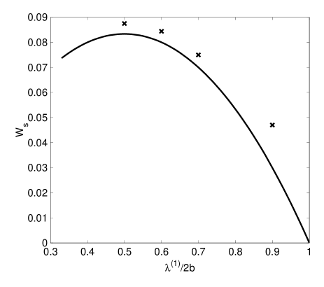
Figure 1: Dependence of the flame velocity increase on the inverse tube width, given by Eq. (86) for the case $\theta=3$, and the results of numerical experiments [5].

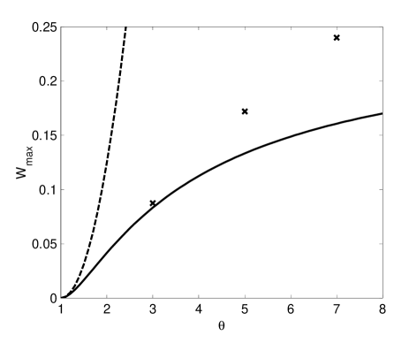
Figure 2: Dependence of the maximal flame velocity increase $W_{{\rm max}}$ on the gas expansion coefficient, given by Eq. (87) (solid line), and calculated on the basis of the Sivashinsky equation (dashed line); the marks are according to the results of [5].

Fig. 1 compares the theoretically predicted dependence of the flame velocity increase on the inverse tube width, given by Eq. (86) for the case $\theta=3$, with the results of numerical experiments [5]. Dependence of the maximal flame velocity increase $W_{{\rm max}}$ on the gas expansion coefficient, given by Eq. (87), is represented in Fig. 2. For comparison, we show also the corresponding dependence calculated with the help of the Sivashinsky equation. We see that the third order equation (78) gives reasonable description of flames with $\theta\sim 3,$ while for larger values of the expansion coefficient it overestimates the influence of vorticity, produced in the flame, on the flame front curvature. In the latter case, therefore, the more accurate fourth order equation (4.1) should be used instead of Eq. (78). Detailed investigation of Eq. (4.1) will be given elsewhere.

5 Large flame velocity expansion

As we have seen, Eq. (3.1) considerably simplifies in the case of small $\alpha.$ For sufficiently narrow tubes, it gives results which turn out to be in a reasonable agreement with the experiment already at the third order in $\alpha.$ Let us now consider the opposite case of very wide tubes, i.e., tubes of width large compared to the cutoff wavelength. As it will be shown presently, under a certain burning regime, Eq. (3.1) can be written in a much simpler form in this case too.

Widely employed in modern jet engines is the process of the so-called fast flow burning (see, e.g., [7], Ch.6, $\S$1). This regime is characterized by a large stretch of the flame front along the tube, since the flame velocity is proportional to the flame front surface (in 2D case, to the front length). Indeed, equating the fuel flow at $\xi=-\infty$ to that through the flame front, using the evolution equation (63), and taking into account the boundary conditions $w=0,$ $f^{\prime}=0,$ one has

$$bV=\int\limits_{0}^{b}dl~{}{\bf n}{\bf v}_{-}=\int\limits_{0}^{b}d\eta(u_{-}-f^{\prime}w_{-})=\int\limits_{0}^{b}d\eta\left\{N-\varepsilon\frac{\theta\ln\theta}{\theta-1}\frac{d}{d\eta}\left(Nw_{-}+f^{\prime}\right)\right\}$$

$$=\int\limits_{0}^{b}d\eta N-\varepsilon\left.\frac{\theta\ln\theta}{\theta-1}\left(Nw_{-}+f^{\prime}\right)\right|_{0}^{b}=l,$$

or

$$V=\frac{l}{b}\gg 1,$$

where $l$ is the length of the flame front, ${\bf n}$ the unit vector normal to the flame front (pointing to the burnt matter), and $b$ is the tube width.

Under these circumstances, it is natural to develop an expansion of Eq. (3.1) in powers of the inverse flame velocity, $1/V.$ This can be done as follows.

Let us note, first of all, that large value of $V$ implies, in general, that the quantity $\upsilon$ (and, therefore, the quantity $\hat{H}\upsilon$ – the $\eta$-component of the fuel velocity at the flame front) is also large. Indeed, as it follows from the evolution equation (11), $\upsilon=1-V$ at the tube wall, in view of the boundary condition $f^{\prime}=0.$ Now, we make the assumption that in the bulk, i.e., for all $\eta$ except for a small region near the points $\eta=0,~{}b,$ the quantity $\upsilon$ is actually of the order $O(1),$ rather than $O(V).$ Then the integral quantity $\hat{H}\upsilon=O(1)+\delta/b~{}O(V)=o(V),$ since the size $\delta$ of the region where $\upsilon\sim V$ is assumed to be small compared with the tube width $b,$ $\delta\ll b$ (see Fig. 3).

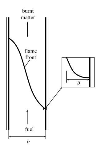
Figure 3: Schematic representation of the flame front shape in the fast flow burning regime.

Expansion of Eq. (3.1) in powers of $1/V$ is straightforward. Below, this expansion will be carried out only to the lowest nontrivial order. As in Sec.4, Eq. (30) for the phase integrates at this order. Therefore, it is more convenient to work with the integral version (47) of the equation (3.1) from the very beginning.

Let us first consider the question concerning the form of the quantities $\Omega,$ $\phi$ entering this equation. As we saw in Sec. 3.1, the value (35) of the constant $C$ in the expression (34) for the amplitude $\Omega$ is fixed up to the second order in $\alpha.$ Furthermore, it was shown in Sec. 3.2, that within the accuracy of our model, the form of Eq. (3.1) is independent of a particular completion of $C$ beyond the order $\alpha^{2},$ and that the value of $C,$ together with values of the arbitrary constants of integration of Eq. (3.1), can be deduced from the boundary conditions. In contrast, the boundary conditions cannot be used directly in the framework of the $1/V$-expansion, since this expansion breaks down near the tube walls. Instead, the value of the constant $C$ as well as the constant $\phi_{0}$ of integration of Eq. (33) will be determined from the requirement of self-consistency of the limiting transition $V\to\infty$ in Eq. (47).

Under assumption $\upsilon,~{}\hat{H}\upsilon\sim o(V),$ it follows from Eq. (36) that $\phi^{\prime}\to 0$ in the bulk when $V\to\infty;$ therefore, $\phi=\phi_{0}={\rm const}.$ On the other hand, the amplitude $\Omega\to\sqrt{\theta V^{2}+C}$ in the same limit. Thus, Eq. (47) gives in the lowest order in $1/V:$

$$\phi_{0}=-\hat{H}\ln\frac{\sqrt{\theta V^{2}+C}}{\theta V}.$$

This equality is only consistent with the properties of the Hilbert operator if

$$\ln\frac{\sqrt{\theta V^{2}+C}}{\theta V}=0,$$

and therefore,

$$\phi_{0}=0,~{}~{}C=\theta(\theta-1)V^{2}.$$ (88)

Note that in the case of small $\alpha,$ the values (88) for the constants $C,$ $\phi_{0}$ coincide with those found in Secs. 3.1, 4.1, respectively, up to the order $\alpha^{2}$. On the other hand, expansion of Eq. (47) in powers of $\upsilon/V$ has the strict validity in this case, since $\upsilon\sim O(\alpha^{2}),$ $V=1+O(\alpha^{2})$ for all $\eta\in(0,~{}b).$ We conclude, therefore, that the first order of the large $V$ expansion of Eq. (47) must automatically reproduce the second order of the small $\alpha$ expansion of this equation, i.e., the Sivashinsky equation (76).

Substituting Eq. (88) into Eq. (47) and expanding to the first order in $\upsilon/V$ gives

$$\frac{V\left(\hat{H}\upsilon-f^{\prime}\frac{\theta-1}{N}\right)}{\theta^{2}V^{2}}=-\hat{H}\frac{\upsilon}{\theta V},$$

or

$$\upsilon=-\frac{\theta-1}{\theta+1}\hat{H}\left(\frac{f^{\prime}}{N}\right).$$ (89)

Since the flame is highly stretched in the fast flow burning regime, the slope $f^{\prime}$ of the flame front is large. However, it follows from Eq. (89) that the quantities $\upsilon$ and $\hat{H}\upsilon$ remain of the order O(1), since $f^{\prime}/N<1.$ Our initial assumption is thus confirmed.

Substituting Eq. (89) into the evolution equation (25), we obtain

$$N-V=-\frac{\theta-1}{\theta+1}(f^{\prime}+\hat{H})\left(\frac{f^{\prime}}{N}\right).$$ (90)

We see that in the case of small $\theta-1,$ Eq. (90) does reproduce the stationary part of the Sivashinsky equation (76) in the case $\varepsilon=0.$

Finally, it is not difficult to take into account the influence of the small flame thickness. First of all, we note from Eq. (89) that although the quantity $\upsilon=O(1),$ its $\eta$-derivative

$$\upsilon^{\prime}=-\frac{\theta-1}{\theta+1}\hat{H}\left(\frac{f^{\prime}}{N}\right)^{\prime}=-\frac{\theta-1}{\theta+1}\hat{H}\left(\frac{f^{\prime\prime}}{N^{3}}\right)=O\left(\frac{1}{V^{2}}\right),$$

since $f^{\prime\prime},N\sim f^{\prime}\sim V.$ It follows then from Eqs. (64)–(66) that $\hat{D}u_{-},~{}\hat{D}w_{-}=O(1/V).$ Resolving Eqs. (60), (61) with respect to $u_{+},~{}w_{+},$ we see that the $\varepsilon$-corrections to these quantities are only of the relative order $1/V^{2}.$ Analogously, the $\varepsilon$-correction in the pressure jump (3.3) is $O(1),$ which implies the same $O(1/V^{2})$ relative correction in the amplitude $\Omega.$ Thus, we conclude that Eq. (47) remains unchanged in the first order in $1/V,$ and so does, therefore, its consequence, Eq. (89). Substituting the latter into evolution equation (63), we obtain

$$N-V=-\frac{\theta-1}{\theta+1}(f^{\prime}+\hat{H})\left(\frac{f^{\prime}}{N}\right)+\varepsilon\frac{2\theta^{2}\ln\theta}{\theta^{2}-1}f^{\prime\prime}.$$ (91)

It is interesting to note that the term describing the influence of finite flame thickness turns out to be linear in $f.$

6 Discussion and conclusions

We have shown that in the stationary case, the asymptotic expansion of the nonlinear equation for the flame front position can be pushed beyond the second order in $\theta-1,$ at which the gas flow is potential on both sides of the flame front, to take into account vorticity drift behind the flame front. This expansion has been carried out explicitly; for the case of ideal tube walls, it is given by Eqs. (78), (4.1) at the third and fourth orders, respectively. Remarkably, the third order equation, which describes influence of the vorticity on the flame front structure to the lowest nontrivial order, turns out to have the same functional structure as the Sivashinsky equation. As we showed in Sec. 4.2, it gives results in a reasonable agreement with the numerical experiments on the flame propagation in tubes for the case of flames with $\theta\leq 3.$

It should be mentioned that the nonlinear equation for the flame front, derived in Ref. [10], also gives satisfactory description of the stationary flame propagation in narrow tubes. We showed already in the Introduction that the approach of Ref. [10] is self-contradictory. Still, one might imagine that despite an erroneous derivation, the resulting equation is correct. However, the results of Sec. 4.1 show that in the case $\theta\to 1,$ asymptotic expansion of the true nonlinear equation is quite different from that of the equation proposed in Ref. [10]. The latter is incorrect, therefore, already in the case of small gas expansion.

From a more general point of view, the theory of flame propagation in the fully developed nonlinear regime cannot be formulated in the way the Sivashinsky equation [8] or the Frankel equation [9] are formulated. This is because the assumption of potentiality of the flow downstream, employed in these works, renders the relations between the flow variables local, allowing thereby the formulation of equation for the flame front position in terms of this position alone. In contrast, account of the vorticity production in the flame makes the problem essentially nonlocal, since, e.g., the value of the pressure field on the flame front is a functional of the velocity field in the bulk, which implies, in particular, that the equation for the flame front position must be a functional of the boundary conditions. Indeed, as we saw in Sec. 4.1, the boundary conditions on the tube walls are invoked in the course of derivation of the asymptotic expansion of this equation already at the third order.

Finally, with the help of the general equation (3.1), highly nonlinear regimes of the stationary flame propagation can be considered. We would like to remind that this equation respects all the conservation laws to be satisfied across the flame front, by construction. Thus, despite the fact that the vorticity drift behind the flame front is taken into account in this equation on the basis of the model assumption (15), unjustified for arbitrary $\theta,$ one may hope that it gives at least qualitative description. We showed in Sec. 5 that in the particular case of the fast flow burning, equation (3.1) (as well as its generalization to the case of nonzero flame thickness) can be highly simplified by expanding it in powers of the inverse flame velocity. The result of this expansion to the first order is given by Eq. (91).

Acknowledgements

We are grateful to V. V. Bychkov for interesting discussions.

This research was supported in part by Swedish Ministry of Industry (Energimyndigheten, contract P 12503-1), by the Swedish Research Council (contract E5106-1494/2001), and by the Swedish Royal Academy of Sciences.

7 Appendix

For the sake of completeness, we give here a brief account of the properties of the Hilbert operator, used in the text.

Given a sufficiently smooth integrable function $f(\eta),$ $\eta\in(-\infty,+\infty),$ the Hilbert operator $\hat{H}$ is defined by

$$(\hat{H}f)(\eta)=\frac{1}{\pi}{\rm p.v.}\int\limits_{-\infty}^{+\infty}d\zeta\frac{f(\zeta)}{\zeta-\eta},$$ (92)

$"{\rm p.v.}"$ denoting the principal value. By definition, operator $\hat{H}$ is linear, i.e., for any complex numbers $c_{1},$ $c_{2},$

$$\hat{H}(c_{1}f_{1}+c_{2}f_{2})=c_{1}\hat{H}f_{1}+c_{2}\hat{H}f_{2},$$

and real, i.e.,

$$(\hat{H}f)^{*}=\hat{H}f^{*},$$

where $F^{*}$ denotes the complex conjugate of $F.$

It is convenient to introduce the usual scalar product of two functions $f_{1}(\eta)$ and $f_{2}(\eta)$

$$(f_{1},f_{2})=\int\limits_{-\infty}^{+\infty}d\eta f_{1}^{*}(\eta)f_{2}(\eta).$$

Then, changing the order of integration, one has

$$(f_{1},\hat{H}f_{2})=\frac{1}{\pi}\int\limits_{-\infty}^{+\infty}d\eta f_{1}^{*}(\eta){\rm p.v.}\int\limits_{-\infty}^{+\infty}d\zeta\frac{f_{2}(\zeta)}{\zeta-\eta}=-\frac{1}{\pi}\int\limits_{-\infty}^{+\infty}d\zeta f_{2}(\zeta){\rm p.v.}\int\limits_{-\infty}^{+\infty}d\eta\frac{f_{1}^{*}(\eta)}{\eta-\zeta}=-(\hat{H}f_{1},f_{2}),$$

or

$$(f_{1},\hat{H}f_{2})=-(\hat{H}f_{1},f_{2}),$$ (93)

i.e., the Hilbert operator is anti-Hermitian.

To prove the operator identity

$$\hat{H}^{2}=-1,$$ (94)

it is convenient to represent the right hand side of Eq. (92) as the integral over the contour $C_{1}=C_{1}^{-}\cup C_{1}^{+}$ in the complex $\eta$-plane (see Fig. 4)

$$(\hat{H}f)(\eta)=\frac{1}{2\pi}\int\limits_{C_{1}}dz\frac{f(z)}{z-\eta}.$$ (95)

Then the square of the Hilbert operator takes the form

$$(\hat{H}^{2}f)(\eta)=\frac{1}{4\pi^{2}}\int\limits_{C_{1}}\frac{d\tilde{z}}{\tilde{z}-\eta}\int\limits_{C_{2}}dz\frac{f(z)}{z-\tilde{z}},$$ (96)

where the contour $C_{2}=C_{2}^{-}\cup C_{2}^{+}$ comprises $C_{1}.$ Changing the order of integration in Eq. (96), using the formula

$$\int\frac{d\tilde{z}}{(\tilde{z}-\eta)(z-\tilde{z})}=\frac{1}{z-\eta}\ln\frac{\tilde{z}-\eta}{\tilde{z}-z},$$

and taking into account that the logarithm gives rise to a nonzero contribution only if the arguments of the functions $\tilde{z}-\eta$ and $\tilde{z}-z$ run in opposite directions when $\tilde{z}$ runs the contours $C_{1}^{\pm},$ we obtain

$$\frac{1}{4\pi^{2}}\int\limits_{C_{1}}\frac{d\tilde{z}}{\tilde{z}-\eta}\int\limits_{C_{2}}dz\frac{f(z)}{z-\tilde{z}}=\frac{1}{4\pi^{2}}\left(2\pi i\int\limits_{C_{2}^{-}}dz\frac{f(z)}{z-\eta}-2\pi i\int\limits_{C_{2}^{+}}dz\frac{f(z)}{z-\eta}\right)$$

$$=\frac{i}{2\pi}\int\limits_{C}dz\frac{f(z)}{z-\eta},$$

and therefore,

$$(\hat{H}^{2}f)(\eta)=-f(\eta).$$

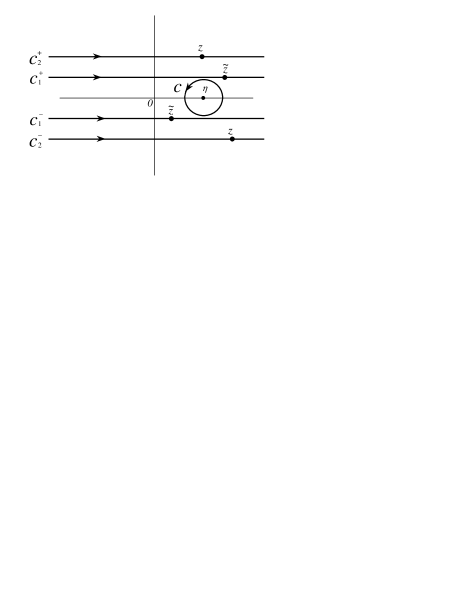
Figure 4: Contours of integration in Eqs. (95)–(7).

Next, let us consider the quantity

$$(\hat{H}\{f\hat{H}f\})(\eta)=\frac{1}{4\pi^{2}}\int\limits_{C_{1}}d\tilde{z}\frac{f(\tilde{z})}{\tilde{z}-\eta}\int\limits_{C_{2}}dz\frac{f(z)}{z-\tilde{z}}$$

$$=\frac{1}{4\pi^{2}}\int\limits_{C_{1}}d\tilde{z}\frac{f(\tilde{z})}{\tilde{z}-\eta}\int\limits_{C_{2}}dz\frac{f(z)}{z-\eta}-\frac{1}{4\pi^{2}}\int\limits_{C_{2}}dz\frac{f(z)}{z-\eta}\int\limits_{C_{1}}d\tilde{z}\frac{f(\tilde{z})}{\tilde{z}-z}.$$ (97)

The first term in the right hand side of Eq. (7) is just $\{(\hat{H}f)(\eta)\}^{2}.$ The second term can be transformed as follows. The contour $C_{1}^{-}$ of the $\tilde{z}$-integral can be moved down pass the contour $C_{2}^{-},$ the pole at $\tilde{z}=z$ giving rise to the extra term $-2\pi if(z),$ $z\in C_{2}^{-}.$ Likewise, $C_{1}^{+}$ can be moved up pass $C_{2}^{+},$ with the extra term $2\pi if(z),$ $z\in C_{2}^{+}.$ Thus,

$$\frac{1}{4\pi^{2}}\int\limits_{C_{2}}dz\frac{f(z)}{z-\eta}\int\limits_{C_{1}}d\tilde{z}\frac{f(\tilde{z})}{\tilde{z}-z}=\frac{1}{4\pi^{2}}\int\limits_{C_{1}}dz\frac{f(z)}{z-\eta}\int\limits_{C_{2}}d\tilde{z}\frac{f(\tilde{z})}{\tilde{z}-z}$$

$$-\frac{i}{2\pi}\left(\int\limits_{C_{2}^{-}}dz\frac{f^{2}(z)}{z-\eta}-\int\limits_{C_{2}^{+}}dz\frac{f^{2}(z)}{z-\eta}\right)=\frac{1}{4\pi^{2}}\int\limits_{C_{1}}d\tilde{z}\frac{f(\tilde{z})}{\tilde{z}-\eta}\int\limits_{C_{2}}dz\frac{f(z)}{z-\tilde{z}}$$

$$-\frac{i}{2\pi}\int_{C}dz\frac{f^{2}(z)}{z-\eta}=(\hat{H}\{f\hat{H}f\})(\eta)+f^{2}(\eta).$$

Substituting this into Eq. (7), we arrive at the following identity

$$2\hat{H}\{f\hat{H}f\}=(\hat{H}f)^{2}-f^{2}.$$ (98)

Finally, let us establish the connection

$$\hat{\Phi}=-\partial\hat{H}$$ (99)

between the 2D Landau-Darrieus operator $\hat{\Phi}$ and the Hilbert operator. The former is defined by

$$(\hat{\Phi}f)(\eta)=\int\limits_{-\infty}^{+\infty}dk|k|f_{k}e^{ik\eta},$$

$f_{k}$ being the Fourier transform of $f.$ Using the Fourier representation of the function $"{\rm sign}"$

$${\rm sign}(k)=\frac{1}{2\pi i}\int\limits_{-\infty}^{+\infty}e^{ik\zeta}\left(\frac{1}{\zeta-i0}+\frac{1}{\zeta+i0}\right),$$

one has

$$(\hat{\Phi}f)(\eta)=\int\limits_{-\infty}^{+\infty}dk~{}k~{}{\rm sign}(k)f_{k}e^{ik\eta}$$

$$=-\frac{1}{2\pi}\frac{\partial}{\partial\eta}\int\limits_{-\infty}^{+\infty}d\zeta\left(\frac{1}{\zeta-i0}+\frac{1}{\zeta+i0}\right)\int\limits_{-\infty}^{+\infty}dk~{}f_{k}e^{ik(\eta+\zeta)}$$

$$=-\frac{1}{2\pi}\frac{\partial}{\partial\eta}\int\limits_{-\infty}^{+\infty}d\zeta f(\eta+\zeta)\left(\frac{1}{\zeta-i0}+\frac{1}{\zeta+i0}\right)=-\frac{1}{\pi}\frac{\partial}{\partial\eta}{\rm p.v.}\int\limits_{-\infty}^{+\infty}d\zeta\frac{f(\eta+\zeta)}{\zeta},$$

or

$$(\hat{\Phi}f)(\eta)=-\frac{\partial}{\partial\eta}(\hat{H}f)(\eta).$$

Eq. (99) is convenient in estimating the orders of magnitude of expressions involving the operator $\hat{\Phi}.$ In view of Eqs. (93) and (94), one has

$$(\hat{H}f,\hat{H}f)=-(\hat{H}^{2}f,f)=(f,f),$$

i.e., the Hilbert operator has unit norm, and therefore

$$\hat{\Phi}f=O(\partial f).$$

References

- [1] L. D. Landau, ”On the theory of slow combustion”, Acta Physicochimica URSS 19, 77 (1944).
- [2] G. Darrieus, Propagation d’un front de flamme, Presented at Le congres de Mecanique Appliquee (1945)(unpublished).
- [3] P. Pelce and P. Clavin, ”Influences of hydrodynamics and diffusion upon the stability limits of laminar premixed flames”, J. Fluid Mech. 124, 219 (1982).
- [4] D. M. Michelson and G. I. Sivashinsky, ”Nonlinear analysis of hydrodynamic instability in laminar flames”, Acta Astronaut. 4, 1207 (1977).
- [5] V. V. Bychkov, S. M. Golberg, M. A. Liberman, and L. E. Eriksson, ”Propagation of curved stationary flames in tubes”, Phys. Rev. E54, 3713 (1996).
- [6] Ya. B. Zel’dovich, ”An effect stabilizing curved laminar flame front”, Prikl.Mat.Teor.Fiz. 1, 102 (1966) (in russian).
- [7] Ya. B. Zel’dovich, G. I. Barenblatt, V. B. Librovich, and G. M. Makhviladze, The Mathematical Theory of Combustion and Explosion (Consultants Bureau, New York, 1985).
- [8] G. I. Sivashinsky, ”Nonlinear analysis of hydrodinamic instability in laminar flames”, Acta Astronaut. 4, 1177 (1977).
- [9] M. L. Frankel, ”An equation of surface dynamics modelling flame fronts as density discontinuies in potential flow”, Phys. Fluids A 2, 1879 (1990).
- [10] V. V. Bychkov, ”Nonlinear equation for a curved stationary flame and the flame velocity”, Phys. Fluids. 10, 2091 (1998).
- [11] V. V. Bychkov, K. A. Kovalev, and M. A. Liberman, Phys. Rev. E60, 2897 (1999).
- [12] M. Matalon and B. J. Matkowsky, ”Flames as gasdynamic discontinuities”, J. Fluid Mech. 124, 239 (1982).
- [13] S. K. Zhdanov and B. A. Trubnikov, J. Exp. Theor. Phys. 68, 65 (1989).
- [14] L.D. Landau, E.M. Lifshitz, Fluid Mechanics (Pergamon, Oxford, 1987).
- [15] O. Thual, U. Frish, and M. Henon, ”Application of pole decomposition to an equation governing the dynamics of wrinkled flames”, J. Phys. (France) 46, 1485 (1985).
- [16] G. Joulin, ”On the Zhdanov-Trubnikov equation for premixed flame stability”, J. Exp. Theor. Phys. 73, 234 (1991).
- [17] M. Rahibe, N. Aubry, G. I. Sivashinsky, and R. Lima, ”Formation of wrinkles in outwardly propagating flames”, Phys. Rev. E52, 3675 (1995).
- [18] M. Rahibe, N. Aubry, and G. I. Sivashinsky, ”Stability of pole solutions for planar propagating flames”, Phys. Rev. E54, 4958 (1996).
- [19] M. Rahibe, N. Aubry, and G. I. Sivashinsky, ”Instability of pole solutions for planar propagating flames in sufficiently large domains”, Combust. Theory Modelling 2, 19 (1998).