Resonant-state solution of the Faddeev-Merkuriev integral equations for three-body systems with Coulomb potentials

Abstract

A novel method for calculating resonances in three-body Coulombic systems is proposed. The Faddeev-Merkuriev integral equations are solved by applying the Coulomb-Sturmian separable expansion method. The $e^{-}e^{+}e^{-}$ S-state resonances up to $n=5$ threshold are calculated.

]

I Introduction

For three-body systems the Faddeev equations are the fundamental equations. Three-body bound states correspond to the solutions of the homogeneous Faddeev equations at real energies, and resonances, as is usual in quantum mechanics, are related to complex-energy solutions.

The Faddeev equations were derived for short-range interactions. However, if we simply plug-in a Coulomb-like potential they become singular. A formally exact approach was proposed by Noble [1]. His formulation was designed for solving the nuclear three-body Coulomb problem, where all Coulomb interactions were repulsive. The interactions were split into short-range and long-range Coulomb-like parts and the long-range parts were formally included in the ”free” Green’s operator. Merkuriev extended the idea of Noble by performing the splitting in the three-body configuration space [2]. This was a crucial development since it made possible to treat attractive Coulomb interactions on an equal footing with repulsive ones.

Recently we have presented a method for treating the three-body Coulomb scattering problem by solving Faddeev-Merkuriev integral equations using the Coulomb-Sturmian separable expansion technique [3]. We solved the inhomogeneous Faddeev-Merkuriev integral equations for real energies. Previously, for calculating resonances in three-body systems with short-range plus repulsive Coulomb interactions, we solved homogeneous Faddeev-Noble integral equations by using the Coulomb-Sturmian separable expansion technique [4]. In this paper by combining the concepts of Refs.  [3] and [4] we solve the homogeneous Faddeev-Merkuriev integral equations for complex energies. This way we can handle all kind of Coulomb-like potentials in resonant-state calculations, not only repulsive but also attractive ones.

In section II we present the homogeneous Faddeev-Merkuriev integral equations, outlined for systems where two particles out of the three are identical. Many systems, like $e^{-}e^{+}e^{-}$ and $H^{-}$, fall into this category. Then, in section III, we present the solution method adapted to the case where all charges have the same absolute value. In section IV we present our calculations for the $L=0$ resonances of the $e^{-}e^{+}e^{-}$ system up to the $n=5$ threshold and compare them with the results of complex scaling calculations [5].

II Faddeev-Merkuriev integral equations

The Hamiltonian of a three-body Coulombic system reads

$$H=H^{0}+v_{1}^{C}+v_{2}^{C}+v_{3}^{C},$$ (1)

where $H^{0}$ is the three-body kinetic energy operator and $v_{\alpha}^{C}$ denotes the Coulomb-like interaction in the subsystem $\alpha$. We use throughout the usual configuration-space Jacobi coordinates $x_{\alpha}$ and $y_{\alpha}$. Thus $v_{\alpha}^{C}$ only depends on $x_{\alpha}$ ($v_{\alpha}^{C}=v_{\alpha}^{C}(x_{\alpha})$). The Hamiltonian (1) is defined in the three-body Hilbert space. The two-body potential operators are formally embedded in the three-body Hilbert space

$$v^{C}=v^{C}(x){\bf 1}_{y},$$ (2)

where ${\bf 1}_{y}$ is a unit operator in the two-body Hilbert space associated with the $y$ coordinate. We also use the notation $X=\{x_{\alpha},y_{\alpha}\}\in{\bf R}^{6}$.

The role of Coulomb potentials in Hamiltonian (1) are twofold. Their long-distance parts modify the asymptotic motion, while their short-range parts strongly correlate the two-body subsystems. Merkuriev introduced a separation of the three-body configuration space into different asymptotic regions. The two-body asymptotic region $\Omega_{\alpha}$ is defined as a part of the three-body configuration space where the conditions

$$|x_{\alpha}|<x^{0}_{\alpha}(1+|y_{\alpha}|/y^{0}_{\alpha})^{1/\nu},$$ (3)

with $x^{0}_{\alpha},y^{0}_{\alpha}>0$ and $\nu>2$, are satisfied. Merkuriev proposed to split the Coulomb interaction in the three-body configuration space into short-range and long-range terms

$$v_{\alpha}^{C}=v_{\alpha}^{(s)}+v_{\alpha}^{(l)},$$ (4)

where the superscripts $s$ and $l$ indicates the short- and long-range attributes, respectively. The splitting is carried out with the help of a splitting function $\zeta_{\alpha}$ which possesses the property

$$\zeta_{\alpha}(x_{\alpha},y_{\alpha})\xrightarrow{X_{\alpha}\to\infty}\left\{\begin{array}[]{ll}1,&X_{\alpha}\in\Omega_{\alpha}\\ 0&\mbox{otherwise.}\end{array}\right.$$ (5)

In practice, in the configuration-space differential equation approaches, usually the functional form

$$\zeta(x,y)=2/\left\{1+\exp\left[{(x/x^{0})^{\nu}}/{(1+y/y^{0})}\right]\right\},$$ (6)

was used.

The long-range Hamiltonian is defined as

$$H^{(l)}=H^{0}+v_{1}^{(l)}+v_{2}^{(l)}+v_{3}^{(l)},$$ (7)

and its resolvent operator is

$$G^{(l)}(z)=(z-H^{(l)})^{-1},$$ (8)

where $z$ is the complex energy-parameter. Then, the three-body Hamiltonian takes the form

$$H=H^{(l)}+v_{1}^{(s)}+v_{2}^{(s)}+v_{3}^{(s)},$$ (9)

which formally looks like a three-body Hamiltonian with short-range potentials. Therefore the Faddeev method is applicable.

In the Faddeev procedure we split the wave function into three components

$$|\Psi\rangle=|\psi_{1}\rangle+|\psi_{2}\rangle+|\psi_{3}\rangle,$$ (10)

where the components are defined by

$$|\psi_{\alpha}\rangle=G^{(l)}(z)v_{\alpha}^{(s)}|\Psi\rangle.$$ (11)

In case of bound and resonant states the wave-function components satisfy the homogeneous Faddeev-Merkuriev integral equations

$$|\psi_{1}\rangle = G_{1}^{(l)}(z)v^{(s)}_{1}[|\psi_{2}\rangle+|\psi_{3}\rangle]$$ (12)

$$|\psi_{2}\rangle = G_{2}^{(l)}(z)v^{(s)}_{2}[|\psi_{1}\rangle+|\psi_{3}\rangle]$$ (13)

$$|\psi_{3}\rangle = G_{3}^{(l)}(z)v^{(s)}_{3}[|\psi_{1}\rangle+|\psi_{2}\rangle]$$ (14)

at real and complex energies, respectively. Here $G^{(l)}_{\alpha}$ is the resolvent of the channel long-ranged Hamiltonian

$$H^{(l)}_{\alpha}=H^{(l)}+v_{\alpha}^{(s)},$$ (15)

$G^{(l)}_{\alpha}(z)=(z-H^{(l)}_{\alpha})^{-1}$. Merkuriev has proved that Eqs. (12-14) possess compact kernels, and this property remains valid also for complex energies $z=E-i\Gamma/2$, $\Gamma>0$.

In atomic three-particle systems the sign of the charge of two particles are always identical. Let us denote them by $1$ and $2$, and the non-identical one by $3$. In this case $v_{3}^{C}$ is a repulsive Coulomb potential which does not support two-body bound states. Therefore the entire $v_{3}^{C}$ can be considered as long-range potential. The long-range Hamiltonian is modified as

$$H^{(l)}=H^{0}+v_{1}^{(l)}+v_{2}^{(l)}+v_{3}^{C}.$$ (16)

Then, the three-body Hamiltonian takes the form

$$H=H^{(l)}+v_{1}^{(s)}+v_{2}^{(s)},$$ (17)

i.e. the Hamiltonian of the system appears formally as a three-body Hamiltonian with two short-range potentials. Therefore the Faddeev procedure, in this case, gives a set of two-component Faddeev-Merkuriev integral equations

$$|\psi_{1}\rangle = G_{1}^{(l)}v_{1}^{(s)}|\psi_{2}\rangle$$ (18)

$$|\psi_{2}\rangle = G_{2}^{(l)}v_{2}^{(s)}|\psi_{1}\rangle.$$ (19)

Further simplification can be achieved if the particles $1$ and $2$ are identical. Then, the Faddeev components $|\psi_{1}\rangle$ and $|\psi_{2}\rangle$, in their own natural Jacobi coordinates, have the same functional form

$$\langle x_{1}y_{1}|\psi_{1}\rangle=\langle x_{2}y_{2}|\psi_{2}\rangle=\langle xy|\psi\rangle.$$ (20)

Therefore we can determine $|\psi\rangle$ from the first equation only

$$|\psi\rangle=G_{1}^{(l)}v_{1}^{(s)}p{\mathcal{P}}|\psi\rangle,$$ (21)

where ${\mathcal{P}}$ is the operator for the permutation of indexes $1$ and $2$ and $p=\pm 1$ are eigenvalues of ${\mathcal{P}}$. We note that although this integral equation has only one component yet gives full account on asymptotic and symmetry properties of the system.

III Solution method

We solve these integral equations by using the Coulomb–Sturmian separable expansion approach [6]. The Coulomb-Sturmian (CS) functions are defined by

$$\langle r|nl\rangle=\left[\frac{n!}{(n+2l+1)!}\right]^{1/2}(2br)^{l+1}\exp(-br)L_{n}^{2l+1}(2br),$$ (22)

with $n$ and $l$ being the radial and orbital angular momentum quantum numbers, respectively, and $b$ is the size parameter of the basis. The CS functions $\{|nl\rangle\}$ form a biorthonormal discrete basis in the radial two-body Hilbert space; the biorthogonal partner defined by $\langle r|\widetilde{nl}\rangle=\langle r|{nl}\rangle/r$. Since the three-body Hilbert space is a direct product of two-body Hilbert spaces an appropriate basis can be defined as the angular momentum coupled direct product of the two-body bases

$$|n\nu l\lambda\rangle_{\alpha}=|nl\rangle_{\alpha}\otimes|\nu\lambda\rangle_{\alpha},\ \ \ \ (n,\nu=0,1,2,\ldots),$$ (23)

where $|nl\rangle_{\alpha}$ and $|\nu\lambda\rangle_{\alpha}$ are associated with the coordinates $x_{\alpha}$ and $y_{\alpha}$, respectively. With this basis the completeness relation takes the form (with angular momentum summation implicitly included)

$${\bf 1}=\lim\limits_{N\to\infty}\sum_{n,\nu=0}^{N}|\widetilde{n\nu l\lambda}\rangle_{\alpha}\;\mbox{}_{\alpha}\langle{n\nu l\lambda}|=\lim\limits_{N\to\infty}{\bf 1}^{N}_{\alpha}.$$ (24)

Note that in the three-body Hilbert space, three equivalent bases belonging to fragmentation $1$, $2$ and $3$ are possible.

We make the following approximation on the set of Faddeev-Merkuriev integral equations

$$|\psi_{1}\rangle = G_{1}^{(l)}(z){\bf 1}^{N}_{1}v^{(s)}_{1}[{\bf 1}^{N}_{2}|\psi_{2}\rangle+{\bf 1}^{N}_{3}|\psi_{3}\rangle]$$ (25)

$$|\psi_{2}\rangle = G_{2}^{(l)}(z){\bf 1}^{N}_{2}v^{(s)}_{2}[{\bf 1}^{N}_{1}|\psi_{1}\rangle+{\bf 1}^{N}_{3}|\psi_{3}\rangle]$$ (26)

$$|\psi_{3}\rangle = G_{3}^{(l)}(z){\bf 1}^{N}_{3}v^{(s)}_{3}[{\bf 1}^{N}_{1}|\psi_{1}\rangle+{\bf 1}^{N}_{2}|\psi_{2}\rangle],$$ (27)

i.e. the short-range potential $v_{\alpha}^{(s)}$ in the three-body Hilbert space is taken to have a separable form, viz.

$$v_{\alpha}^{(s)} = \lim_{N\to\infty}{\bf 1}^{N}_{\alpha}v_{\alpha}^{(s)}{\bf 1}^{N}_{\beta}$$ (28)

$$\approx {\bf 1}^{N}_{\alpha}v_{\alpha}^{(s)}{\bf 1}^{N}_{\beta}=\sum_{n,\nu,n^{\prime},\nu^{\prime}=0}^{N}|\widetilde{n\nu l\lambda}\rangle_{\alpha}\;\underline{v}_{\alpha\beta}^{(s)}\;\mbox{}_{\beta}\langle\widetilde{n^{\prime}\nu^{\prime}l^{\prime}\lambda^{\prime}}|,$$ (29)

where $\underline{v}_{\alpha\beta}^{(s)}=\mbox{}_{\alpha}\langle n\nu l\lambda|v_{\alpha}^{(s)}|n^{\prime}\nu^{\prime}l^{\prime}\lambda^{\prime}\rangle_{\beta}$. In Eq. (29) the ket and bra states are defined for different fragmentation, depending on the environment of the potential operators in the equations. The validity of this approximation relies on the square integrable property of the terms like $v_{\alpha}^{(s)}|\psi_{\beta}\rangle$, which is guaranteed due to the short range nature of $v_{\alpha}^{(s)}$.

For solving Eq. (21) we proceed in a similar way,

$$|\psi\rangle=G_{1}^{(l)}{\bf 1}^{N}_{1}v_{1}^{(s)}p{\mathcal{P}}{\bf 1}^{N}_{1}|\psi\rangle,$$ (30)

i.e. the operator $v_{1}^{(s)}p{\mathcal{P}}$ in the three-body Hilbert space is approximated by a separable form, viz.

$$v_{1}^{(s)}p{\mathcal{P}} = \lim_{N\to\infty}{\bf 1}^{N}_{1}v_{1}^{(s)}p{\mathcal{P}}{\bf 1}^{N}_{1}$$ (31)

$$\approx {\bf 1}^{N}_{1}v_{1}^{(s)}p{\mathcal{P}}{\bf 1}^{N}_{1}$$ (32)

$$\approx \sum_{n,\nu,n^{\prime},\nu^{\prime}=0}^{N}|\widetilde{n\nu l\lambda}\rangle_{1}\;\underline{v}_{1}^{(s)}\;\mbox{}_{1}\langle\widetilde{n^{\prime}\nu^{\prime}l^{\prime}\lambda^{\prime}}|,$$ (33)

where $\underline{v}_{1}^{(s)}=\mbox{}_{1}\langle n\nu l\lambda|v_{1}^{(s)}p{\mathcal{P}}|n^{\prime}\nu^{\prime}l^{\prime}\lambda^{\prime}\rangle_{1}$. Utilizing the properties of the exchange operator ${\mathcal{P}}$ these matrix elements can be written in the form $\underline{v}_{1}^{(s)}=p\times\mbox{}_{1}\langle n\nu l\lambda|v_{1}^{(s)}|n^{\prime}\nu^{\prime}l^{\prime}\lambda^{\prime}\rangle_{2}$.

With this approximation, the solution of Eq. (21) turns into solution of matrix equations for the component vector $\underline{\psi}_{1}=\mbox{}_{1}\langle\widetilde{n\nu l\lambda}|\psi_{1}\rangle$

$$\{[\underline{G}^{(l)}_{1}(z)]^{-1}-\underline{v}^{(s)}_{1}\}\underline{\psi}_{1}=0,$$ (34)

where $\underline{G}_{1}^{(l)}=\mbox{}_{1}\langle\widetilde{n\nu l\lambda}|G_{1}^{(l)}|\widetilde{n^{\prime}\nu^{\prime}l^{\prime}\lambda^{\prime}}\rangle_{1}$. A unique solution exists if and only if

$$\det\{[\underline{G}^{(l)}_{1}(z)]^{-1}-\underline{v}^{(s)}_{1}\}=0.$$ (35)

Unfortunately $\underline{G}_{1}^{(l)}$ is not known. It is related to the Hamiltonian $H_{1}^{(l)}$, which itself is a complicated three-body Coulomb Hamiltonian. In the three-potential formalism [3] $\underline{G}_{1}^{(l)}$ is linked to simpler quantities via solution of a Lippmann-Schwinger equation,

$$(\underline{G}^{(l)}_{1})^{-1}=(\underline{\widetilde{G}}_{1})^{-1}-\underline{U}_{1},$$ (36)

where

$${\underline{\widetilde{G}}_{1}}_{n\nu l\lambda,n^{\prime}\nu^{\prime}l^{\prime}{\lambda}^{\prime}}=\mbox{}_{1}\langle\widetilde{n\nu l\lambda}|\widetilde{G}_{1}|\widetilde{n^{\prime}\nu^{\prime}l^{\prime}{\lambda}^{\prime}}\rangle_{1}$$ (37)

and

$${\underline{U}_{1}}_{n\nu l\lambda,n^{\prime}\nu^{\prime}l^{\prime}{\lambda}^{\prime}}=\mbox{}_{1}\langle n\nu l\lambda|U_{1}|n^{\prime}\nu^{\prime}l^{\prime}{\lambda}^{\prime}\rangle_{1}.$$ (38)

In our special case, where the sum of the charges of particles $2$ and $3$ is zero, the operator $\widetilde{G}_{1}$ is the resolvent operator of the Hamiltonian

$$\widetilde{H}_{1}=H^{0}+v_{1}^{C},$$ (39)

and the polarization potential $U_{1}$ is given by

$$U_{1}=v_{2}^{(l)}+v_{3}^{C}.$$ (40)

The most crucial point in this procedure is the calculation of the matrix elements $\underline{\widetilde{G}}_{1}$, since the potential matrix elements $\underline{v}^{(s)}_{1}$ and $\underline{U}_{1}$ can always be evaluated numerically by making use of the transformation of Jacobi coordinates [7]. The Green’s operator $\widetilde{G}_{\alpha}$ is a resolvent of the sum of two commuting Hamiltonians, $\widetilde{H}_{1}=h_{x_{1}}+h_{y_{1}}$, where $h_{x_{1}}=h^{0}_{x_{1}}+v_{1}^{C}(x_{1})$ and $h_{y_{1}}=h^{0}_{y_{1}}$, which act in different two-body Hilbert spaces. Thus, according to the convolution theorem the three-body Green’s operator $\widetilde{G}_{\alpha}$ equates to a convolution integral of two-body Green’s operators, i.e.

$$\widetilde{G}_{1}(z)=\frac{1}{2\pi{i}}\oint_{C}dz^{\prime}\,g_{x_{1}}(z-z^{\prime})\;g_{y_{1}}(z^{\prime}),$$ (41)

where $g_{x_{1}}(z)=(z-h_{x_{1}})^{-1}$ and $g_{y_{1}}(z)=(z-h_{y_{1}})^{-1}$. The contour $C$ should be taken counterclockwise around the continuous spectrum of $h_{y_{1}}$ such a way that $g_{x_{1}}$ is analytic on the domain encircled by $C$.

To examine the structure of the integrand let us shift the spectrum of $g_{x_{1}}$ by taking $z=E+{i}\varepsilon$ with positive $\varepsilon$. By doing so, the two spectra become well separated and the spectrum of $g_{y_{1}}$ can be encircled. Next the contour $C$ is deformed analytically in such a way that the upper part descends to the unphysical Riemann sheet of $g_{y_{1}}$, while the lower part of $C$ can be detoured away from the cut [see Fig. 3]. The contour still encircles the branch cut singularity of $g_{y_{1}}$, but in the $\varepsilon\to 0$ limit it now avoids the singularities of $g_{x_{1}}$. Moreover, by continuing to negative values of $\varepsilon$, in order that we can calculate resonances, the branch cut and pole singularities of $g_{x_{1}}$ move onto the second Riemann sheet of $g_{y_{1}}$ and, at the same time, the branch cut of $g_{y_{1}}$ moves onto the second Riemann sheet of $g_{x_{1}}$. Thus, the mathematical conditions for the contour integral representation of $\widetilde{G}_{1}(z)$ in Eq. (41) can be fulfilled also for complex energies with negative imaginary part. In this respect there is only a gradual difference between the bound- and resonant-state calculations. Now, the matrix elements $\underline{\widetilde{G}}_{\alpha}$ can be cast in the form

$$\widetilde{\underline{G}}_{1}(z)=\frac{1}{2\pi{i}}\oint_{C}dz^{\prime}\,\underline{g}_{x_{1}}(z-z^{\prime})\;\underline{g}_{y_{1}}(z^{\prime}),$$ (42)

where the corresponding CS matrix elements of the two-body Green’s operators in the integrand are known analytically for all complex energies (see [3] and references therein), and thus the convolution integral can be performed also in practice.

IV Resonant states in positronium ions

We calculate resonant states in positronium ion with $L=0$ total angular momentum. The positronium ion, $\mbox{Ps}^{-}$ or $e^{-}e^{+}e^{-}$, is a three-body Coulomb system that consists of two electrons and one positron. We calculate its resonances by solving Eq. (21). We took $x^{0}=18\mbox{a}_{0}$, $y^{0}=50\mbox{a}_{0}$ and $\nu=2.1$ as the parameters of the splitting function, respectively.

Before presenting our final results we demonstrate the convergence properties of this method. In Table (I) we show the convergence of a resonant state energy with respect to angular momentum channels and number of Coulomb-Sturmian basis states $N$ in the expansion. This table shows the accuracy and stability of our calculations. Table (II) contains the final results. For the low-lying resonances we used CS parameter $b=0.25\mbox{a}_{0}^{-1}$, and for the high-lying states we took $b=0.15\mbox{a}_{0}^{-1}$. We compare our calculation with the result of complex scaling calculations Ref. [5]. We can report perfect agreements for the position of the resonances, but, in most of the cases, we got much smaller values for the width.

V Conclusions

In this article we have presented a new method for calculating resonances in three-body Coulombic systems. Our approach is based on the solution of the homogeneous Faddeev-Merkuriev integral equations for complex energies. For this, being an integral equation approach, no boundary conditions are needed. We solve the integral equations by using the Coulomb-Sturmian separable expansion technique. The method works equally well for three-body systems with repulsive and attractive Coulomb interactions.

FIG. 1.: Potential $v^{(s)}$, the short-range part of a $-1/x$ attractive Coulomb potential.

FIG. 2.: Potential $v^{(l)}$, the long-range part of a $-1/x$ attractive Coulomb potential.

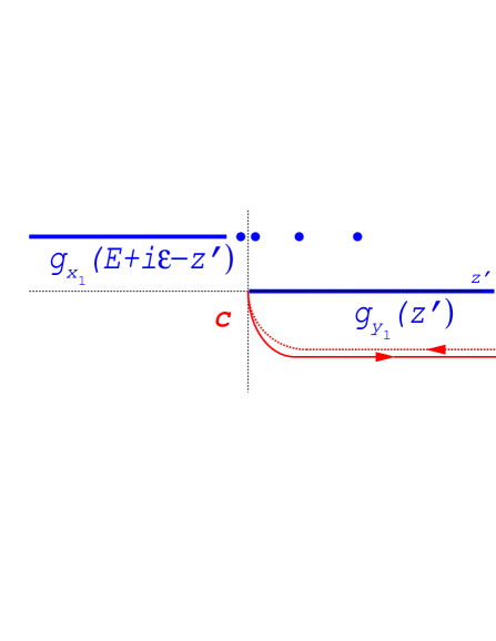
FIG. 3.: Analytic structure of $g_{x_{1}}(z-z^{\prime})\;g_{y_{1}}(z^{\prime})$ as a function of $z^{\prime}$ with $z=E+{\mathrm{i}}\varepsilon$, $E>0$, $\varepsilon>0$. The contour $C$ encircles the continuous spectrum of $h_{y_{1}}$. A part of it, which goes on the unphysical Riemann-sheet of $g_{y_{1}}$, is drawn by broken line.

$N$	$-E_{r}$	$\Gamma$
	$l_{max}=4$
20	0.058667351	0.000000133
21	0.058675722	0.000000129
22	0.058681080	0.000000127
23	0.058684499	0.000000127
24	0.058686676	0.000000127
25	0.058688060	0.000000126
	$l_{max}=5$
20	0.058702010	0.000000174
21	0.058710039	0.000000170
22	0.058715165	0.000000167
23	0.058718426	0.000000167
24	0.058720497	0.000000167
25	0.058721810	0.000000167
	$l_{max}=6$
20	0.058714400	0.000000184
21	0.058727373	0.000000180
22	0.058727373	0.000000177
23	0.058730584	0.000000177
24	0.058732621	0.000000177
25	0.058733912	0.000000177
	$l_{max}=7$
20	0.058717927	0.000000188
21	0.058725821	0.000000183
22	0.058730852	0.000000181
23	0.058734051	0.000000180
24	0.058736079	0.000000180
25	0.058737364	0.000000180
	$l_{max}=8$
20	0.058718914	0.000000190
21	0.058726801	0.000000186
22	0.058731828	0.000000183
23	0.058735023	0.000000182
24	0.058737049	0.000000183
25	0.058738333	0.000000182
	$l_{max}=9$
20	0.058719236	0.000000192
21	0.058727121	0.000000187
22	0.058732146	0.000000185
23	0.058735340	0.000000184
24	0.058737366	0.000000184
25	0.058738649	0.000000184
	$l_{max}=10$
20	0.058719374	0.000000193
21	0.058727258	0.000000189
22	0.058732283	0.000000186
23	0.058735477	0.000000185
24	0.058737503	0.000000185
25	0.058738786	0.000000185

TABLE I.: Convergence of ${}^{3}S^{e}$ 3s4s ($L=0$) positronium resonance state, b=0.25.

State	Ref. [5]		This work
${}^{1}S^{e}$	$-E_{r}$	$\Gamma$	$-E_{r}$	$\Gamma$
2s2s	0.1520608	0.000086	0.1519	0.000043
2s3s	0.12730	0.00002	0.1273	0.0000085
3s3s	0.070683	0.00015	0.0707	0.00007
3s4s	0.05969	0.00011	0.05968	0.000053
4s4s	0.04045	0.00024	0.040428	0.00013
4p4p	0.0350	0.0003	0.03502	0.00013
4s5s	0.03463	0.00034	0.03462	0.000159
5s5s	0.0258	0.00045	0.02606	0.00010
5p5p	0.02343	0.00014	0.0234	0.00004
${}^{3}S^{e}$	$-E_{r}$	$\Gamma$	$-E_{r}$	$\Gamma$
2s3s	0.12706	0.00001	0.127	0.000000003
3s4s	0.05873	0.00002	0.05874	0.0000002
4s5s	0.03415	0.00002	0.03420	0.0000007

TABLE II.: Doubly excited $L=0$ resonances of $\mbox{Ps}^{-}$. The energies and widths are expressed in Rydbergs.

REFERENCES

• [1] J. V. Noble, Phys. Rev. 161, 945 (1967).
• [2] L. D. Faddeev and S. P. Merkuriev, Quantum Scattering Theory for Several Particle Systems, (Kluver, Dordrech), (1993).
• [3] Z. Papp, C-.Y. Hu, Z. T. Hlousek, B. Kónya and S. L. Yakovlev, Phys. Rev. A, 63, 062721 (2001).
• [4] Z. Papp, I. N. Filikhin and S. L Yakovlev, Few-Body Systems, 30, 31 (2001).
• [5] Y. K. Ho, Phys. Lett., 102A, 348 (1984).
• [6] Z. Papp and W. Plessas, Phys. Rev. C, 54, 50 (1996).
• [7] R. Balian and E. Brézin, Nuovo Cim.  B 2, 403 (1969).