THE SHORT-TERM DYNAMICAL APERTURE VIA VARIATIONAL-WAVELET APPROACH WITH CONSTRAINTS

Abstract

We present the applications of wavelet analysis methods in constrained variational framework to calculation of dynamical aperture. We construct represention via exact nonlinear high-localized periodic eigenmodes expansions, which allows to control contribution to motion from each scale of underlying multiscale structure and consider qualitative approach to the problem.

1 INTRODUCTION

The estimation of dynamic aperture of accelerator is real and long standing problem. From the formal point of view the aperture is a some border between two types of dynamics: relative regular and predictable motion along of acceptable orbits or fluxes of orbits corresponding to KAM tori and stochastic motion with particle losses blown away by Arnold diffusion and/or chaotic motions. According to standard point of view this transition is being done by some analogues with map technique [1]. Consideration for aperture of n-pole Hamiltonians with kicks

$$H=\frac{p_{x}^{2}}{2}+\frac{K_{x}(s)}{2}x^{2}+\frac{p_{y}^{2}}{2}+\frac{K_{y}(s)}{2}y^{2}+$$ (1)

$$\frac{1}{3!B\rho}\frac{\partial^{2}B_{z}}{\partial x^{2}}(x^{3}-3xy^{2})L\sum_{k=-\infty}^{\infty}\delta(s-kL)+\dots$$

is done by linearisation and discretization of canonical transformation and the result resembles (pure formally) standard mapping. This leads, by using Chirikov criterion of resonance overlapping, to evaluation of aperture via amplitude of the following global harmonic representation:

$$x^{(n)}(s) = \sqrt{2J_{(n)}\beta_{x}(s)}\cdot$$

$$\cos\Big{(}\psi_{1}-\frac{2\pi\nu}{L}s+\int_{0}^{s}\frac{\mathrm{d}s^{\prime}}{\beta_{x}(s^{\prime})}\Big{)}$$

The goal of this paper is is two-fold. In part 2 we consider some qualitative criterion which is based on more realistic understanding of difference between motion in KAM regions and stochastic regions: motion in KAM regions may be described only by regular functions (without rich internal structures) but motion in stochastic regions/layers may be described by functions with internal self-similar structures, i.e. fractal type functions. Wavelet analysis approach [2], [3] provides us with more or less analytical description based on calculations of wavelet coefficients/wavelet transform asymptotics. In part 3 we consider the same problem on a more quantitative level as constrained variational problem and give explicit representation for all dynamical variables as expansions in nonlinear periodic high-localized eigenmodes.

2 QUALITATIVE ANALYSIS

Fractal or chaotic image is a function (distribution), which has structure at all underlying scales. So, such objects have additional nontrivial details on any level of resolution. But such objects cannot be represented by smooth functions, because they resemble constants at small scales [2], [3]. So, we need to find self-similarity behaviour during movement to small scales for functions describing non-regular motion. So, if we look on a “fractal” function $f$ (e.g. Weierstrass function) near an arbitrary point at different scales, we find the same function up to a scaling factor. Consider the fluctuations of such function $f$ near some point $x_{0}$

$$f_{loc}(x)=f(x_{0}+x)-f(x_{0})$$ (3)

then we have

$$f_{x_{0}}(\lambda x)\sim\lambda^{\alpha(x_{0})}f_{x_{0}}(x)$$ (4)

where $\alpha(x_{0})$ is the local scaling exponent or Hölder exponent of the function $f$ at $x_{0}$.

According to [3] general functional spaces and scales of spaces can be characterized through wavelet coefficients or wavelet transforms. Let us consider continuous wavelet transform

$$W_{g}f(b,a)=\int_{R^{n}}\mathrm{d}x\frac{1}{a^{n}}\bar{g}\left(\frac{x-b}{a}\right)f(x),$$

$b\in R^{n},\quad a>0$, w.r.t. analyzing wavelet $g$, which is strictly admissible, i.e.

$$C_{g,g}=\int_{0}^{\infty}({\mathrm{d}a}/{a})|\bar{\hat{g}(ak)}|^{2}<\infty$$

Wavelet transform has the following covariance property under action of underlying affine group:

$$W_{g}(\lambda a,x_{0}+\lambda b)\sim\lambda^{\alpha(x_{0})}W_{g}(a,x_{0}+b)$$ (5)

So, if Hölder exponent of (distribution) $f(x)$ around the point $x=x_{0}$ is $h(x_{0})\in(n,n+1)$, then we have the following behaviour of $f(x)$ around $x=x_{0}$: $f(x)=c_{0}+c_{1}(x-x_{0})+\dots+$ $c_{n}(x-x_{0})^{n}+c|x-x_{0}|^{h(x_{0})}$. Let analyzing wavelet have $n_{1}$ ($>n$) vanishing moments, then

$$W_{g}(f)(x_{0},a)=Ca^{h(x_{0})}W_{g}(f)(x_{0},a)$$ (6)

and $W_{g}(f)(x_{0},a)\sim a^{h(x_{0})}$ when $a\to 0$. But if $f\in C^{\infty}$ at least in point $x_{0}$, then $W_{g}(f)(x_{0},a)\sim a^{n_{1}}$ when $a\to 0$. This shows that localization of the wavelet coefficients at small scale is linked to local regularity. As a rule, the faster the wavelet coefficients decay, the more the analyzed function is regular. So,transition from regular motion to chaotic one may be characterised as the changing of Hölder exponent of function, which describes motion. This gives criterion of appearance of fractal behaviour and may determine,at least in principle, dynamic aperture.

3 CONSTRAINED PROBLEM FOR QUASI-PERIODIC ORBITS

We consider extension of our approach [4]-[15] to the case of constrained quasi-periodic trajectories. The equations of motion corresponding to Hamiltonian (1) may be formulated as a particular case of the general system of ordinary differential equations ${dx_{i}}/{ds}=f_{i}(x_{j},s)$, $(i,j=1,...,2n)$, where $f_{i}$ are not more than rational functions of dynamical variables $x_{j}$ and have arbitrary dependence of time but with periodic boundary conditions. Let us consider this system as an operator equation for operator $S$, which satisfies the equation

$$S(H,x,\partial/\partial s,\partial/\partial x,s)=0$$ (7)

which is polynomial/rational in $x=(x_{1}$, $\dots$ , $x_{n}$, $p_{1}$, $\dots$ , $p_{n})$ and have arbitrary dependence on $s$ and operator $C(H$, $x$, $\partial/\partial t$, $\partial/\partial x$, $s$), which is an operator describing some constraints as differential as integral on the set of dynamical variables. E.g., we may fix a part of non-destroying integrals of motion (e.g., energy) or areas in phase space (fluxes of orbits). So, we may consider our problem as constructing orbits described by Hamiltonian (1). In this way we may fix a given acceptable aperture or vice versa by feedback via parametrisation of orbits by coefficients of initial dynamical problem we may control different levels of aperture as a function of the parameters of the system (1) under consideration. As a result our variational problem is formulated for pair of operators (C, S) on extended set of dynamical variables which includes Lagrangian multipliers $\lambda$.

Then we use (weak) variation formulation

$$\int<(S+\lambda C)x,y>\mathrm{d}t=0$$ (8)

We start with hierarchical sequence of approximations spaces:

$$\dots V_{-2}\subset V_{-1}\subset V_{0}\subset V_{1}\subset V_{2}\dots,$$ (9)

and the corresponding expansions:

$$x^{N}(s)=\sum^{N}_{r=1}a_{r}\psi_{r}(s),\quad y^{N}(s)=\sum^{N}_{k=1}b_{k}\psi_{k}(s)$$ (10)

As a result we have from (7) the following reduced system of algebraical equations (RSAE) on the set of unknown coefficients $a_{i}$ of expansions (10):

$$L(S_{ij},C_{kl},a,\Lambda)=0$$ (11)

where operator L is algebraization of initial problem (7) and we need to find in general situation objects $\Lambda$.

$$\Lambda^{d_{1}d_{2}...d_{n}}_{\ell_{1}\ell_{2}...\ell_{n}}=\int\limits_{-\infty}^{\infty}\prod\psi^{d_{i}}_{\ell_{i}}(x)\mathrm{d}x,$$ (12)

We consider the procedure of their calculations in case of quasi/periodic boundary conditions in the bases of periodic wavelet functions with periods $T_{i}$ on the interval [0,T] and the corresponding expansion (10) inside our variational approach. Periodization procedure gives

$$\hat{\varphi}_{j,k}(x) \equiv \sum_{\ell\in Z}\varphi_{j,k}(x-\ell)$$ (13)

$$\hat{\psi}_{j,k}(x) \equiv \sum_{\ell\in Z}\psi_{j,k}(x-\ell)$$

So, $\hat{\varphi},\hat{\psi}$ are periodic functions on the interval [0,T]. Because $\varphi_{j,k}=\varphi_{j,k^{\prime}}$ if $k=k^{\prime}\mathrm{mod}(2^{j})$, we may consider only $0\leq k\leq 2^{j}$ and as consequence our multiresolution has the form $\displaystyle\bigcup_{j\geq 0}\hat{V}_{j}=L^{2}[0,T]$ with $\hat{V}_{j}=\mathrm{span}\{\hat{\varphi}_{j,k}\}^{2j-1}_{k=0}$ [16]. Integration by parts and periodicity gives useful relations between objects (12) in particular quadratic case $(d=d_{1}+d_{2})$:

$$\Lambda^{d_{1},d_{2}}_{k_{1},k_{2}} = (-1)^{d_{1}}\Lambda^{0,d_{2}+d_{1}}_{k_{1},k_{2}},$$ (14)

$$\Lambda^{0,d}_{k_{1},k_{2}} = \Lambda^{0,d}_{0,k_{2}-k_{1}}\equiv\Lambda^{d}_{k_{2}-k_{1}}$$

So, any 2-tuple can be represented by $\Lambda^{d}_{k}$. Then our second (after (11)) additional algebraic (linear) problem is reduced according to [16] to the eigenvalue problem for $\{\Lambda^{d}_{k}\}_{0\leq k\leq 2^{j}}$ by creating a system of $2^{j}$ homogeneous relations in $\Lambda^{d}_{k}$ and inhomogeneous equations. So, if we have dilation equation in the form $\varphi(x)=\sqrt{2}\sum_{k\in Z}h_{k}\varphi(2x-k)$, then we have the following homogeneous relations

$$\Lambda^{d}_{k}=2^{d}\sum_{m=0}^{N-1}\sum_{\ell=0}^{N-1}h_{m}h_{\ell}\Lambda^{d}_{\ell+2k-m},$$ (15)

or in such form $A\lambda^{d}=2^{d}\lambda^{d}$, where $\lambda^{d}=\{\Lambda^{d}_{k}\}_{0\leq k\leq 2^{j}}$. Inhomogeneous equations are:

$$\sum_{\ell}M_{\ell}^{d}\Lambda^{d}_{\ell}=d!2^{-j/2},$$ (16)

where objects $M_{\ell}^{d}(|\ell|\leq N-2)$ can be computed by recursive procedure

$$M_{\ell}^{d}=2^{-j(2d+1)/2}\tilde{M_{\ell}^{d}},$$ (17)

$$\tilde{M_{\ell}^{k}}=<x^{k},\varphi_{0,\ell}>=\sum_{j=0}^{k}{k\choose j}n^{k-j}M_{0}^{j},\quad\tilde{M_{0}^{\ell}}=1.$$

So, this problem is the standard linear algebraical problem.

Then, we may solve RSAE (11) and determine unknown coefficients from formal expansion (10) and therefore to obtain the solution of our initial problem. It should be noted that if we consider only truncated expansion with N terms then we have from (11) the system of $N\times 2n$ algebraical equations and the degree of this algebraical system coincides with the degree of initial differential system. As a result we obtained the following explicit representation for periodic trajectories in the base of periodized (period $T_{i}$) wavelets (10):

$$x_{i}(s)=x_{i}(0)+\sum_{k}a_{i}^{k}\psi_{k}^{i}(s),\quad x_{i}(0)=x_{i}(T_{i}),$$ (18)

Because affine group of translation and dilations is inside the approach, this method resembles the action of a microscope. We have contribution to final result from each scale of resolution from the whole infinite scale of spaces. More exactly, the closed subspace $V_{j}(j\in{\bf Z})$ corresponds to level j of resolution, or to scale j. The solution has the following form

$$x(s)=x_{N}^{slow}(s)+\sum_{j\geq N}x_{j}(\omega_{j}s),\quad\omega_{j}\sim 2^{j}$$ (19)

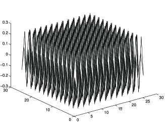
Figure 1: Periodic structure on level 6.

which corresponds to the full multiresolution expansion in all time scales. Formula (19) gives us expansion into a slow part $x_{N}^{slow}$ and fast oscillating parts for arbitrary N. So, we may move from coarse scales of resolution to the finest one for obtaining more detailed information about our dynamical process. The first term in the RHS of equation (19) corresponds on the global level of function space decomposition to resolution space and the second one to detail space. In this way we give contribution to our full solution from each scale of resolution or each time scale. On Fig. 1 we present (quasi) periodic regime on section $x-p_{x}$ corresponding to model (1).

4 ACKNOWLEDGMENTS

We would like to thank The U.S. Civilian Research & Development Foundation (CRDF) for support (Grants TGP-454, 455), which gave us the possibility to present our nine papers during PAC2001 Conference in Chicago and Ms. Camille de Walder from CRDF for her help and encouragement.

References

- [1] W. Scandale, CERN-95-06, 109; J. Gao, physics/0005023.
- [2] A. Arneodo, Wavelets, 349, Oxford, 1996.
- [3] M. Holschneider, Wavelets, Clarendon, 1998.
- [4] A.N. Fedorova and M.G. Zeitlin, Math. and Comp. in Simulation, 46, 527, 1998.
- [5] A.N. Fedorova and M.G. Zeitlin, New Applications of Nonlinear and Chaotic Dynamics in Mechanics, 31, 101 Kluwer, 1998.
-
[6]
A.N. Fedorova and M.G. Zeitlin,
CP405, 87, American Institute of Physics, 1997.
Los Alamos preprint, physics/9710035. - [7] A.N. Fedorova, M.G. Zeitlin and Z. Parsa, Proc. PAC97 2, 1502, 1505, 1508, APS/IEEE, 1998.
- [8] A.N. Fedorova, M.G. Zeitlin and Z. Parsa, Proc. EPAC98, 930, 933, Institute of Physics, 1998.
- [9] A.N. Fedorova, M.G. Zeitlin and Z. Parsa, CP468, 48, American Institute of Physics, 1999. Los Alamos preprint, physics/990262.
- [10] A.N. Fedorova, M.G. Zeitlin and Z. Parsa, CP468, 69, American Institute of Physics, 1999. Los Alamos preprint, physics/990263.
-
[11]
A.N. Fedorova and M.G. Zeitlin,
Proc. PAC99,
1614, 1617, 1620, 2900, 2903,
2906, 2909, 2912, APS/IEEE, New York, 1999.
Los Alamos preprints:
physics/9904039,
physics/9904040, physics/9904041, physics/9904042,
physics/9904043, physics/9904045, physics/9904046,
physics/9904047. - [12] A.N. Fedorova and M.G. Zeitlin, The Physics of High Brightness Beams, 235, World Scientific, 2000. Los Alamos preprint: physics/0003095.
-
[13]
A.N. Fedorova and M.G. Zeitlin, Proc. EPAC00, 415, 872, 1101, 1190, 1339, 2325 ,Austrian Acad. Sci., 2000.
Los Alamos preprints: physics/0008045, physics/0008046,
physics/0008047, physics/0008048, physics/0008049,
physics/0008050. - [14] A.N. Fedorova, M.G. Zeitlin, Proc. 20 International Linac Conf., 300, 303, SLAC, Stanford, 2000. Los Alamos preprints: physics/0008043, physics/0008200.
-
[15]
A.N. Fedorova, M.G. Zeitlin, Los Alamos preprints:
physics/0101006, physics/0101007 and World Scientific, in press. - [16] G. Schlossnagle,e.a. Technical Report ANL-93/34.