High Temperature Electron Localization in Dense He Gas

Abstract

We report new accurate mesasurements of the mobility of excess electrons in high density Helium gas in extended ranges of temperature $[(26\leq T\leq 77)\,{K}]$ and density $[(0.05\leq N\leq 12.0)$ ${atoms}\cdot{nm}^{-3}]$ to ascertain the effect of temperature on the formation and dynamics of localized electron states. The main result of the experiment is that the formation of localized states essentially depends on the relative balance of fluid dilation energy, repulsive electron–atom interaction energy, and thermal energy. As a consequence, the onset of localization depends on the medium disorder through gas temperature and density. It appears that the transition from delocalized to localized states shifts to larger densities as the temperature is increased. This behavior can be understood in terms of a simple model of electron self–trapping in a spherically symmetric square well.

I Introduction

The transport properties of excess electrons in dense noble gases and liquids give useful information on the electron states in a disordered medium and on the relationship between the electron–atom interaction and the properties of the fluid. The electron behavior depends on the strength of its coupling with the gas atoms and on the response function of the gas itself. Therefore, different transport mechanisms and regimes can be obtained according to the nature of the electron–atom interaction (repulsive or attractive), to the thermodynamic conditions of the gas, either close to or removed from its critical point, and to the amount of disorder inherent to the fluid hern91 .

Typically, at low density and high temperature, electrons are quasifree. Their wavefunction is pretty delocalized and the resulting mobility is large. They scatter elastically off the atoms of noble gases in a series of binary collisions and the scattering process is basically determined by the interaction potential through the electron–atom scattering cross section. The mobility can be predicted accurately by the classical kinetic theory hux74 .

At higher densities, and, possibly, at lower temperatures, electrons may either remain quasifree with large mobility (as in the case of Argon), or they can give origin to a new type of state that is spatially localized inside a dilation of the fluid. In this case the mobility is very low because the complex electron plus fluid dilation moves as an unique, massive entity. This, for instance, happens in He and Ne. The main difference between the two cases is that in the former the electron–atom interaction is attractive (Ar) and in the latter is repulsive (He and Ne) borg941 ; borg942 .

The simplest model to describe the behavior of electrons in a dense, disordered medium is the hard–sphere gas and a practical realization of this system is represented by He. In He the electron–atom interaction is pretty well described by a hard–core potential and the scattering cross section is fairly large and energy independent. It is well known that the charge transport proceeds via bubble formation in liquid He at low temperature levi ; harri ; sch80 ; ja . In gaseous He at low temperature the mobility shows a drop of several orders of magnitude when the density is increased from low to medium values. This drop has been intepreted in terms of a continuous transition from a transport regime where the excess electrons are quasifree to a region where they are localized. There is still controversy about the nature of the localized states, whether they are localized in bubbles as in the case of the liquid or whether they are localized in the Anderson sense poli . In this case the electron wavefunction decays exponentially with the distance owing to multiple scattering effects induced by the disorder of the medium om .

Owing to these considerations, it is interesting to investigate the localization transition at higher temperatures. Therefore, we have measured the mobility of excess electrons in dense He gas at temperatures $26<T<77\,K.$ By assuming that electrons are localized in dilations of the gas, a simple quantum mechanical model provides a good semiquantitative description of the observed behavior of the mobility.

II Experimental Details

The mobility measurements have been carried out by using a swarm technique in a Pulsed Townsend Photoinjection apparatus we have been exploiting for a long time for electron and ion mobility measurements borg88 ; borg90 ; borg93 . A schematics of the apparatus is shown in Figure 1.

Figure 1: Schematics of the experimental apparatus. See the text for a description.

Briefly, a high-pressure cell (CN), that can withstand pressures up to 10 MPa, is mounted on the cold head of a cryocooler inside a triple-shield thermostat. The cell is operated between 25 and 330 K. Temperature is stabilized within 0.01 K.

A parallel-plate capacitor, consisting of an emitter (E) and a collector (C), is contained in the high-pressure cell and is energized by the high-voltage generator -V. A digital voltmeter (DV) reads the voltage. The distance between the two plates delimits the drift space. An electron swarm is produced by irradiating the gold-coated quartz window placed in the emitter with the VUV light pulse of a Xe flashlamp (FL). The amount of produced charge ranges between 4 and 400 fC, depending on the gas pressure and on the applied electrical field strength. Under its action, the charges drift towards the anode inducing a current in the external circuit. The current is integrated by the analog circuit RC in order to improve the signal-to-noise ratio. Two different operational amplifiers (SA and FA) are used depending on the duration of the signal. This is recorded by a high-speed digital transient analyzer (DS) and is fetched by a personal computer for the analysis of the waveform.

Ultra-high purity He gas with an impurity content, essentially Oxygen, of some p.p.m is used. The impurity content is reduced to a few p.p.b. by circulating the gas in a recirculation loop driven by a home-made bellow circulator (BC) that forces the gas to be purified through an Oxisorb cartridge (OX) and a LN2-cooled active-charcoal trap (CT).

The induced signal waveform of the electron drifting at constant speed is a straight line, and the drift time is easily determined by the analysis of the waveform. The overall accuracy of the mobility measurements is $|\Delta\mu/\mu|\approx 5\,\%.$

III Experimental Results

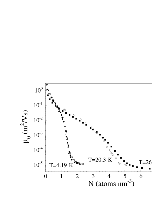
Figure 2: Experimental zero–field mobility $\mu_{0}$ as a function of the gas density. $T=26\,K:$ present work; $T<26K:$ literature data at $T\approx 4\,K$ levi ; harri ; sch80 and at $T\approx 20\,K$ ja .

In Figure 2 we show the observed zero–field mobility $\mu_{0}$ in He at $T\approx 26\,K.$ The present data are compared with literature data for $T=4.2\,K$ levi ; harri ; sch80 and for $T=20.3\,K$ ja . At $T=26\,K$ $\mu_{0}$ exhibits the same qualitative behavior observed earlier at much lower temperatures. As the gas density increases, $\mu_{0}$ decreases by nearly 5 orders of magnitude. The continuous transition from the low–density high–mobility region is interpreted as the progressive depletion of extended or delocalized states and the consequent formation of localized states poli ; iaku1 . These are assumed to consist of an electron trapped into a cavity in the fluid. This cavity is referred to as an electronic bubble. A similar physical process has been observed also in liquid bruschi and gaseous Neon borg90 . In gaseous Neon, the $\mu_{0}$ data resemble closely those shown in Figure 2 and the interpretation of the Neon data, as due to electron localization in cavities, has been confirmed by quantum–mechanical Molecular Dynamics calculations ancilotto .

The dynamics of the localization process, though not investigated experimentally, is quite clear rose1 ; rose2 ; sakai . However, even if the localization process were of the Anderson type poli , i.e., electrons with energy below the mobility edge trapped as a consequence of the self–interference of their wavefunction because of the medium disorder, nonetheless electrons wind up by forming electron bubbles because of the repulsive electron–medium interaction and medium compliance. The existence of such bubbles has been also confirmed experimentally by infrared absorption spectra in liquid He adams1 ; adams2 .

Once all of the electron states are localized, the resulting $\mu_{0}$ is not zero because the gas is compliant enough to allow the large complex structure made of an electron plus the associated bubble to diffuse slowly hern91 and drift under the action of an external electric field..

The main difference between the present data and those at lower temperatures is that the transition to low mobility states is shifted to larger values of the density. At $T=4.2\,K$ the transition can be considered complete at a density $N\approx 2\,atoms\cdot nm^{-3}.$ At $T\approx 20.3\,K$ the final state is reached for $N\approx 4.8\,atoms\cdot nm^{-3},$ while at $T=26\,K$ in our experiment this density has moved to $N\approx 6.2\,atoms\cdot nm^{-3}.$ This is even more evident at higher temperatures.

It is evident that the formation of localized states is not related to the presence of a nearby critical point (the critical temperature of He is $T_{c}\approx 5.2\,K).$ It rather seems related to the competition between the thermal energy of electrons and the free energy of localization. Therefore, it appears reasonable that the localization transition shifts at larger densities for higher temperatures in order to achieve increasingly larger free energies.

The localization transition can be noticed also by observing the electric field dependence of the mobility.

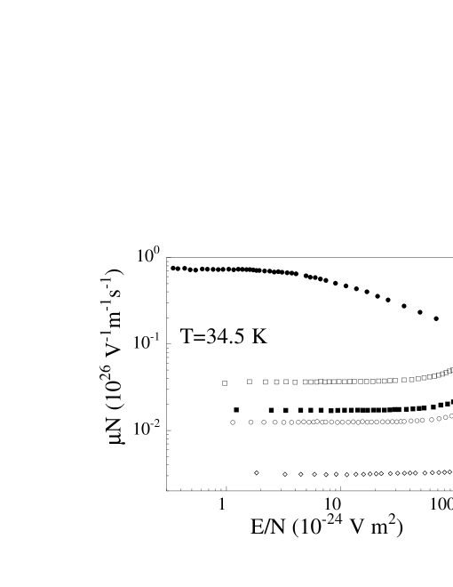
Figure 3: Density–normalized mobility $\mu N$ as a function of the reduced electric field $E/N$ at $T=34.5\,K$ for several densities: $N=0.154,\,4.174,\,4.658,$ $4.833,\,5.558\,atoms\cdot nm^{-3}$ (from top).

In Figure 3 we plot the density–normalized mobility $\mu N$ as a function of the reduced field $E/N$ at $T=34.5\,K$ for several densities. The behavior at different temperatures is similar to this one.

At small $N$ and low $E/N,$ electrons are in near thermal equilibrium with the gas atoms and $\mu N$ is constant. As $E/N$ increases, $\mu N$ decreases, eventually reaching the $(E/N)^{-1/2}$ dependence expected on the basis of the classical kinetic theory because the scattering rate increases with the electron kinetic energy hux74 .

At high $N,$ $\mu N$ is very low and practically independent of E/$N,$ at least for the highest electric fields of the present experiment (up to $\approx 7\,kV/cm$). At such densities, almost all of the electrons are localized in bubbles. Even the highest electric field reached in the experiment is not large enough to heat up such massive objects. The electronic bubbles therefore remain in equilibrium with the gas atoms.

At intermediate values of $N,$ the behavior of $\mu N$ is quite complicated. At small $E/N,$ $\mu N$ is constant, while at larger $E/N,$ $\mu N$ reaches a maximum and finally, at even larger $E/N,$ it meets the classical $(E/N)^{-1/2}$ behavior. The same superlinear behavior of the drift velocity of electrons in dense He gas was observed also at very low temperatures sch80 .

This behavior can be interpreted in terms of the formation, at large $N,$ of electron states which are self–trapped in partially filled bubbles. These are very massive and have low mobility. By increasing the electric field strength bubbles may be either destroyed or their formation may be inhibited, so that electrons are again free and very mobile. The same behavior of $\mu N$ as a function of $E/N$ has been observed also in Neon gas and the same interpretation of the data has proven successful borg90 .

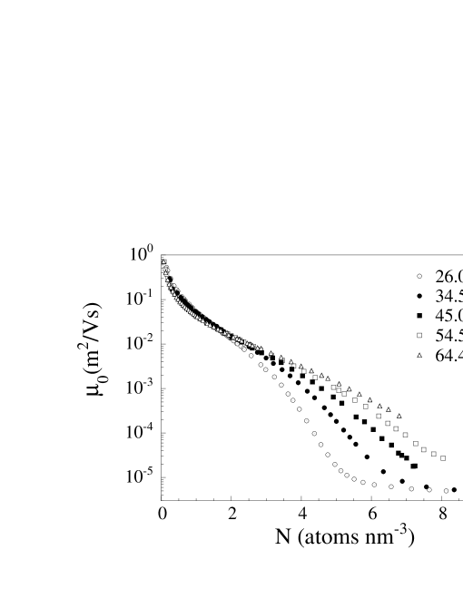
Figure 4: Zero–field mobility $\mu_{0}$ as a function of $N$ for $T=26,\,34.5,\,45.0$ $54.5,\,64.4\,K.$

In Figure 4, the zero–field value $\mu_{0}$ of the mobility $\mu$ is shown as a function of the density $N$ for the investigated temperatures. In this Figure the shift of the localization transition to larger $N$ for increasing $T$ is clearly shown. For $T>45\,K$ the transition has not been tracked down completely because the pressure required to reach such large $N$ values exceeds the capacity of our apparatus $(P\leq 10.0\,MPa.)$ Nonetheless, it is evident that the localization phenomenon occurs also at high temperatures provided that the density is large enough.

IV Discussion

A description of the observed behavior of $\mu_{0}N$ as a function of $N$ is very difficult. In fact, it must deal with the mobility of the two charge carriers, the extended and the localized electron, and also it must treat correctly the probability of occupation of the two states as a function of the density.

Moreover, although the mobility of the localized electron, i.e., of the bubble, is rather well described by the simple Stokes hydrodynamic formula, $\mu_{0}=e/6\pi\eta R,$ where $\eta$ is the gas viscosity and $R$ is the bubble radius iaku1 ; ec , the description of the mobility of the extended electron states is still rather controversial, also because the localization transition is not as sharp as desired, as, for instance, in the case of Ne borg90 .

Several theoretical models for the description of the quasifree electron mobility in dense noble gases have been devised on the basis of the Boltzmann formalism of kinetic theory borg941 ; poli ; om . Their common feature is the realization that multiple scattering effects concur to dress the electron–atom scattering cross section. It has also been suggested ioffe that, when the ratio between the electron thermal wavelength $\lambda_{T}$ and its mean free path $\ell_{c}$ is $\lambda_{T}/\ell_{c}\approx 1,$ the scattering rate diverges poli and electrons get localized as a consequence of the interference of two scattering processes: the scattering off several different scattering centers and the time–reversed scattering sequence asca . This model naturally introduces a mobility edge, an energy below which the electron wavefunction does not propagate.

Although this mobility–edge model describes well the electron mobility in dense He gas, it has two main drawbacks. The first one is that it works correctly only for He, because its scattering cross section is large and nearly energy independent. For Ne, for instance, it does not correctly describe the experimental data because of the strong dependence of the momentum transfer scattering cross section borg92 .

Moreover, it is well known that, in liquid He, electrons trapped in stable cavities within the fluid have been observed by IR spectroscopy adams1 ; adams2 ; hern91 and this observation has been confirmed also by quantum–mechanical Molecular Dynamics calculations kalia , while the localized states, described in the mobility–edge model as those with energy below the mobility edge, are only not propagating but do not reside in cavities. Even a static disorder produces localized electrons in this model. It is of course possible that after localization electrons could deform the fluid to produce bubble states, but the observed drop of mobility is not due to bubble formation poli .

In view of these considerations, we adopt a simple model miya that describes the formation of the self–trapped electron states as a process of localization in a quantum well. The mobility of the quasifree electrons is treated in terms of a different, heuristic model developed in our laboratory that encompasses the several multiple scattering effects present in the scattering process of an excess electron in a dense gas. We use such a model because it has given excellent agreement with the experimental data in Ne borg88 ; borg90 as well as in Ar bsl .

In addition to the usual thermal energy, electrons in the propagating state have a ground state energy $V_{0}(N)$ which depends on the density of the environment. $V_{0}(N)$ consists of two contributions sjc

$$V_{0}(N)=E_{K}(N)+U_{P}(N)$$ (1)

$U_{P}$ is a negative potential energy term arising from the screened polarization interaction of electrons with the gas atoms. $E_{K}(N)$ is a positive kinetic energy contribution due to excluded volume, quantum effects.

Owing to the small He polarizability, $U_{P}$ can be neglected thus yielding $V_{0}\approx E_{K}.$ It has been shown borg90 ; bsl ; broomall that $E_{K}$ is quite accurately given by the Wigner–Seitz model

$$V_{0}=\frac{\hbar^{2}k_{0}^{2}}{2m},\quad\tan\left[k_{0}\left(r_{s}-\tilde{a}\right)\right]=k_{0}r_{s}$$ (2)

as shown in Figure 5.

Figure 5: Ground state energy $V_{0}(N)$ of a quasifree electron as a function of the gas density.

In Eq. 2, $r_{s}=(3/4\pi N)^{1/3}$ is the Wigner–Seitz radius, $\tilde{a}$ is the electron-atom scattering length, and $k_{0}$ is the ground state momentum of the electron. Owing to the fact that the electron–atom interaction is essentially repulsive, $V_{0}(N)$ is positive and increase monotonically with $N.$ This means that the lower is the gas density the lower is the ground state energy of a quasifree electron.

Since thermally activated fluctuations of the density are present, also $V_{0}$ fluctuates and electrons can get temporarily localized in a virtual or resonant state above one such density fluctuation where the local density is lower than the average one hern91 ; merz .

If the electron–atom interaction is strongly enough repulsive (as in the case of He) and if the fluctuation is sufficiently deep, there can be formation of a self–trapped electron state, whose stability can be determined by minimizing its free energy with respect to the quasifree state.

We therefore assume that localized electron resides in a quantum square well of spherical simmetry. The well radius is $R.$

Since the gas has no surface tension and since the temperature is pretty high for He atoms to have significant thermal energy, we must allow for some He atoms penetrating into the cavity and dynamically interchanging with outside atoms. We thus assume the bubble to be partially filled with density $N_{i}<N$ and filling fraction $F=N_{i}/N.$ The electron is thus subjected to the following spherically symmetric potential

$$\left\{\begin{array}[]{cc}V_{i}&\mbox{for }r<R\\ V_{0}&\mbox{for }r\geq R\end{array}\right.$$

where $V_{i}$ is defined as the ground state energy of an electron inside the bubble. Since $N_{i}<N,$ $V_{i}<V_{0}.$ The potential inside the bubble must take into account also the contribution of the polarization energy due to the outside gas. If the bubble were empty, the polarization energy ${\cal E}_{P}$ could be written as miya

$${\cal E}_{P}=-\frac{\alpha e^{2}}{2(4\pi\epsilon_{0}R)}N$$ (3)

Since the bubble is only partially empty, to first order the polarization energy contribution can be written as borg90

$${\cal E}_{P}=-\frac{\alpha e^{2}}{2(4\pi\epsilon_{0}R)}(1-F)N$$ (4)

In this case the potential energy of the electron inside the bubble can be cast in the form

$$V_{i}=V_{F}+{\cal E}_{P}$$ (5)

with $V_{F}=V_{0}(FN),$ i.e., the $V_{0}$ value at the density of the interior of the bubble.

A solution of the Schrődinger equation is sought for the lowest bound $s$–wave state, if it exists, of energy eigenvalue ${\cal E}_{1}.$ Only the first eigenvalue is relevant because the temperature is quite low. If ${\cal R}(r)$ is the ground state solution of the radial Schrődinger equation, the function $f(r)=r{\cal R}(r)$ fulfills the radial equation

$$\begin{array}[]{ccc}\left[{\frac{{\rm d}^{2}}{{\rm d}r^{2}}}+k_{i}^{2}\right]f(r)=0&\mbox{for}&r<R\\ \left[{\frac{{\rm d}^{2}}{{\rm d}r^{2}}}-k_{o}^{2}\right]f(r)=0&\mbox{for}&r\geq R\end{array}$$

where $k_{i}^{2}=(2m/\hbar^{2})({\cal E}_{1}-V_{i})$ and $k_{o}^{2}=(2m/\hbar^{2})(V_{0}-{\cal E}_{1}).$ By imposing the boundary conditions on the radial wavefunction at the bubble boundary for $r=R,$ we obtain the eigenvalue equation

$$-\tan{X}={\frac{X}{\left(H^{2}-X^{2}\right)^{1/2}}}$$ (6)

with $X=k_{i}R$ and $H^{2}=(2m/\hbar^{2})(V_{0}-V_{i})R^{2}.$ If $X_{1}$ is the solution of Eq. 6, then the energy ${\cal E}_{1}$ of the $s-$wave state is

$${\cal E}_{1}=\frac{\hbar^{2}}{2mR^{2}}X_{1}^{2}+V_{i}$$ (7)

The Schrődinger equation admits solutions if the well strength is such that $H^{2}\geq\pi^{2}/4.$ This translates into a condition on a minimum bubble radius for the existence of a solution, namely

$$R_{0}^{2}=\frac{\hbar^{2}\pi^{2}}{8m\left(V_{0}-V_{i}\right)}$$ (8)

For each value $R>R_{0}$ the eigenvalue equation Eq. 6 is solved for $X_{1},$ and the eigenvalue ${\cal E}_{1}$ is calculated from Eq. 7 as a function of the gas density and of the filling fraction of the bubble.

In Figure 6 we show the shape of a typical $s-$ wave solution of the Schrődinger equation.

Figure 6: Radial probability density for the $s-$wave ground state in the partially empty spherically symmetric square well.

The excess free energy of the localized state with respect to the delocalized one can be computed as

$$\Delta{\cal F}={\cal E}_{1}+V_{i}+W-V_{0}$$ (9)

where $W$ is the volume work, at constant $T,$ required to expand the bubble and is given by borg90

$$W={\frac{4\pi}{3}}R^{3}P\Bigl{[}1-F-{FN\over P}\int\limits_{FN}^{N}{P\over n^{2}}{\rm d}n\Bigr{]}$$ (10)

$P$ is the gas pressure. In order to find the most probable state, $\Delta{\cal F}$ is minimized with respect to the bubble radius and filling fraction. Rigorously speaking, the minimum excess free energy should be obtained by averaging $\Delta{\cal F}$ over all atomic configurations leading to trapped electron states. This is a formidable task and therefore, to a first approximation, we adopt the optimum atom–concentration fluctuation iaku1 , i.e., that which causes the largest decrease of the system free energy as a consequence of electron trapping.

In Figure 7 we show the free energy of the localized state ${\cal E}_{1}+V_{i}+W$ as a function of the bubble radius at fixed $T=64\,K$ and $N=7.8\,atoms\cdot nm^{-3}$ for several filling fraction values.

Figure 7: Free energy of the localized state for given $T=64\,K$ and $N=7.8\,atoms\cdot nm^{-3}$ for filling fraction $F=0,\,0.1,\,0.2,\,0.3,\,0.4,\,0.5,\,0.6$ as a function of the bubble radius.

Once minimized as a function of the bubble radius, this first minimum value of excess free energy is plotted in Figure 8 as a function of the filling fraction for several $N$ at fixed temperature.

For smaller densities, this excess free energy minimized with respect to bubble radius at constant $N$ and $T$ is a monotonically decreasing function of the filling fraction $F.$ This means that the incipient bubble is not stable. It gets more and more filled until it disappears completely.

Figure 8: The excess free energy, minimized with respect to the bubble radius, as a function of the filling fraction for $5,\,5.3,\,5.5,\,5.7,\,6,\,6.3,\,6.5,\,6.8\,atoms\cdot nm^{-3}.$ for $T=64.4\,K$ (from top).

Stable states are now sought by carrying out a second minimization of excess free energy as a function of the filling fraction $F.$

This double minimization procedure finally yields the optimum values of filling fraction $F_{B}$ and bubble radius $R_{B},$ shown in Figure 9 for $T=26\,K$ as a function of the gas density.

It can be seen that, at constant $T,$ bubbles tend to become smaller and emptier as the density increases. The optimum bubble radius is $R_{B}\approx 1.5-2\,\,nm,$ compatible with the observed values in liquid He hern91 .

Figure 9: Optimum equilibrium filling fraction $F_{B}$ and radius $R_{B}$ of the electron bubble for $T=26\,K$ as a function of the density.

The values of the excess free energy corresponding to the optimum filling fraction and bubble, $\Delta F_{B}=\Delta F(R_{B},F_{B},N,T),$ are reported in Figure 10.

Bubble states start forming as soon as $\Delta{\cal F}_{B}=0,$ but they are not stable against thermal fluctuations until $|\Delta{\cal F}_{B}/k_{{B}}T|\gg 1.$ For a given $T,$ this condition is fulfilled only if $N$ is large enough. Moreover, by inspecting Fig. 10, we see that a given value of $\Delta{\cal F}_{B}$ is obtained at increasingly higher densities as the temperature is increased.

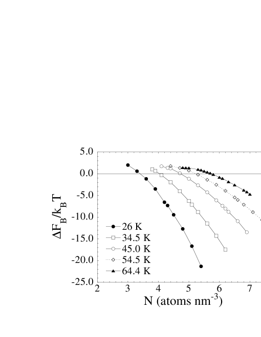
Figure 10: Minimum excess free energy of the localized state as a function of $N$ for several $T.$

Figure 11: Density values $N^{\star}$ where localized and delocalized states are equiprobable as a function of $T.$

In Figure 11 we show the values of density $N^{\star}$ where $\Delta{\cal F}_{B}=0.$ At this density the localized and delocalized states are equiprobable. In agreement with the experimental observation on mobility, $N^{\star}$ increases with $T.$ This means that bubbles become stable at larger $N$ when $T$ increases, both because electrons have more thermal energy and because the volume work to expand the bubble increases with the temperature.

Once the minimum excess free energy has been computed, the fraction of bubble and quasifree states is readily calculated as $n_{B}/n_{F}=\exp{\{-\Delta{\cal F}_{B}\}}.$ The observed mobility is then a weighted sum of the contribution of the mobilities of the two states iaku1 ; young . For the bubble state the semihydrodynamic mobility

$$\mu_{B}=\frac{e}{6\pi\eta R_{B}}\left[1+\frac{9\pi\eta}{4NR_{B}(2\pi mk_{{B}}T)^{1/2}}\right]$$ (11)

has been used ec , where $\eta$ is the gas viscosity wasserman .

For the mobility of the quasifree states we have used the results of the heuristic Padua model, succesfully exploited in Ne borg88 ; borg90 and Ar bsl . The quasifree electron mobility can be written as hernmart

$$\mu_{F}=\frac{4e}{3hS(0)}\lambda_{T}\lambda^{\star}\exp{\left(-\lambda_{T}/\sqrt{\pi}\lambda^{\star}\right)}$$ (12)

where $h$ is the Planck’s constant. $S(0)=Nk_{B}T\chi_{T}$ is the long–wavelength limit of the static structure factor and $\chi_{T}$ is the gas isothermal compressibility. $\lambda_{T}=h/\sqrt{2\pi mk_{B}T}$ is the thermal wavelength of the electron. Finally, $\lambda^{\star}$ is defined as

$$\lambda^{\star}=\frac{1}{N}\left(k_{B}T\right)^{2}\int\limits_{0}^{\infty}\frac{\epsilon}{\sigma_{mt}\left(\epsilon+E_{k}\right)}{\rm e}^{\left(-\epsilon/k_{B}T\right)}{\rm d}\epsilon$$ (13)

where $\sigma_{mt}(\epsilon+E_{k})$ is the momentum transfer scattering cross section evaluated at the electron energy shifted by the kinetic contribution $E_{k}$ of the ground state energy shift $V_{0}.$ We recall here that, for He, $E_{k}\approx V_{0}.$ The exponential factor in Equation 12 is due to O’Malley om . This model includes the three main effects of multiple scattering bsl :

• the shift $V_{0}$ of the ground state energy of a quasifree electron in a medium of density $N;$

• the correlation among scatterers taken into account by the static structure factor $S(0)$ lekner ;

• the increase of the scattering rate due to quantum self–interference of electron multiply scattered in a time reversed sequence by the same scattering centers asca and described by the O’Malley factor in Eq. 12.

Figure 12: Zero–field mobility $\mu_{0}$ vs. $N$ for $T=26\,{K}.$ The solid line is the mobility of quasifree electron states. The dashed line is the weighted average mobility.

In Figure 12 we show the results of the model for $T=26\,K.$ The quasifree mobility in the low–density side is well described by the heuristic model and also the density where the localization transition occurs is reproduced with satisfactory accuracy. Similar results are obtained for the higher temperatures.

In Figure 13 we show the experimental mobility in the high–density region for $26<T<64\,K$ with the average mobility at high density calculated according to the model.

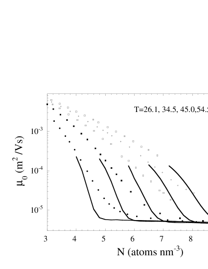
Figure 13: Zero–field mobility $\mu_{0}$ vs. $N$ for $T=26.1,\,34.5,\,45.0,\,54.5,\,64.4\,{K}$ in the high–density region. The solid line is the calculated average mobility.

This Figure clearly shows that the present model quite accurately predicts the shift of the localization transition to higher densities when the temperature is increased, although it does not fit the data with great accuracy.

V Conclusions

The electron mobility in dense He gas shows two distinct regimes at low and high $N.$ At low $N$ the states of the excess electrons are extended, while at high $N$ electrons are localized in bubbles. Both states are present at all $N,$ but bubble states become stable, at fixed $T,$ only if $N$ exceeds a certain value $N^{\star}.$ The measured mobility is a weighted sum of the contribution of the two kind of electrons, quasifree and localized.

A simple model of electron localization in a quantum square well explains the observed fact that the localization transition shifts to higher $N$ as $T$ increases. It also semiquantitatively describes the observed mobility. The agreement of the model with the data, however, is far from satisfactory. More sophisticated models, namely those based on the so–called self–consistent–field approximation iaku1 ; hernmart2 , where the density profile of the bubble is self–consistently calculated along with the electron wavefunction, can be used with results not very different from the present ones.

Among possible reasons to explain the discrepancy of the present model with the experimental data, there could be the fact that the bubble model is a simple two–state model and neglects the possibility that bubbles have a distribution of radii and filling fractions. Moreover, even the description of mobility of the quasifree electrons is not yet completely satisfactory.

References

- (1) J.P.Hernandez, Rev. Mod. Phys., 63, 675 (1991).
- (2) L.G.Huxley and R.W.Crompton, The Diffusion and Drift of Electrons in Gases (Wiley, New York, 1974).
- (3) A.F.Borghesani and M.Santini, in Linking the Gaseous and Condensed Phases of Matter. The Behavior of Slow Electrons, L.G.Christophorou, E.Illenberger, and W.F. Schmidt Editors, NATO ASI Series, Vol. B 326 (Plenum, New York, 1994), pp. 259–279.
- (4) A.F.Borghesani and M.Santini, in Linking the Gaseous and Condensed Phases of Matter. The Behavior of Slow Electrons, L.G.Christophorou, E.Illenberger, and W.F. Schmidt Editors, NATO ASI Series, Vol. B 326 (Plenum, New York, 1994), pp. 281–301.
- (5) J.L.Levine and T.M.Sanders, Phys. Rev. 154, 138 (1967).
- (6) H.R.Harrison, L.M.Sander, and B.E.Springett, Phys. Rev. B 6, 908 (1973).
- (7) K.W.Schwarz, Phys. Rev. B 21, 5125 (1980).
- (8) J.A.Jahnke, M.Silver, and J.P.Hernandez, Phys. Rev. B 12, 3420 (1975).
- (9) A.Ya.Polishuk, Physica 124 C, 91 (1984).
- (10) T.F.O’Malley, J. Phys. B 13, 1491 (1980).
- (11) A.F.Borghesani, L.Bruschi, M.Santini, and G.Torzo, Phys. Rev. A 37, 4828 (1988).
- (12) A.F.Borghesani and M.Santini, Phys. Rev. A 42, 7377 (1990).
- (13) 30. A.F.Borghesani, D.Neri, and M.Santini, Phys. Rev., E 48, 1379 (1993).
- (14) A.G.Khrapak and I.T. Yakubov, Sov. Phys. Usp. 22, 703 (1979).
- (15) L.Bruschi, G.Mazzi, and M.Santini, Phys. Rev. Lett. 28, 1504 (1972).
- (16) F. Ancilotto and F.Toigo, Phys. Rev. A 45, 4015 (1992).
- (17) M.Rosenblit and J.Jortner, Phys. Rev. Lett. 75, 4079 (1995).
- (18) M.Rosenblit and J.Jortner, J. Phys. Chem. 101, 751 (1997).
- (19) Y.Sakai, A.G.Khrapak, and W.F.Schmidt, Chem. Phys. 164, 139 (1992).
- (20) C.C.Grimes and G.Adams, Phys. Rev. B 41, 6366 (1990)
- (21) C.C.Grimes and G.Adams, Phys. Rev. B 45, 2305 (1992)
- (22) A.Nakano, P.Vashishta, R.K.Kalia, Phys. Rev. B 43, 10928 (1991).
- (23) T.P.Eggarter and M.H.Cohen, Phys. Rev. Lett. 27, 129 (1971).
- (24) A.F.Ioffe and A.R.Regel, Prog. Semicond. 4, 237 (1960).
- (25) G.Ascarelli, Phys. Rev. B 33, 5825 (1986).
- (26) A.F.Borghesani and M.Santini, Phys. Rev. A 45, 8803 (1992).
- (27) T.Miyakawa and D.L.Dexter, Phys.Rev. 184, 166 (1969).
- (28) A.F.Borghesani, M.Santini, and P.Lamp, Phys. Rev. A 46, 7902 (1992).
- (29) B.E.Springett, J.Jortner, and M.H.Cohen, J. Chem. Phys. 48, 2720 (1968).
- (30) J.R.broomall, W.D.Johnson, and D.G.Onn, Phys. Rev. B 14, 2819 (1976).
- (31) E.Merzbacher, Quantum Mechanics (Wiley, New York, 1970).
- (32) R.A.Young, Phys. Rev. A 2, 1983 (1970).
- (33) V.V.Sychev, A.A.Vasserman, A.D.Kolzov, G.A.Spiridonov, and V.A.Tsymarny, Thermodynamic Properties of Helium (Springer, Berlin, 1987).
- (34) J.P.Hernandez and L.W.Martin, Phys. Rev. A 43, 4568 (1991).
- (35) J.Lekner, Philos. Mag 18, 1281 (1972).
- (36) J.P.hernandez and L.W.Martin, J. Phys.:Condensed Matter 4, L1 (1992).