Optical absorption in a degenerate Bose gas

Abstract

We here develop a theory on optical absorption in a dilute Bose gas at low temperatures. This theory is motivated by the Bogoliubov theory of elementary excitations for this system, and takes into account explicitly the modification of the nature and dispersion of elementary excitations due to Bose-Einstein condensation. Our results show important differences from existing theories.

PACS numbers: 03.75.Fi, 32.70.Jz, 32.80.-t

A remarkable property of a degenerate Bose gas is the modification of the nature of excitations in the system. This has been elucidated by the work of Feymann and Bogoliubov [1]. For a classical or non-degenerate Bose gas, elementary excitations are basically quasiparticles. For a degenerate Bose gas however, the long wavelength elementary excitations are the same as density waves of the system, propagating at the sound velocity. They correspond to neither addition nor removal of a quasiparticle, but a linear combination of both. At short wavelengths these excitations resemble more closely quasiparticles, with the dispersion the same as free particles apart from a shift.

Recently there is much interest in optical excitations in dilute degenerate Bose gas. The frequency of absorption has been used as an indication of the formation of Bose-Einstein condensation in the system [2]. An optical excitation is a non-trivial process, as one of the original atoms (referred to as a-atoms below), all identical before the excitation occurs, is converted to another one which is distinguishable from all the others. Moreover a-atoms which are not excited internally interact differently with this ‘foreign’ atom (referred to as c-atom below) than among themselves, and must respond by rearrangement of their relative motion. The frequencies at which optical absorption occur are therefore different from $\omega_{0}$, the value for a single isolated atom.

Optical absorption in a Bose gas has been considered by Oktel and Levitov [3], and also by Pethick and Stoof [4]. Johnsen and Kavoulakis [5] considered the case of excitons in semiconductors where the initial and final bosons have different effective masses, using an approximation equivalent to that used by Oktel and Levitov [3]. Let us briefly summarize the main results of Ref. [3] most relevant to the discussions below. These authors concentrate on intermediate to high temperatures and ignore the modifications of the nature of quasiparticles below the transition temperature. They make the dramatic prediction that, for $T<T_{c}$ and in the limit of no momentum transfer, there is actually not one but two absorption lines. These lines are located at the frequencies

$$\omega=\omega_{0}+g_{ac}n-g_{aa}(n_{0}+2n_{T})+y$$ (1)

where $y$ obeys the quadratic equation $y(y-g_{ac}n_{T}+g_{aa}n_{0})=g_{ac}^{2}n_{0}n_{T}$. Here $g_{aa}$ and $g_{ac}$ are the interaction parameters among the a-atoms and between c- and a-atoms respectively, $n_{0}$ the number density of the condensate and $n_{T}$ that of the thermal atoms, $n=n_{0}+n_{T}$ the total number density. As $T\to 0$, $y\to 0$ and $-g_{aa}n$ though the weight of the second line also approaches zero. For $T\to T_{c}$, $y\to 0$ and $y\to g_{ac}n$ with the weight of the first line vanishing. Note then the second solution of $y$ then yields the line $\omega=\omega_{0}+2(g_{ac}-g_{aa})n$.

Here we would like to re-examine and extend this investigation to low temperatures. In particular, we are interested in the effects brought about by the macroscopic occupation of the lowest energy state. Note that not only the dispersion is changed for $T<T_{c}$, but also that now the annihilation of an a-atom can correspond both to an absorption and a creation of a Bogoliubov excitation. We shall see that properly accounting for these features substantially modifies the absorption spectrum. In general it no longer simply consists of two lines. In some regimes where the spectrum is approximately two relatively sharp lines, the frequencies of these lines differ from those of eq (1).

We then consider a weakly interacting Bose gas. The Hamiltonian of this system is given by

$$H_{a}=\sum_{p}\xi_{p}a^{\dagger}_{p}a_{p}+{g_{aa}\over 2V}\sum^{\prime}a^{\dagger}_{p1}a^{\dagger}_{p2}a_{p3}a_{p4}$$ (2)

Here $\xi_{p}=p^{2}/2m$ is the kinetic energy of a free a-boson of momentum $p$ (we shall drop all vector labels since no confusion will arise), and the second sum is over $p$’s with the constraint $p_{1}+p_{2}=p_{3}+p_{4}$. $V$ is the volume. The Hamiltonian of the system containing also a c-atom is given by $H=H_{a}+H_{c}+H_{ac}$. $H_{c}$ describes the free motion of the c-atom

$$H_{c}=\sum_{p}(\xi_{p}+\omega_{0})c^{\dagger}_{p}c_{p}$$ (3)

where we have neglected the effective mass change in the optical transition. $\omega_{0}$ accounts for the internal energy difference between the a and c atoms. $H_{ac}$ describes the interaction of the c-atom with the rest of the a-atoms. We write it as

$$H_{ac}={g_{ac}\over V}\sum_{k^{\prime},q,p^{\prime}}c^{\dagger}_{k^{\prime}-q}c_{k^{\prime}}a^{\dagger}_{p^{\prime}}a_{p^{\prime}-q}$$ (4)

The absorption with momentum transfer $k$ (from the external optical perturbation) at frequency $\omega$ is proportional to $-1/\pi$ times the imaginary part of the propagator $\sc D(\omega)$ whose expression in real time is given by

$${\sc D}(t)=-i<[X(t),X^{\dagger}(0)]>\theta(t)$$ (5)

where $X\equiv c_{k}a^{\dagger}_{0}+\sum_{p\neq 0}c_{k+p}a^{\dagger}_{p}$. $\theta(t)=1$ if $t>0$ and vanishes otherwise. For here and below the angular bracket denotes the equilibrium expectation value at temperature $T$ for a system with no c-atoms under the Hamiltonian $H$.

As in [3] we are led to consider the equation of motion of the operator $X(t)$ and hence $c_{k}a^{\dagger}_{0}$ and $c_{k+p}a^{\dagger}_{p}$. To motivate the procedure below let us consider the operator $c_{k+p}a^{\dagger}_{p}$ and the contribution to its equation of motion from its commutator with $H_{a}$ describing the interaction among the a-atoms. The operator $c_{k+p}$ behaves simply as a scalar, and the terms that are produced, apart from this factor of $c_{k+p}$, are identical with that for the operator $a^{\dagger}_{p}$ in a BEC of the a-atoms alone. Thus we have a linear combination of terms involving, among others, (with $c_{k+p}$ implicit) $a^{\dagger}_{0}a_{0}a^{\dagger}_{p}$, $a^{\dagger}_{0}a^{\dagger}_{0}a_{-p}$, and $a^{\dagger}_{p^{\prime}}a_{p^{\prime}}a^{\dagger}_{p}$ ($p^{\prime}\neq p$). Explicitly, we have

$$i{\partial\over\partial t}(c_{k}a^{\dagger}_{0})=-c_{k}\left({g_{aa}\over V}a^{\dagger}_{0}a^{\dagger}_{0}a_{0}+2{g_{aa}\over V}\sum_{p^{\prime}\neq 0}a^{\dagger}_{p^{\prime}}a_{p^{\prime}}a^{\dagger}_{0}\right)+\ ...$$ (6)

$$i{\partial\over\partial t}(c_{k+p}a^{\dagger}_{p})=-c_{k+p}\left(\xi_{p}a^{\dagger}_{p}+2{g_{aa}\over V}a^{\dagger}_{p}(a^{\dagger}_{0}a_{0}+\sum_{p^{\prime}\neq 0}a^{\dagger}_{p^{\prime}}a_{p^{\prime}})+{g_{aa}\over V}a_{-p}(a^{\dagger}_{0}a^{\dagger}_{0})\right)+\ ...$$ (7)

where the ellipses represent contributions from the other parts of the Hamiltonian. We shall treat the mentioned terms by exactly the same approximation as in Popov’s generalization of Bogoliubov’s theory to finite temperatures [6], i.e., $a_{0}$ and $a^{\dagger}_{0}$ are replaced by scalars ( $\sqrt{N_{0}}e^{\mp i\mu t}$ ) and $a^{\dagger}_{p^{\prime}}a_{p^{\prime}}a^{\dagger}_{p}$ is replaced by $<a^{\dagger}_{p^{\prime}}a_{p^{\prime}}>a^{\dagger}_{p}$ where the angular bracket represents equilibrium expectation values. Note that thus accordingly the chemical potential $\mu=g_{aa}(n_{0}+2\sum_{p\neq 0}n_{p})$ where $N_{p}=<a^{\dagger}_{p}a_{p}>$ is the number of particles at momentum $p$ and $n_{p}$ the corresponding density. We are thus led to the conclusion that the operator $c_{k+p}a_{-p}$ is generated automatically. This operator was not taken into account in ref [3]. Also, if the Hamiltonian were to consist of $H_{a}$ alone, these equations, together with those with $a_{p}^{\dagger}$ replaced by $a_{-p}$, can be diagonalized by the Bogoliubov transformation with the excitation operators a linear combination of $a_{p}$ and $a^{\dagger}_{-p}$ (with coefficients identical to those of a system of a-atoms only).

The commutators of $c_{k}a^{\dagger}_{0}$ and $c_{k+p}a^{\dagger}_{p}$ with $H_{c}$ are simple since $a$’s and $a^{\dagger}$’s then act like scalars. These terms simply describe the free motion of the c-atom. Finally, we consider in some detail the contributions from $H_{ac}$ and emphasize another crucial difference of our present treatment from that of [3]. Consider $c_{k}a^{\dagger}_{0}H_{ac}$. The contributions from the $q=0$ term in eq (4) simply gives rise to $g_{ac}n$ times the original operator. For $q\neq 0$, we have ${g_{ac}\over V}\sum_{k^{\prime}}c_{k}c^{\dagger}_{k^{\prime}-q}c_{k^{\prime}}a^{\dagger}_{0}(a^{\dagger}_{q}a_{0}+a^{\dagger}_{0}a_{-q}+\sum_{p^{\prime}\neq 0,q}a^{\dagger}_{p^{\prime}}a_{p^{\prime}-q})$ where we have split off explicitly terms involving the condensates. Since there is at most one c-atom this expression has a finite contribution only when $k^{\prime}-q=k$. Thus we have terms of the form $c_{k+q}a^{\dagger}_{0}(a^{\dagger}_{q}a_{0}+a^{\dagger}_{0}a_{-q})$ involving explicitly the condensate. This has the obvious interpretation (see more details below): the c-atom can be scattered from $k+q$ to $k$ in two ways in the presence of a condensate, either by removing/adding one condensate atom while creating/annihilating another at $+q$/$-q$. Note that each of these in turn can correspond to emission/annihilation of an excitation at $+q$/$-q$. Again replacing $a_{0}$ and $a_{0}^{\dagger}$ by scalars implies that one needs to take into account the operator $c_{k+p}a_{-p}$.

The above leads us to evaluate the equations of motion of the propagators $-i\sqrt{N_{0}}<[c_{k}(t),X(0)]>\theta(t)$, $-i<[c_{k+p}a^{\dagger}_{p}(t),X(0)]>\theta(t)$, and $-i<[c_{k+p}a_{-p}(t),X(0)]>\theta(t)$ ($p\neq 0$) . We shall do so under the generalization of the Bogoliubov-Popov approximation as explained earlier. Alternatively, we can introduce from the start the new operators $\alpha_{p}$ by $a_{p}e^{i\mu t}=u_{p}\alpha_{p}-v_{p}\alpha_{-p}^{\dagger}$, the same Bogoliubov transformation as in the corresponding pure a-atom system ( For simplicity, we shall choose the gauge where $u_{p}$ and $v_{p}$ are all real. Note also $u_{p}$ and $v_{p}$ are both even in $p$.) We then consider the three propagators $\eta_{k}^{(0)}\equiv-i\sqrt{N_{0}}<[c_{k}(t),X(0)]>\theta(t)$, $\eta_{p,k}^{(1)}\equiv i<[c_{k+p}{\alpha}^{\dagger}_{p}(t),X(0)]>\theta(t)$, and $\eta_{p,k}^{(2)}\equiv-i<[c_{k+p}{\alpha}_{-p}(t),X(0)]>\theta(t)\$. This has the advantage that the part due to $H_{a}$ is already diagonalized. These propagators are related to the probability amplitude that, at time $t$, the system is in the state with an exciton consisting of, respectively, annihilation of a condensate atom at $p=0$ with the c-atom at $k$, annihilation of an excitation of momentum $p$ with the c-atom at $k+p$, and creation of an excitation of momentum $-p$ with the c-atom also at $k+p$. We shall call these ‘excitons’ type 0, 1 and 2 respectively. The resulting equations of motion read, with ${\omega}^{\prime}\equiv\omega-(\omega_{0}+g_{ac}n-\mu)$.

$$({\omega}^{\prime}-\xi_{k})\eta_{k}^{(0)}=g_{ac}{N_{0}\over V}(\eta_{k}^{(\mu)}-\eta_{k}^{(\nu)})+N_{0}$$ (8)

$$({\omega}^{\prime}-(\xi_{p+k}-E_{p}))\eta_{p,k}^{(1)}=g_{ac}{\tilde{N}_{p}\over V}(u_{p}-v_{p})\eta_{k}^{(0)}\ +\ g_{ac}{\tilde{N}_{p}\over V}(u_{p}\eta_{k}^{(\mu)}+v_{p}\eta_{k}^{(\nu)})\ +\ u_{p}\tilde{N}_{p}$$ (9)

$$({\omega}^{\prime}-(\xi_{p+k}+E_{p}))\eta_{p,k}^{(2)}=g_{ac}{\tilde{N}_{p}+1\over V}(u_{p}-v_{p})\eta_{k}^{(0)}\ -\ g_{ac}{\tilde{N}_{p}+1\over V}(v_{p}\eta_{k}^{(\mu)}+u_{p}\eta_{k}^{(\nu)})\ -\ v_{p}(\tilde{N}_{p}+1)$$ (10)

where $\tilde{N}_{p}=<\alpha_{p}^{\dagger}\alpha_{p}>={1\over e^{E_{p}/T}-1}$ is the bosonic distribution function (the number of excitations, not particles), $E_{p}=\sqrt{\xi_{p}^{2}+2\xi_{p}(g_{aa}n_{0})}$ the excitation energies under the Bogoliubov-Popov approximation, and we have introduced the short hands $\eta_{k}^{(\mu)}=\sum_{p\neq 0}(u_{p}\eta_{p,k}^{(1)}-v_{p}\eta_{p,k}^{(2)})$ and $\eta_{k}^{(\nu)}=\sum_{p\neq 0}(v_{p}\eta_{p,k}^{(1)}-u_{p}\eta_{p,k}^{(2)})$. Note that $\omega^{\prime}$ is identical with $y$ of eq (1) if one replaces $n_{T}$ by $\sum_{p}n_{p}$ and uses the mentioned approximation for the chemical potential.

The interpretation of these equations is clear by an examination of their form. In the absence of $H_{ac}$, the excitons 0, 1, 2 have energies (measured with respect to $\omega_{0}+\mu$) $\xi_{k}$, $\xi_{p+k}-E_{p}$, and $\xi_{p+k}+E_{p}$ respectively. These different possibilities of excitons are coupled together by the interaction $g_{ac}$. The factors $\tilde{N}_{p}$ and $\tilde{N}_{p}+1$ are the bosonic factors associated the absorption or emission of an excitation at $\pm p$. Note that even in the absence of the Bogoliubov transformation (putting $u_{p}=1$ and $v_{p}=0$ by hand), $\eta^{(2)}_{p,k}$ is still finite: it can be generated from a type 0 exciton by emission of an excitation to $-p$, and is allowed so long as $N_{0}$ is macroscopic (note that the definition of $\eta^{(0)}_{k}$ contains the factor $\sqrt{N}_{0}$. ) These type 2 excitons can in turn be converted back to type 0, as explicitly shown in eq (8). These processes were not included in the calculations of ref [3] and [5].

Let us first check how our results reduce to those of [3] for $T>T_{c}$. In this regime there is no need to treat $\eta_{k}^{(0)}$ in a special manner since $N_{0}$ is no longer macroscopic. Also $u_{p}=1$ and $v_{p}=0$. In this case we need only $\eta^{(1)}_{p,k}$ and equation (9) becomes equivalent to that used in Ref. [3]. For $k=0$ there is only one line and the frequency is given by, from eq (9), $\omega^{\prime}=g_{ac}n$. Since $\mu=2g_{aa}n$, $\omega=2(g_{ac}-g_{aa})n$, reproducing the results of [3] and [4].

For $T<T_{c}$ we need to consider the three coupled linear equations (8-10). The terms on the right hand side involving explicitly $g_{ac}$ represent ‘vertex corrections’ if the above calculations were formulated in terms of Feymann diagrams. They in general cannot be ignored. However, it is of interest to pretend that this can be done and examine the results. This is a good approximation at very low temperatures for small gaseous parameters ( see Appendix). For simplicity we shall discuss only $k=0$ below. In this case $\eta_{k}^{(0)}$ has a pole at $\omega^{\prime}=0$. $\eta_{p,k}^{(1)}$ however has a pole whose location depends on $p$. It is responsible for transitions with $\omega^{\prime}$ ranging from $0$ for $p\to 0$ to $-g_{aa}n_{0}$ for large $p$. ( this is due to the shift between $\xi_{p}$ and $E_{p}$ as $p\to\infty$). If we ignore the modification of the spectrum at small $p$’s we have in total two lines, one at $\omega^{\prime}=0$ and the other at $-g_{aa}n_{0}$, with the weight of the second line vanishing if $T\to 0$. This result is similar to that of ref [3] at the same low temperatures limit.

In general we can obtain from eq (8-10) three coupled equations involving $\eta_{k}^{(0)}$, $\eta_{k}^{(\mu)}$ and $\eta_{k}^{(\nu)}$. The formulas are lengthy and we shall not show them here. The desired propagator is given by ${\sc D}=\eta_{k}^{(0)}+\eta_{k}^{(\mu)}$.

We shall show the numerical results below. For technical simplicity we shall fix $n_{0}$ and the (modified) gaseous parameter $(n_{0}a^{3})^{1/2}$ while vary the temperature. [ We do this to avoid solving self-consistent equations for the chemical potential]. In so doing the total number of particles $n$ is not fixed when the reduced temperature $t\equiv T/g_{aa}n_{0}$ varies ( being a function of only $t$ and $(n_{0}a^{3})^{1/2}$). However, we checked that in the (low) temperature range investigated below the change in the total particle density amounts to less than a few percent. Thus our results can still illustrate the semi-quantitative behavior for fixed $n$.

An example for $g_{ac}/g_{aa}=20$ is as shown in Fig. 1. At very low temperatures $t=0.1$ the absorption is basically a sharp line at dimensionless frequency $\tilde{\omega}\equiv\omega^{\prime}/(g_{aa}n_{0})=0$ except for small wings from absorption (emission) of quasiparticles at frequencies above (below) the main absorption line. At increasing temperatures the lower frequency wing grows, eventually evolves into something which resembles a sharp line at a frequency which decreases with temperature. At the same time the upper line increases in frequency. We checked that at higher temperatures than the ones shown, the weight of the lower (upper) line decreases (increases). While our calculation cannot be simply extended into higher temperatures (see below), we believe that the upper line will eventually evolve to the line $\omega=2(g_{ac}-g_{aa})n$ for $T\geq T_{c}$.

The results for a large and negative $g_{ac}$ is as shown in Fig 2. At very low temperatures the results are qualitatively similar to positive $g_{ac}$. However, at temperatures as low as $t=0.4$ the results are qualitatively different from those of $g_{ac}>0$. The upper line is much broader and extends to much higher frequencies. The dependence on the sign of $g_{ac}$ becomes even more significant at higher temperatures, as shown in Fig 3 for $t=1.0$. Note that for the 1s $\to$ 2s transition in atomic hydrogen [2], $g_{ac}/g_{aa}$ is likely to be large and negative. The implication of this on experiments in traps where the density is non-uniform needs however further investigations.

Though we found basically two lines at intermediate temperatures, we note here that the separation between the lines are quantitatively different from those predicted in [3]. Since the distinctions between quasiparticles and real particles are ignored in [3] there is an ambiguity in generalizing eq. (1) quantitatively, according to whether one uses the total number of excitations, or the total number of $p\neq 0$ particles $n^{\prime}(T)$, or $n^{\prime}(T)-n^{\prime}(0)$ for $n_{T}$. For the first choice we find that, e.g., for $g_{ac}/g_{aa}=20$ at $t=1.0$, $\tilde{\omega}$ should be given by $2.49$ and $-3.1$. The third choice yields $3.39$ and $-3.76$, while the second choice produces an even bigger separation between the two lines. In all cases the separations between the lines are overestimated (c.f. Fig 3). The disagreement for all choices further worsens at higher temperatures. We believe that these differences result from the neglect in [3] of the third channel ( ‘type 2 excitons’).

We have also investigated the dependence of the absorption spectrum on the (modified) gaseous parameter $(n_{0}a^{3})^{1/2}$. A smaller $(n_{0}a^{3})^{1/2}$ reduces (enhances) the effect due to the thermal excitations and the result resembles those of a lower (higher) temperature.

The treatment here is restricted to dilute gases at relatively low temperatures. At higher temperatures one need to worry about more complicated objects involving annihilation and creation of multiple Bogoliubov excitations, and the interaction among these various channels. The theory for optical absorption will become much more complicated just as a theory of the elementary excitations will be at these temperatures.

This research was supported by the National Science Council of Taiwan under grant number 89-2112-M-001-105. This project was motivated during a stay of the author at the Aspen Center for Theoretical Physics. The author would like to thank the Center for its support.

Appendix – When solving for $\eta_{k}^{(\nu)}$ using eq (10), there arises a divergence $\sim{g_{ac}\over V}\sum_{p}{1\over\omega^{\prime}-(\xi_{p+k}+E_{p})}$ from large $p$’s. This divergence has the same origin as when one studies the scattering of two particles interacting via a $\delta$-function potential, and can be cured by eliminating $g_{ac}$ in favor of the scattering length. After this divergence is cured, it can be shown that as $T\to 0$ the vertex corrections are of order $(n_{0}a^{3})^{1/2}$ small.

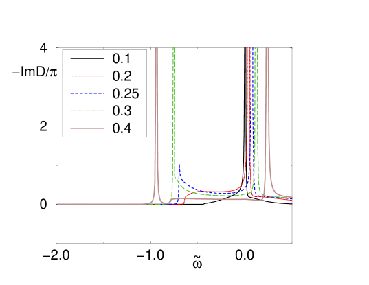
FIG. 1.: Absorption spectrum for $g_{ac}/g_{aa}=20$, $(n_{0}a^{3})^{1/2}=0.01$, for reduced temperatures $t$ shown in the legend.

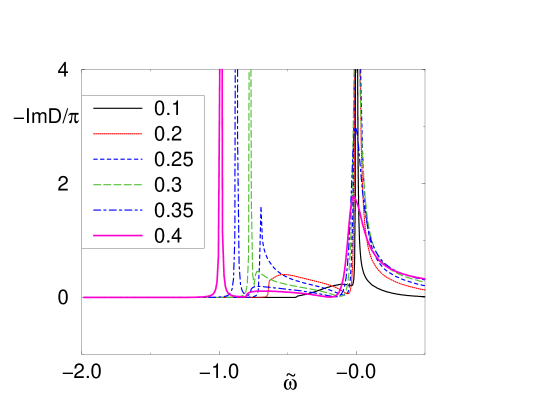
FIG. 2.: Absorption spectrum for $g_{ac}/g_{aa}=-20$, $(n_{0}a^{3})^{1/2}=0.01$, for reduced temperatures $t$ shown in the legend.

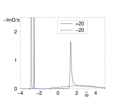
FIG. 3.: Absorption spectrum for $g_{ac}/g_{aa}=\pm 20$, $t=1.0$, for $(n_{0}a^{3})^{1/2}=0.01$.

REFERENCES

- [1] N. N. Bogoliubov, J. Phys. (USSR), 11, 23 (1947); for modern presentation, see A. L. Fetter and J. D. Walecka, Quantum Theory of Many-Particle Systems, McGraw Hill, (1995), Ch 10.
- [2] D. G. Fried, T. C. Killian, L. Willmann, D. Landhuis, S. C. Moss, D. Kleppner and T. J. Greytak, Phys. Rev. Lett. 81, 3811 (1998)
- [3] M. Ö. Oktel and L. S. Levitov, Phys. Rev. Lett. 83, 6 (1999)
- [4] C. J. Pethick and H. T. C. Stoof, xxx.lanl.gov/cond-mat/0102105
- [5] K. Johnsen and G. M. Kavoulakis, Phys. Rev. Lett. 86, 858 (2001)
- [6] V. N. Popov, Functional Integrals and Collective Modes, Cambridge University Press, New York, (1987); see also A. Griffin, Phys. Rev. B 53, 9341 (1996)