Dynamics of a two-mode Bose-Einstein condensate beyond mean field theory

Abstract

We study the dynamics of a two-mode Bose-Einstein condensate in the vicinity of a mean-field dynamical instability. Convergence to mean-field theory (MFT), with increasing total number of particles $N$, is shown to be logarithmically slow. Using a density matrix formalism rather than the conventional wavefunction methods, we derive an improved set of equations of motion for the mean-field plus the fluctuations, which goes beyond MFT and provides accurate predictions for the leading quantum corrections and the quantum break time. We show that the leading quantum corrections appear as decoherence of the reduced single-particle quantum state; we also compare this phenomenon to the effects of thermal noise. Using the rapid dephasing near an instability, we propose a method for the direct measurement of scattering lengths.

I Introduction

The effective low-energy Hamiltonian for $N$ interacting bosons confined in an external potential $V_{ext}$, is given in second-quantized form as

$$\hat{H}=\int\!d^{3}r{\bf\,}{\hat{\psi}}^{\dagger}\left[-\frac{\hbar^{2}}{2m}\nabla^{2}+V({\bf r})+\frac{g}{2}{\hat{\psi}}^{\dagger}{\hat{\psi}}\right]{\hat{\psi}}$$ (1)

where $V({\bf r})$ is the external trapping potential, and $m$ is the particle mass, $g$ is a coupling constant proportional to the s-wave scattering length, and ${\hat{\psi}},\hat{\psi}^{\dagger}$ are bosonic annihilation and destruction operator fields obeying the canonical commutation relation $\left[{\hat{\psi}}({\bf r}),{\hat{\psi}}^{\dagger}({\bf r}^{\prime})\right]=\delta({\bf r}-{\bf r}^{\prime})$. (This Hamiltonian is an effective low-energy approximation, in the sense that short wavelength degrees of freedom have been eliminated: it is applicable in the regime of ultracold scattering, where short distance modes are only populated virtually, during brief two-body collisions.)  At very low temperatures, Bose-Einstein condensation occurs, so that a large fraction of the particles occupy the same single-particle state, characterized by the single particle wave function $\Psi({\bf r},t).$  In this regime one can formulate a perturbative expansion in the small quantity $N^{-1/2}$, where $N$ is the number of particles in the condensate, whose result at leading order is the Gross-Pitaevskii nonlinear Schrödinger equation (GPE) governing the condensate wave function:

$$i\hbar\frac{\partial}{\partial t}\Psi({\bf r},t)=\left(-\frac{\hbar^{2}\nabla^{2}}{2m}+V_{ext}({\bf r})+g|\Psi({\bf r},t)|^{2}\right)\Psi({\bf r},t)\;,$$ (2)

The Gross-Pitaevskii mean field theory (MFT) provides a classical field equation for nonlinear matter waves, which is generally considered as ‘the classical limit’ of the Heisenberg equation of motion for the field operator ${\hat{\psi}}$ (which is of precisely the same form).  We can make precise the sense in which it is a classical limit, by reformulating the system governed by (8) in the path integral representation.  We will not actually use this formulation in this paper; we merely note the GPE is the saddlepoint equation that appears in a steepest descents approximation to the path integral.  This is precisely the standard semi-classical approximation, with the exception that $1/N$ is playing the role usually played by $\hbar$.  Hence despite the resemblance of the GPE to a Schrödinger equation, complete with finite $\hbar$, we can indeed identify MFT as the classical limit, in essentially the same sense as in the case $\hbar\rightarrow 0$, of the quantum field theory.  Because $N$ in current trapped dilute alkali gas BEC experiments is characteristically large (typically of the order $10^{5}-10^{8}$ atoms), qualitatively significant quantum corrections to MFT are hard to observe, and the GP theory is highly successful in predicting experimental results.

The entire field of quantum chaos is founded upon one property of the classical limit, however, which is that convergence to classicality as $\hbar\rightarrow 0$ is logarithmically slow if classical trajectories diverge exponentially.  This implies that we must expect strong quantum corrections to MFT in the vicinity of a dynamically unstable fixed point.  In particular, the quantum evolution will depart significantly from the classical approximation after a logarithmic ‘quantum break time’, which will be $\char 126\relax\log N$ in our case, as it is $\char 126\relax\log(1/\hbar)$ in the standard case .   In our case, the nature of this departure is that after the quantum break time, a condensate will become significantly depleted, as exponential production of quasi-particles transfers particles to orthogonal modes [1].  Depletion of the condensate means, by definition, that the single particle reduced density matrix (SPDM) becomes quantum mechanically less pure.  Hence for a condensate, just as the classical limit of the quantum field theory resembles the quantum mechanics of a single particle, so quantum corrections at the field theory level appear as quantum decoherence in the single-particle picture.  Since decoherence is most often considered as enforcing classicality, there is something like irony in this situation.  And it suggests that studying the corrections to MFT for Bose-Einstein condensates may give us some new insights into decoherence; and that some aspects of decoherence may be useful in understanding condensates beyond MFT.   This is the motivation for the work we now report.

In this paper we provide the details of a previously published study [2] of the correspondence between mean-field and exact quantum dynamics of a two-mode BEC. The model system contains an isolated dynamical instability for certain regions of parameter space. We show that quantum corrections in the vicinity of this unstable state, do indeed become significant on a short $\log(N)$ time scale, whereas quantum effects in other regions of phase space remain small $1/\sqrt{N}$ corrections. We present a simple theory that goes beyond MFT and provides accurate predictions of the leading quantum corrections, by taking one further step in the so called Bogoliubov-Born-Green-Kirkwood-Yvon (BBGKY) hierarchy. In accordance with our view of quantum corrections as decoherence, we use a density-matrix Bloch picture to depict the dephasing process. The density-matrix formalism has the additional advantage of allowing for initial conditions that are not covered by the Hartree-Fock-Bogoliubov Gaussian ansatz, and which better correspond to the physical state of the system.

FIG. 1.: Two-mode Bose-Einstein condensates: (a) a condensate in a double-well potential (b) a spinor condensate.

In section II we briefly review the model system and its experimental realizations. In section III we derive the mean-field equations of motion in the Bloch representation, and illustrate the main features of the produced dynamics for various parameter sets. Quantum corrections to the two-mode MFT are studied section IV, as well as an improved theory that predicts the leading corrections. In section V we consider the effect of thermal noise, and show an analogy between the quantum dephasing of the reduced single particle density operator and thermal decoherence. In section VI we present a potential application of the rapid decoherence near the dynamical instability of the two mode model, for the measurement of s-wave scattering-lengths. Discussion and conclusions are presented in section VII.

II The two-mode condensate

We consider a BEC in which particles can only effectively populate either one of two second-quantized modes. Two possible experimental realizations of this model are illustrated in Fig. 1. The first (Fig 1a) is a condensate confined in a double-well trap [3, 4, 5, 6, 7, 8] which may be formed by splitting a harmonic trap with a far off resonance intense laser sheet [9]. In this case single-particle tunneling provides a linear coupling between the local mode solutions of the individual wells, which can in principle be tuned over a wide range of strengths by adjusting the laser sheet intensity. The two-mode regime is reached when the self-interaction energy $gn$ is small compared to the spacing between the trap modes $\hbar\omega_{trap}$:

$$gn=\frac{4\pi\hbar^{2}a}{m}\frac{N}{4\pi l^{3}}\ll\frac{\hbar^{2}}{ml^{2}}=\hbar\omega_{trap}~{},$$ (3)

where $l$ is the characteristic trap size. Thus the two-mode condition is,

$$l\gg N|a|~{}.$$ (4)

The two-mode condition (4) may be met by double-well traps with characteristic frequencies of the order of 100 Hz, containing several hundred particles. When constructed, larger traps will maintain the two-mode limit at higher $N$.

The second experimental realization of a two-mode BEC is the effectively two-component spinor condensate [10, 11] depicted in Fig. 1b. In this case the linear coupling between the modes is provided by a near resonant radiation field [12, 13]. If collisions do not change spin states, the nonlinear interactions between the particles depend on three scattering lengths $a_{ij}$. In realisations of spinor condensates it is easy to ensure $a_{11}=a_{22}$ by symmetry, in which case the nonlinear interaction term becomes $\hat{H}_{int}=\int\!d^{3}r\,\hat{\cal H}_{int}({\bf r})$ for

$$\hat{\cal H}_{int} \propto\sum_{i,j}a_{ij}\hat{\psi}_{i}^{\dagger}\hat{\psi}_{i}\hat{\psi}_{j}^{\dagger}\hat{\psi}_{j}\to {a_{11}+a_{12}\over 2}(\hat{\psi}_{1}^{\dagger}\hat{\psi}_{1}+\hat{\psi}_{2}^{\dagger}\hat{\psi}_{2})^{2}$$ (6)

$$+{a_{11}-a_{12}\over 2}(\hat{\psi}_{1}^{\dagger}\hat{\psi}_{1}-\hat{\psi}_{2}^{\dagger}\hat{\psi}_{2})^{2}\;.$$

We can therefore define two healing lengths $\xi_{\pm}=1/\sqrt{\rho(a_{11}\pm a_{12})}$, where $\rho$ is the total density, characterizing the effect on the spatial state of the condensate of the two nonlinear terms. The two-mode regime, in which the spatial state is fixed and essentially independent of the internal state, is reached when $\xi_{-}$ becomes larger than the sample size (its largest dimension). Since for available alkali gases all $a_{ij}$ differ only by a few percent, $\xi_{-}<<\xi_{+}$, and hence the two-mode regime can be reached with $N<10^{4}$ atoms in weak, nearly spherical traps ($\omega_{trap}\leq 100$ Hz). Less isotropic traps obviously reach the two-mode regime only at smaller $N$. To extend the internal state two mode regime to larger $N$ we must make the trap weaker; for fixed $N$, $\xi_{-}$ scales with sample size $L$ as $L^{3/2}$. Hence to ensure $L/\xi_{-}<1$ for fixed $N$ requires a sufficiently large (weak) trap. For Rb and Na experiments, whose lifetimes are limited by three-body collisions, the slowing down of the two-mode dynamics at reduced total density should be more than compensated for by the extended condensate lifespan.

In both realizations, the many-body Hamiltonian reduces in the two-mode limit (and in the spinor realization also in the rotating-wave approximation) to the form,

$\displaystyle\hat{H}(t)=\frac{E_{1}+E_{2}}{2}({\hat{a}}_{1}^{\dagger}{\hat{a}}_{1}+{\hat{a}}_{2}^{\dagger}{\hat{a}}_{2})-\frac{\hbar\Omega}{2}\left({\hat{a}}_{1}^{\dagger}{\hat{a}}_{2}+{\hat{a}}_{2}^{\dagger}{\hat{a}}_{1}\right)$

$$+\hbar g\left[({\hat{a}}_{1}^{\dagger})^{2}{\hat{a}}_{1}^{2}+({\hat{a}}_{2}^{\dagger})^{2}{\hat{a}}_{2}^{2}\right]$$ (7)

where $E_{1}$ and $E_{2}$ are the two condensate mode energies, $\Omega$ is the coupling strength between the modes, $g$ is the two-body interaction strength, and ${\hat{a}}_{1},{\hat{a}}_{1}^{\dagger},{\hat{a}}_{2},{\hat{a}}_{2}^{\dagger}$ are particle annihilation and creation operators for the two modes. The total number operator $\hat{N}\equiv{\hat{a}}_{1}^{\dagger}{\hat{a}}_{1}+{\hat{a}}_{2}^{\dagger}{\hat{a}}_{2}$ commuted with $\hat{H}$ and may be replaced with the c-number $N$. Writing the self-interaction operators as $({\hat{a}}_{1}^{\dagger})^{2}{\hat{a}}_{1}^{2}+({\hat{a}}_{2}^{\dagger})^{2}{\hat{a}}_{2}^{2}=[\hat{N}^{2}+({\hat{a}}_{1}^{\dagger}{\hat{a}}_{1}-{\hat{a}}_{2}^{\dagger}{\hat{a}}_{2})^{2}]/2$ and discarding c-number terms, we obtain the two-mode Hamiltonian

$$\hat{H}=-\frac{\hbar\Omega}{2}\left({\hat{a}}_{1}^{\dagger}{\hat{a}}_{2}+{\hat{a}}_{2}^{\dagger}{\hat{a}}_{1}\right)+\frac{\hbar g}{2}\left({\hat{a}}_{1}^{\dagger}{\hat{a}}_{1}-{\hat{a}}_{2}^{\dagger}{\hat{a}}_{2}\right)^{2}~{}.$$ (8)

We will take $g$ and $\omega$ to be positive, since the relative phase between the two modes may be re-defined arbitrarily, and since without dissipation the overall sign of $\hat{H}$ is insignificant.

III Two-mode mean-field theory in the Bloch representation

The conventional wavefunction formalisms consider the evolution of ${\hat{a}}_{j}$ and its expectation value in a symmetry-breaking ansatz (where the symmetry being broken is that associated with conservation of $N$). Instead, we will examine the evolution of the directly observable quantities $\hat{a}_{i}^{\dagger}\hat{a}_{j}$, whose expectation values define the reduced single particle density matrix (SPDM) $R_{ij}\equiv\langle\hat{a}_{i}^{\dagger}\hat{a}_{j}\rangle/N$. Writing the Hamiltonian of Eq. (8) in terms of the SU(2) generators,

$${\hat{L}}_{x} \equiv \frac{{\hat{a}}_{1}^{\dagger}{\hat{a}}_{2}+{\hat{a}}_{2}^{\dagger}{\hat{a}}_{1}}{2}~{},$$ (9)

$${\hat{L}}_{y} \equiv \frac{{\hat{a}}_{1}^{\dagger}{\hat{a}}_{2}-{\hat{a}}_{2}^{\dagger}{\hat{a}}_{1}}{2i}~{},$$ (10)

$${\hat{L}}_{z} = \frac{{\hat{a}}_{1}^{\dagger}{\hat{a}}_{1}-{\hat{a}}_{2}^{\dagger}{\hat{a}}_{2}}{2}~{},$$ (11)

we obtain

$$\hat{H}=-\hbar\Omega{\hat{L}}_{x}+\frac{\hbar g}{2}{\hat{L}}_{z}^{2}\;.$$ (12)

The Heisenberg equations of motion for the three angular momentum operators of Eq. (9) read

$$\frac{d}{dt}{\hat{L}}_{x}=-\frac{i}{\hbar}[{\hat{L}}_{x},H] = -\frac{g}{2}({\hat{L}}_{y}{\hat{L}}_{z}+{\hat{L}}_{z}{\hat{L}}_{y})~{},$$ (13)

$$\frac{d}{dt}{\hat{L}}_{y}=-\frac{i}{\hbar}[{\hat{L}}_{y},H] = +\Omega{\hat{L}}_{z}+\frac{g}{2}({\hat{L}}_{x}{\hat{L}}_{z}+{\hat{L}}_{z}{\hat{L}}_{x})~{},$$ (14)

$$\frac{d}{dt}{\hat{L}}_{z}=-\frac{i}{\hbar}[{\hat{L}}_{z},H] = -\Omega{\hat{L}}_{y}~{}.$$ (15)

Thus the expectation values of the first-order operators ${\hat{L}}_{i}$ depend not only on themselves, but also on the second-order moments $\langle{\hat{L}}_{i}{\hat{L}}_{j}\rangle$. Similarly, the time evolution of the second-order moments depends on third-order moments; and so on. Consequently, we obtain the BBGKY hierarchy of equations of motion for the expectation-values,

$$\frac{d}{dt}\langle{\hat{L}}_{i}\rangle = f\left(\langle{\hat{L}}_{i^{\prime}}\rangle,\langle{\hat{L}}_{i^{\prime}}{\hat{L}}_{j^{\prime}}\rangle\right)~{},$$ (16)

$$\frac{d}{dt}\langle{\hat{L}}_{i}{\hat{L}}_{j}\rangle = f\left(\langle{\hat{L}}_{i^{\prime}}{\hat{L}}_{j^{\prime}}\rangle,\langle{\hat{L}}_{i^{\prime}}{\hat{L}}_{j^{\prime}}{\hat{L}}_{k^{\prime}}\rangle\right)~{},$$ (17)

$$\frac{d}{dt}\langle{\hat{L}}_{i}{\hat{L}}_{j}{\hat{L}}_{k}\rangle = f\left(\langle{\hat{L}}_{i^{\prime}}{\hat{L}}_{j^{\prime}}{\hat{L}}_{k^{\prime}}\rangle,\langle{\hat{L}}_{i^{\prime}}{\hat{L}}_{j^{\prime}}{\hat{L}}_{k^{\prime}}{\hat{L}}_{l^{\prime}}\rangle\right)~{},$$ (18)

$$\vdots$$ (19)

where $i,j,k,\dots,i^{\prime},j^{\prime},k^{\prime},l^{\prime},\dots=x,y,z$. In order to obtain a closed set of equations of motion, the hierarchy of Eq. (16) must be truncated at some stage by approximating the $N$-th order expectation value in terms of all lower-order moments.

The lowest-order truncation of Eq. (16) is obtained by approximating the second-order expectation values $\langle{\hat{L}}_{i}{\hat{L}}_{j}\rangle$ as products of the first-order moments $\langle{\hat{L}}_{i}\rangle$ and $\langle{\hat{L}}_{j}\rangle$:

$$\langle{\hat{L}}_{i}{\hat{L}}_{j}\rangle\approx\langle{\hat{L}}_{i}\rangle\langle{\hat{L}}_{j}\rangle~{}.$$ (20)

The equations of motion for the single-particle Bloch vector

$${\bf{\vec{s}}}=(s_{x},s_{y},s_{z})\equiv\left(\frac{2\langle{\hat{L}}_{x}\rangle}{N},\frac{2\langle{\hat{L}}_{y}\rangle}{N},\frac{2\langle{\hat{L}}_{z}\rangle}{N}\right),$$ (21)

Then read

$${\dot{s}}_{x} = -\kappa s_{z}s_{y}~{},$$ (22)

$${\dot{s}}_{y} = \Omega s_{z}+\kappa s_{z}s_{x}~{},$$ (23)

$${\dot{s}}_{z} = -\Omega s_{y}~{},$$ (24)

where $\kappa=gN/2$. Equations (22) describe rotations of the Bloch vector ${\bf{\vec{s}}}$, and so the norm $|{\bf{\vec{s}}}|$ is conserved in MFT. Consequently, for a pure SPDM, Eq. (22) are completely equivalent to the two-mode Gross-Pitaevskii equation [6],

$$i\frac{\partial}{\partial t}a_{1} = \kappa a_{1}-\Omega a_{2}$$ (26)

$$i\frac{\partial}{\partial t}a_{2} = \kappa a_{2}-\Omega a_{1}$$ (27)

where $a_{1}$ and $a_{2}$ are the c-number coefficients replacing the creation and annihilation operators of Eq. (9)

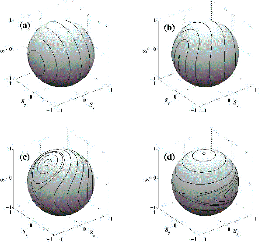
FIG. 2.: Mean-field trajectories at (a)$\kappa=0$, (b)$\kappa=1.02\Omega$, (c)$\kappa=2\Omega$, and (d)$\kappa=20\Omega$.

In Fig. 2 we plot mean-field trajectories at four different $\kappa/\Omega$ ratios. The nonlinear Bloch equations (22) depict a competition between linear Rabi oscillations in the $s_{y}s_{z}$-plane and nonlinear oscillations in the $s_{x}s_{y}$-plane. For a noninteracting condensate (Fig. 2a) the trajectories on the Bloch sphere depict harmonic Rabi oscillations about the $s_{x}$ axis. As $\kappa$ increases the oscillations become increasingly anharmonic. As long as $\kappa<\Omega$ the nonlinearities may be treated as perturbation. However, above the critical value $\kappa=\omega$ (Fig. 2b), there are certain regions in phase-space which are dominated by the nonlinear term. The stationary point ${\bf{\vec{s}}}=(-1,0,0)$, corresponding to the Josephson $\pi$-state (equal populations and a $\pi$ phase-difference), becomes dynamically unstable and the two trajectories passing asymptotically close to it form a “figure-eight”. The region outside these limiting trajectories is dominated by the linear oscillations whereas inside the nonlinear term prevails. Starting at the critical value of $\kappa=2\Omega$ (Fig. 2c) population prepared in one of the modes remains trapped in the half-sphere it originated from, conducting oscillations with a non-vanishing time averaged population imbalance $\langle s_{z}\rangle_{t}\neq 0$. This phenomenon was termed “macroscopic self-trapping” [6]. Finally, when $\kappa\gg\Omega$ (Fig. 2d) the nonlinearity dominates the entire Bloch sphere, except for a narrow band about the $s_{z}=0$ plain.

IV Quantum corrections and Bogoliubov backreaction

In the vicinity of the dynamically unstable point, we expect MFT to break down on a time scale only logarithmic in $N$. In order to verify this prediction, we solve the full $N$-body problem exactly, by fixing the total number of particles $N$, thereby restricting the available phase-space to Fock states of the type $|\,{n,N-n}\,\rangle$ with $n$ particles in one mode and $N-n$ particles in the other mode, $n$ ranging from 0 to $N$. Thus we obtain an $N+1$ dimensional representation for the Hamiltonian (12) and the $N$-body density operator $\hat{\rho}$:

$$H_{m,n} = \langle\,{m,N-m}\,|\,\hat{H}\,|\,{n,N-n}\,\rangle~{},$$ (28)

$$\rho_{m,n} = \langle\,{m,N-m}\,|\,\hat{\rho}\,|\,{n,N-n}\,\rangle~{},$$ (29)

for $m,n=0,1,\dots,N$. The exact quantum solution is obtained numerically by propagating $\hat{\rho}$ according to the Liouville von-Neumann equation

$$i\hbar\dot{\hat{\rho}}=[\hat{H},\hat{\rho}]~{}.$$ (30)

Using the Hamiltonian of Eq. (12) to evaluate the matrix elements of Eq. (28) and substituting into Eq. (30), we obtain dynamical equations for the N-body density matrix:

$$i\hbar\dot{\rho}_{m,n} = -\frac{\Omega}{2}\left[\sqrt{m(N-m+1)}\rho_{m-1,n}\right.$$ (31)

$$+\sqrt{(m+1)(N-m)}\rho_{m+1,n}$$ (32)

$$-\sqrt{n(N-n+1)}\rho_{m,n-1}$$ (33)

$$\left.-\sqrt{(n+1)(N-n)}\rho_{m,n+1}\right]$$ (34)

$$+\frac{g}{4}\left[m^{2}-(N-m)^{2}-n^{2}+(N-n)^{2}\right]\rho_{m,n}~{}.$$ (35)

Equations (31) are solved numerically, using a Runge-Kutta algorithm. In fig. 3 we plot exact quantum trajectories starting with all particles in one mode, for increasingly large $N$ ($\kappa$ being fixed) versus the corresponding mean-field trajectory. While MFT assumes a persistently pure single particle state, quantum corrections to MFT appear in the single-particle picture, as decoherence of the SPDM. When the mean-field trajectory stays away from the instability (Fig. 3a) the quantum trajectories indeed enter the interior of the unit Bloch sphere at a rate that vanishes as $1/\sqrt{N}$. However, when the mean-field trajectory includes the unstable state (Fig. 3b), we observe a sharp break of the quantum dynamics from the mean-field trajectory at a time that only grows slowly with $N$.

In accordance with our picture of quantum corrections as decoherence, and in order to obtain a more quantitative view of the entanglement-induced dephasing process, we plot the von Neumann entropy

$$S=Tr(R\ln R)=-\frac{1}{2}\ln\left[\frac{(1+|{\bf{\vec{s}}}|)^{(1+|{\bf{\vec{s}}}|)}(1-|{\bf{\vec{s}}}|)^{(1-|{\bf{\vec{s}}}|)}}{4}\right]$$ (36)

of the exact reduced single-particle density operator, as a function of the rescaled time $\Omega t$ for the same initial conditions as in Fig. 3. The results are shown in Fig. 4. Since the entropy of mean-field trajectories is identically zero, $S$ may serve as a measure of the deviation from MFT. When the mean-field trajectory is stable (Fig. 4a), the single particle entropy grows at a steady rate which vanishes as $N$ is increased. The variations in the entropy growth curve are a function of the distance from the instability. Near the instability (Fig. 4b) quantum corrections grow rapidly at a rate which is independent of $N,$ and the time at which this divergence takes place (the quantum break time) evidently grows only as $\log(N)$.

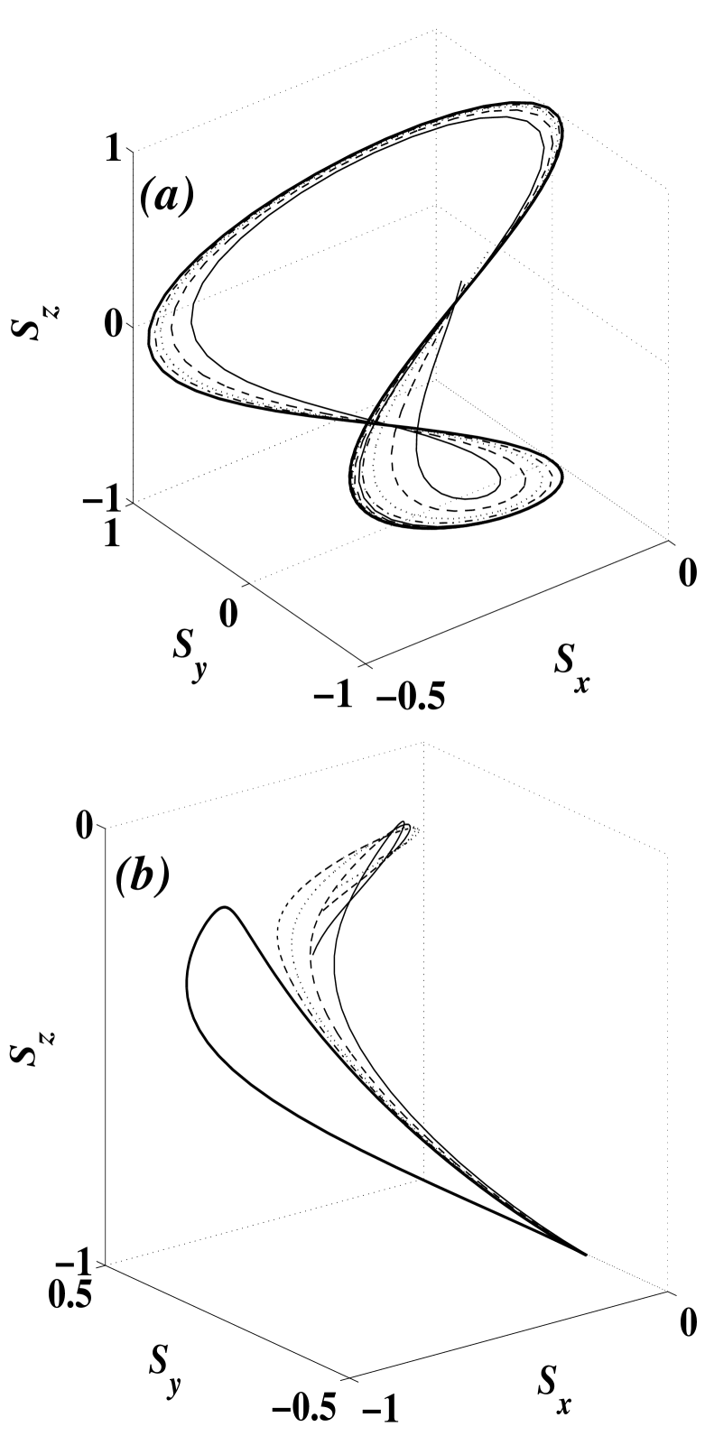
FIG. 3.: Exact quantum trajectories starting with all particles in one mode, with $N=50$ (—–), 100 ($---$), 200 ($\cdots$) and 400 ($-\cdot-$) particles vs. the corresponding mean-field trajectory (—–) for (a) $\kappa=\Omega$ and (b) $\kappa=2\Omega$.

Since MFT can thus easily fail near dynamical instabilities, it is highly desirable to obtain an improved theory in which Bloch-space trajectories would be allowed to penetrate into the unit sphere without having to simulate the entire $N$-body dynamics. In fact, such an improved non-unitary theory is easily derived using the next level of the BBGKY hierarchy (16). This hierarchy truncation approach is in fact a systematic perturbative approximation; but it is state-dependent. That is, it provides a perturbative approximation, not to the general evolution, but to the evolution of a special class of initial states, within which the perturbative parameter is small. In the case of ultracold bosons, the phenomenon of Bose-Einstein condensation ensures that there is a commonly realisable class of states in which the system is a mildly fragmented condensate. In our two mode model, this means that the two eigenvalues of $R$ are $f$ and 1-$f$ for $f\ll 1$; and so from such initial states we can approximate the evolution perturbatively using $f$ as our small parameter.

FIG. 4.: Growth of the von Neumann entropy $S$ of the quantum reduced single-particle density operator, at (a) $\kappa=\Omega$ and (b) $\kappa=2\Omega$, for N=10 ($-\cdot-$), 20 ($\cdot\cdot\cdot$), 40 ($---$), 80 (——), 160 (- . - . -), and 320 (- - - -) particles. Initial conditions are the same as in Fig. 3.

To zeroth order in $f$, $R$ is by definition a pure state, and hence we have the MFT evolution on the surface of the Bloch sphere. Going to next order in $f$ can be achieved by truncating the BBGKY hierarchy at one order higher. We take ${\hat{L}}_{i}=L_{i}+\hat{\delta L_{i}}$, where the c-number $L_{i}$ is ${\cal O}(N)$ and all the matrix elements of $\hat{\delta L_{i}}$ remain smaller than ${\cal O}(N\sqrt{f})$ throughout the evolution of the system. The second order moments,

$$\Delta_{ij}=4N^{-2}\left(\langle{\hat{L}}_{i}{\hat{L}}_{j}+{\hat{L}}_{j}{\hat{L}}_{i}\rangle-2\langle{\hat{L}}_{i}\rangle\langle{\hat{L}}_{j}\rangle\right)~{},$$ (37)

will then be of order $f$. Writing the Heisenberg equations of motion for the first- and second-order operators ${\hat{L}}_{i},{\hat{L}}_{i}{\hat{L}}_{j}$, taking their expectation values and truncating Eq. (16) by approximating

$\displaystyle\langle{\hat{L}}_{i}{\hat{L}}_{j}{\hat{L}}_{k}\rangle\approx\langle{\hat{L}}_{i}{\hat{L}}_{j}\rangle\langle{\hat{L}}_{k}\rangle+\langle{\hat{L}}_{i}\rangle\langle{\hat{L}}_{j}{\hat{L}}_{k}\rangle+\langle{\hat{L}}_{i}{\hat{L}}_{k}\rangle\langle{\hat{L}}_{j}\rangle$

$$-2\langle{\hat{L}}_{i}\rangle\langle{\hat{L}}_{j}\rangle\langle{\hat{L}}_{k}\rangle\;.$$ (38)

instead of the mean-field approximation (20), we obtain the following set of nine equations for the first- and second-order moments:

$${\dot{s}}_{x} = -\kappa s_{z}s_{y}-\frac{\kappa}{2}\Delta_{yz}$$ (39)

$${\dot{s}}_{y} = \omega s_{z}+\kappa s_{z}s_{x}+\frac{\kappa}{2}\Delta_{xz}$$ (40)

$${\dot{s}}_{z} = -\omega s_{y}$$ (41)

$${\dot{\Delta}}_{xz} = -\omega\Delta_{xy}-\kappa s_{z}\Delta_{yz}-\kappa s_{y}\Delta_{zz}$$ (42)

$${\dot{\Delta}}_{yz} = \omega(\Delta_{zz}-\Delta_{yy})+\kappa s_{z}\Delta_{xz}+\kappa s_{x}\Delta_{zz}$$ (43)

$${\dot{\Delta}}_{xy} = (\omega+\kappa s_{x})\Delta_{xz}-\kappa s_{y}\Delta_{yz}+\kappa s_{z}(\Delta_{xx}-\Delta_{yy})$$ (44)

$${\dot{\Delta}}_{xx} = -2\kappa s_{y}\Delta_{xz}-2\kappa s_{z}\Delta_{xy}$$ (45)

$${\dot{\Delta}}_{yy} = 2(\omega+\kappa s_{x})\Delta_{yz}+2\kappa s_{z}\Delta_{xy}$$ (46)

$${\dot{\Delta}}_{zz} = -2\omega\Delta_{yz}~{}.$$ (47)

Equations (39) will be referred to as the “Bogoliubov backreaction equations” (BBR), because they demonstrate how the mean-field Bloch vector ${\bf{\vec{s}}}$ drives the fluctuations $\Delta_{ij}$ – which is the physics described by the Bogoliubov theory of linearized quantum corrections to MFT; but they also make the Bloch vector subject in turn to backreaction from the fluctuations, via the coupling terms $-\kappa\Delta_{yz}/2$ and $\kappa\Delta_{xz}/2$. This back-reaction has the effect of breaking the unitarity of the mean-field dynamics. Consequently, the BBR trajectories are no longer confined to the surface of the Bloch sphere, but penetrate to the interior (representing mixed-state $R_{ij}$, with two non-zero eigenvalues). (Obviously, if the trajectories penetrate the sphere too deeply, so that the smaller eigenvalue $f$ ceases to be small, the entire approach of perturbing in $f$ will break down.)

In order to demonstrate how the BBR equations (39) improve on MFT, we compare trajectories obtained by these two formalisms to the exact 50-particle trajectories of Fig. 3. Both the $\kappa=\Omega$ stable mean-field trajectory and the $\kappa=2\Omega$ unstable mean-field trajectory cases are plotted in Fig. 5a and Fig. 5b, respectively. The initial conditions for the BBR equations are determined by the initial state $|\,{N,0}\,\rangle$ to be

$$s_{z} = -1,$$ (48)

$$\Delta_{xx} = \Delta_{yy}=2/N,$$ (49)

$$s_{x} = s_{y}=\Delta_{xy}=\Delta_{xz}=\Delta_{yz}=\Delta_{zz}=0~{}.$$ (50)

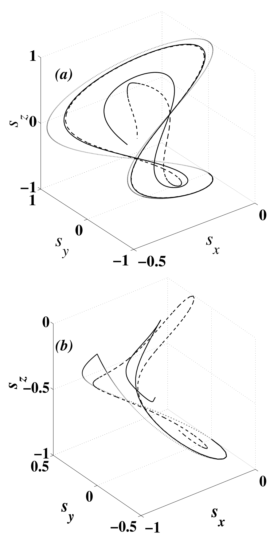
FIG. 5.: Mean field ($\cdot\cdot\cdot$), Bogoliubov back-reaction ($---$) and exact 50 particles (—–) trajectories starting with all particles in one mode, at (a) $\kappa=\Omega$ and (b) $\kappa=2\Omega$.

The approximation of Eq. (38) ignores terms smaller than ${\cal{O}}(f^{3/2})$. It is therefore better than the mean-field approximation (20) by a factor of $f^{1/2}$. Consequently, as is clearly evident from Fig. 5a, the BBR equations (39) are far more successful than the mean-field equations (22) in tracing the full quantum dynamics. However, for any realistic number of particles, the improvement is hardly necessary, as MFT would be accurate for very long times. On the other hand, when the mean-field trajectory approaches the instability (Fig. 5b), the BBR theory provides an accurate prediction of the leading quantum corrections. Of course, since the BBR equations account for only six moments unobserved by MFT, the period of the still quasiperiodic BBR motion is shorter than that of the exact evolution and the BBR trajectory eventually deviates from the quantum trajectory. Nevertheless, the BBR formalism provides a simple and efficient method to predict the quantum break time in large ($>1000$ particles) condensates, for which full $N$-body simulations are restricted by available computation power.

The BBR equations (39) are in fact identical to the equations of motion one would obtain, for the same quantities, using the Hartree-Fock-Bogoliubov Gaussian ansatz, in which second-order moments $\Delta_{ij}$ are initially factorized as $\Delta_{ij}=\delta_{i}\delta_{j}$ ($i,j=x,y,z$). Using this ansatz, the factorization persists and the time evolution of $\delta_{x},\delta_{y}$, and $\delta_{z}$ is equivalent to that of perturbations of the mean-field equations (22):

$${\dot{\delta}}_{x} = -\kappa(s_{z}\delta_{y}+s_{y}\delta_{z})~{},$$ (51)

$${\dot{\delta}}_{y} = \omega\delta_{z}+\kappa(s_{z}\delta_{x}+s_{x}\delta_{z})~{},$$ (52)

$${\dot{\delta}}_{z} = -\omega\delta_{y}~{}.$$ (53)

Thus our equations for $\Delta_{ij}$ are in a sense equivalent to the usual Bogoliubov equations. The quantitative advantage of our approach therefore lies entirely in the wider range of initial conditions that it admits, which may more accurately represent the exact initial conditions. For instance, a Gaussian approximation will have $\Delta_{xx}={\cal O}(1)$ in the ground state, where in fact $\Delta_{xx}={\cal O}(N^{-1})$. This leads to an error of order $N^{-1/2}$ in the Josephson frequency computed by linearizing (39) around the ground state, even though the Gaussian backreaction result should naively be accurate at this order. Our SPDM approach does not have this flaw, which is presumably the two-mode version of the Hartree-Fock-Bogoliubov spectral gap [14].

V Dephasing due to thermal noise

Decoherence is generally considered as suppressing quantum effects [15]. Ironically, in our case the leading quantum corrections to the effectively classical MFT, are themselves decoherence of the single-particle state of the condensate. Therefore, it is interesting to study the effect of a realistic decoherence process, originating in the coupling to a bath of unobserved degrees of freedom, on the interparticle entanglement process, described in the previous section.

The main source of decoherence in BEC’s is the thermal cloud of particles surrounding the condensate. Thermal particles scattering off the condensate mean field will for example, cause phase diffusion [16] at a rate $\Gamma$ proportional to the thermal cloud temperature. For internal states not entangled with the condensate spatial state, $\Gamma$ may be as low as $10^{-5}$ Hz under the coldest experimental conditions, whereas for a double well the rate may reach $10^{-1}$ Hz. Further sources of decoherence may be described phenomenologically with a larger $\Gamma$.

We account effect of thermal noise on the two-mode dynamics by using the quantum kinetic master equation [5],

$$\dot{\rho}=\frac{i}{\hbar}[\rho,H]-\frac{\Gamma}{2}\sum_{j=1,2}\left[{\hat{a}}_{j}^{\dagger}{\hat{a}}_{j},\left[{\hat{a}}_{j}^{\dagger}{\hat{a}}_{j},\rho\right]\right]~{}.$$ (54)

Once again, we solve for ${\bf{\vec{s}}}(t)$ using either one of three methods:

(a) MFT - The decoherence term in Eq. (54) introduces an exact $T_{2}=1/\Gamma$ transversal relaxation term into the mean-field equations of motion:

$${\dot{s}}_{x} = -\kappa s_{z}s_{y}-\Gamma s_{x}~{},$$ (55)

$${\dot{s}}_{y} = \omega s_{z}+\kappa s_{z}s_{x}-\Gamma s_{y}~{},$$ (56)

$${\dot{s}}_{z} = -\omega s_{y}~{}.$$ (57)

(b) BBR - Evolving the first- and second-order operators according to Eq. (54), taking their expectation values and truncating the hierarchy at the next level, we obtain the modified BBR equations,

$${\dot{s}}_{x} = -\kappa s_{z}s_{y}-\frac{\kappa}{2}\Delta_{yz}-\Gamma s_{x},$$ (58)

$${\dot{s}}_{y} = \omega s_{z}+\kappa s_{z}s_{x}+\frac{\kappa}{2}\Delta_{xz}-\Gamma s_{y},$$ (59)

$${\dot{s}}_{z} = -\omega s_{y},$$ (60)

$${\dot{\Delta}}_{xz} = -\omega\Delta_{xy}-\kappa s_{z}\Delta_{yz}-\kappa s_{y}\Delta_{zz}-\Gamma\Delta_{xz},$$ (61)

$${\dot{\Delta}}_{yz} = \omega(\Delta_{zz}-\Delta_{yy})+\kappa s_{z}\Delta_{xz}+\kappa s_{x}\Delta_{zz}-\Gamma\Delta_{yz},$$ (62)

$${\dot{\Delta}}_{xy} = (\omega+\kappa s_{x})\Delta_{xz}$$ (63)

$$-\kappa s_{y}\Delta_{yz}+\kappa s_{z}(\Delta_{xx}-\Delta_{yy})-4\Gamma(\Delta_{xy}+s_{x}s_{y}),$$ (64)

$${\dot{\Delta}}_{xx} = -2\kappa s_{y}\Delta_{xz}-2\kappa s_{z}\Delta_{xy}-2\Gamma(\Delta_{xx}-\Delta_{yy}-2s_{y}^{2}),$$ (65)

$${\dot{\Delta}}_{yy} = 2(\omega+\kappa s_{x})\Delta_{yz},$$ (66)

$$+2\kappa s_{z}\Delta_{xy}-2\Gamma(\Delta_{yy}-\Delta_{xx}-2s_{x}^{2}),$$ (67)

$${\dot{\Delta}}_{zz} = -2\omega\Delta_{yz}~{},$$ (68)

(c) Exact quantum solution - obtained by numerically propagating the full $N$-particle density matrix under Eq. (54).

In Fig. 6 we compare the Von-Neumann entropy of the exact $N$-body density operator as a function of time for exponentially increasing $N$, to the mean-field entropy. Due to the thermal noise, mean-field trajectories are no longer confined to the zero-entropy sphere. However, whereas the quantum break time in the absence of thermal noise has grown as $\log(N)$ (see Fig. 4b), it is clear from Fig. 6 that in the presence of this dephasing mechanism it saturates to a finite value. Thus, while we may have naively expected decoherence to reduce quantum corrections and thereby improve MFT, in fact the addition of thermal dephasing has significantly damaged classical-quantum correspondence.

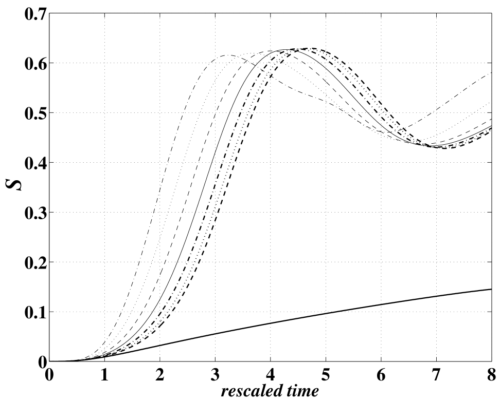
FIG. 6.: Growth of the von Neumann entropy $S$ of the quantum reduced single-particle density operator in the presence of thermal noise ( $\Gamma=10^{-2}\Omega$), at $\kappa=2\Omega$, for N=10 ($-\cdot-$), 20 ($\cdot\cdot\cdot$), 40 ($---$), 80 (——), 160 (- . - ), 320 (- - - -, and 640 (. . .) particles. Bold solid curve corresponds to the mean field entropy. Initial conditions are the same as in Fig. 3.

In Fig. 7, we summarize the results of numerous dynamical calculations conducted for various values of the particle number $N$ and of the thermal noise $\Gamma$, by plotting the time at which the entropy reaches a given value. The curves are obtained using the modified BBR equations (58) whereas the circles and squares depict exact quantum results (limited by computation power to $N\sim 10^{3}$ particles) for two limiting values of $\Gamma$. The BBR equations provide accurate predictions of the initial decoherence rate and the quantum break time even within this limited range of $N$ (and the agreement between the exact quantum results and the BBR predictions would become still better for higher numbers of particles). Once more, we observe the logarithmic growth of the quantum break time with $N$ in the zero temperature ($\Gamma=0$) limit. However, when the temperature is finite, there is a saturation of the quantum break time to values which are well below the mean-field thermal dephasing times, in agreement with Fig. 6.

Instead of observing the quantum break time as a function of the number of particles for a given degree of thermal noise, we can monitor the thermal decoherence time as a function of temperature, for any given number of particles. Viewing Fig. 7 this way, it is evident that in the mean-field limit ($1/\sqrt{N}\rightarrow 0$) the purely thermal dephasing time also grows only logarithmically with the temperature, Comparing this result to the $\log(N)$ growth of the quantum break time in the zero-temperature limit, we can see that thermal noise and quantum noise have essentially similar effects on the system.  And Figs. 6 and 7 together are in complete agreement with the prediction that the entropy of a dynamically unstable quantum system coupled to a reservoir[17], or of a stable system coupled to a dynamically unstable reservoir, will grow linearly with time, at a rate independent of the system-reservoir coupling, after an onset time proportional to the logarithm of the coupling [18, 19]. Thus, one can really consider the Bogoliubov fluctuations as a reservoir [20], coupled to the mean field with a strength proportional to $1/N$.  The $N\leftrightarrow 1/T$ analogy is even further extended by the saturation for any finite $N$, of the thermal dephasing time at low $T$, in the same way that the quantum break time for a finite $T$ saturates at high $N$.  Due to this quantum saturation, quantum corrections can be experimentally distinguished from ordinary thermal effects which do not saturate the dephasing rate at low temperature.

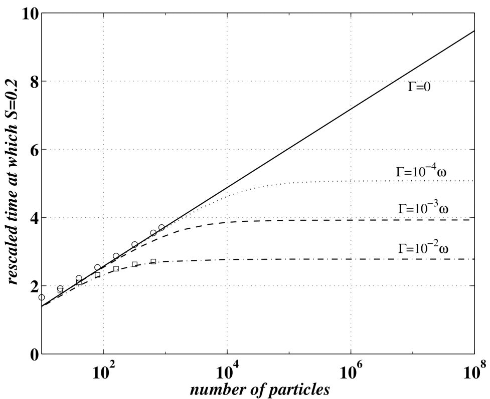
FIG. 7.: Time at which $S$ reaches 0.2 as a function of the particle number $N$, according to the BBR equations (39), modified to include thermal phase-diffusion. Four different values of $\Gamma$ are shown: $\Gamma=0$ (—–), $\Gamma=10^{-4}\Omega$ ($\cdot\cdot\cdot$), $\Gamma=10^{-3}\Omega$ ($---$), and $\Gamma=10^{-2}\Omega$ ($-\cdot-$). Exact quantum results are presented for $\Gamma=0$ (circles) and $\Gamma=10^{-2}\Omega$ (squares). Initial conditions, $\kappa$ and $\Omega$ are the same as in Fig. 6.

VI Scattering-length measurements

After indicating how condensate decoherence at dynamical instabilities can connect principles established in different areas of physics, we briefly note that it can also have practical applications.  Rapid decoherence in the vicinity of the unstable $\pi$-state of the two-mode condensate may serve for the direct measurement of scattering lengths. As demonstrated in Fig. 8, the mean-field trajectory of a condensate which is prepared initially in one of the modes, would only pass through the rapidly dephasing unstable point when $\kappa=2\Omega$. Thus, the self-interactions energy $\kappa$ can be determined by measuring the entropy at a fixed time as a function of the coupling frequency $\Omega$, resulting in a sharp line about $\Omega=\kappa/2$, as depicted in Fig. 9.

Experimentally, the single-particle entropy is measurable, in the internal state realization of our model, by applying a fast Rabi pulse and measuring the amplitude of the ensuing Rabi oscillations, which is proportional to the Bloch vector length $|{\bf{\vec{s}}}|$. (Successive measurements with Rabi rotations about different axes, i.e. by two resonant pulses differing by a phase of $\pi/2$, will control for the dependence on the angle of ${\bf{\vec{s}}}$). In a double well realization, one could determine the single-particle entropy by lowering the potential barrier, at a moment when the populations on each side were predicted to be equal, to let the two parts of the condensate interfere. The fringe visibility would then be proportional to $|{\bf{\vec{s}}}|$ [9].

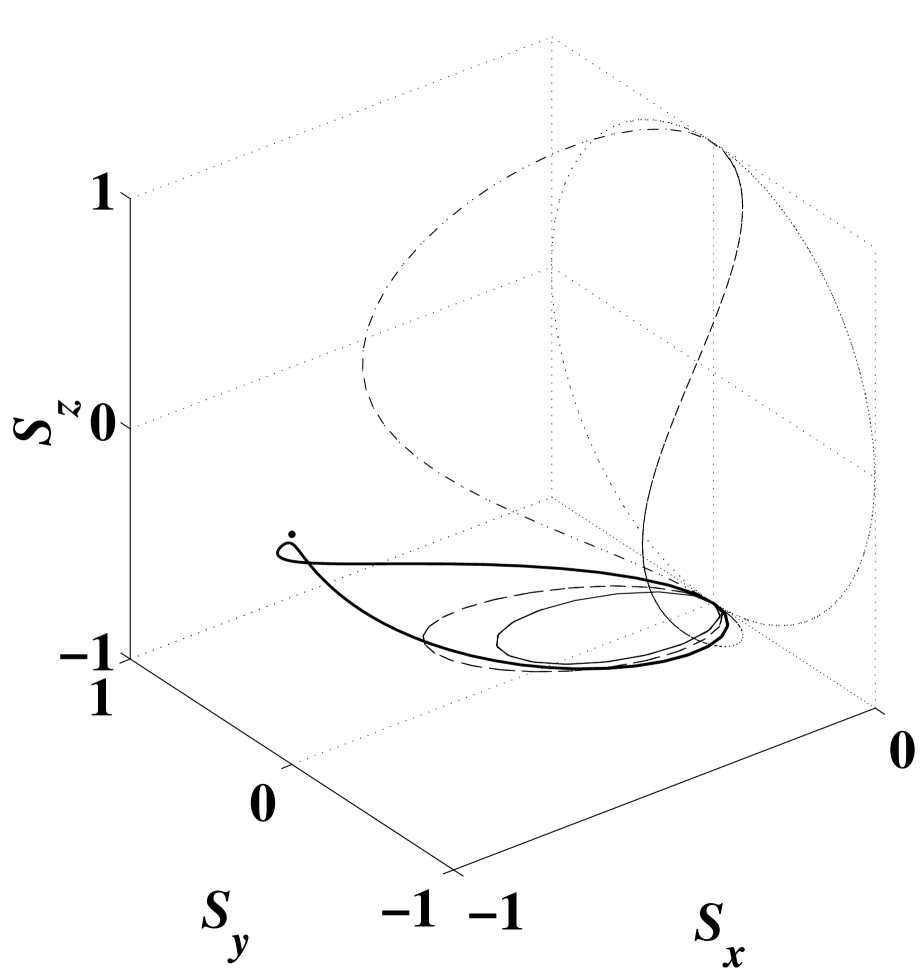
FIG. 8.: Mean-field trajectories starting at ${\bf{\vec{s}}}=(0,0,-1)$ for $\kappa=0$ ($\dots$), $\kappa=\Omega$ ($-\cdot-$), $\kappa=2\Omega$ (—–), $\kappa=3\Omega$ ($---$), and $\kappa=4\Omega$ (—–). The dot at ${\bf{\vec{s}}}=(-1,0,0)$ marks the dynamical instability.

VII Conclusions

To conclude, we have shown that significant quantum corrections to the Gross-Pitaevskii MFT, in the vicinity of its dynamical instabilities, can be measured in a two-mode BEC under currently achievable experimental conditions. We have derived a simple theory that accurately predicts the leading quantum corrections and the quantum break time.  By applying to condensate physics some insights from studies of decoherence, we have found evidence that MFT dynamical instabilities cause linear growth of the single-particle entropy at a rate independent of $N.$  And from condensate physics we have learned something about decoherence: we have identified a form of decoherence which degrades quantum-classical correspondence, instead of improving it.

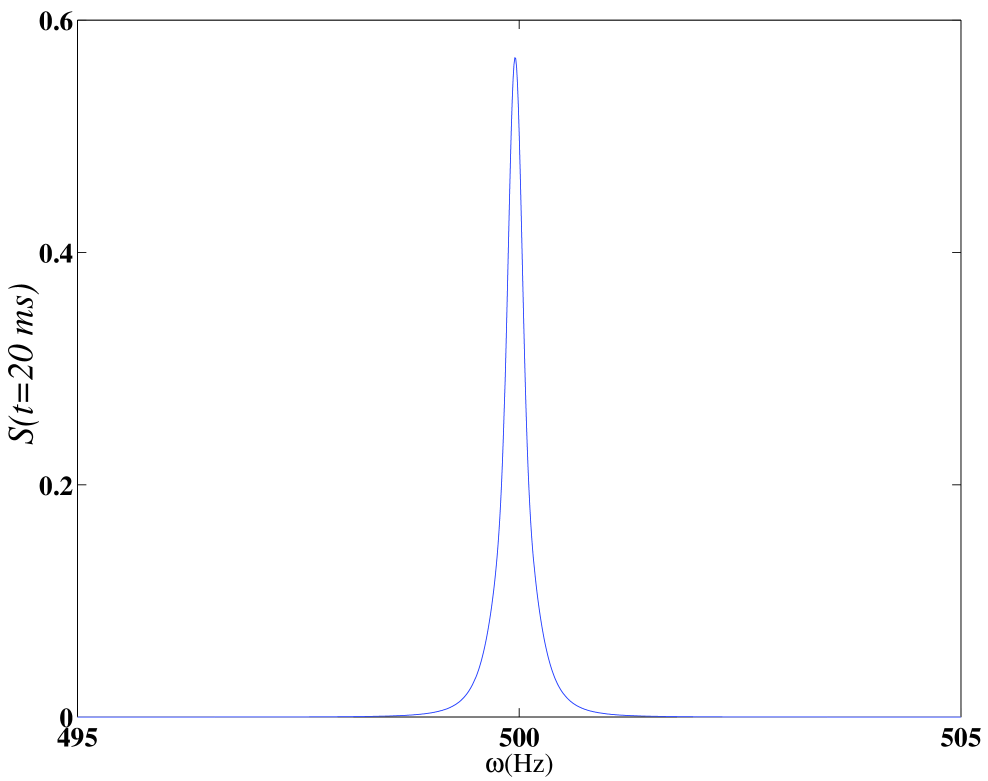
FIG. 9.: von Neumann entropy $S$ after 20 ms of propagation according to the BBR equations (58) with $\kappa=1$ KHz and $\Gamma=10^{-4}$ Hz, starting with the entire condensate of $N=10^{5}$ particles in one mode, as a function of the coupling frequency $\Omega$.

Our picture of quantum backreaction in BECs as decoherence suggests new lines of investigation for both experiment and theory: measurements of single-particle entropy in condensates, descriptions of condensates with mixed single particle states (instead of the usual macroscopic wave functions), and general questions of decoherence under nonlinear evolution. Exploring these possibilities, beyond the two-mode model considered here, provides many goals for further research.

REFERENCES

- [1] Y. Castin and R. Dum, Phys. Rev. Lett. 79, 3553 (1997).
- [2] A. Vardi and J. R. Anglin, Phys. Rev. Lett. , 86, 568 (2001).
- [3] J. Javanainen, Phys. Rev. Lett. 57, 3164 (1986); J. Javanainen and S. M. Yoo, Phys. Rev. Lett. 76, 161 (1996).
- [4] M. W. Jack, M. J. Collett, and D. F. Walls, Phys. Rev. A 54, R4625 (1996); G. J. Milburn, J. Corney, E. M. Wright, D. F. Walls, Phys. Rev. A 55, 4318 (1997); A. S. Parkins and D. F. Walls Phys. Rep. 303, 1 (1998).
- [5] J. Ruostekoski and D. F. Walls, Phys. Rev. A 58, R50 (1998).
- [6] A. Smerzi, S. Fantoni, S. Giovanazzi, and S. R. Shenoy, Phys. Rev. Lett. 79, 4950 (1997); S. Raghavan, A. Smerzi, S. Fantoni, and S. R. Shenoy, Phys. Rev. A 59, 620 (1999); I. Marino, S. Raghavan, S. Fantoni, S. R. Shenoy, and A. Smerzi, Phys. Rev. A 60, 487 (1999).
- [7] I. Zapata, F. Sols, and A. J. Leggett, Phys. Rev. A 57, R28 (1998).
- [8] P. Villain and M. Lewenstein, Phys. Rev. A 59, 2250 (1999).
- [9] M. R. Andrews, C. G. Townsend, H. J. Miesner, D. S. Durfee, D. M. Kurn, and W. Ketterle, Science 275, 637 (1997).
- [10] M. R. Matthews, B. P. Anderson, P. C. Haljan, D. S. Hall, M. J. Holland, J. E. Williams, C. E. Wieman, and E. A. Cornell, Phys. Rev. Lett. 83, 3358 (1999).
- [11] C. J. Myatt, E. A. Burt, R. W. Ghrist, E. A. Cornell, and C. E. Wieman, Phys. Rev. Lett. 78, 586 (1997).
- [12] M. R. Matthews, D. S. Hall, D. S. Jin, J. R. Ensher, C. E. Wieman, E. A. Cornell, F. Dalfovo, C. Minniti, and S. Stringari, Phys. Rev. Lett. 81, 243 (1998); J. Williams, R. Walser, J. Cooper, E. Cornell, and M. Holland, Phys. Rev. A 59, R31 (1999).
- [13] Patrik Öhberg and Stig Stenholm, Phys. Rev. A 59, 3890 (1999).
- [14] A. Griffin, Phys. Rev. B 53, 9341 (1996).
- [15] See e.g. D. Giulini, E. Joos, C. Kiefer, J. Kupsch, I.-O. Stamatescu, and D. Zeh, Decoherence and the Appearance of a Classical World in Quantum Theory (Springer, Berlin, 1996).
- [16] J. R. Anglin, Phys. Rev. Lett. 79, 6 (1997).
- [17] J.-P. Paz and W.H. Zurek, Phys. Rev. Lett. 72, 2508 (1994).
- [18] P. Mohanty, E. M. Q. Jariwala, and R. A. Webb, Phys. Rev. Lett. 78, 3366 (1997).
- [19] A. K. Pattanayak and P. Brumer, Phys. Rev. Lett. 79, 4131 (1997).
- [20] S. Habib, Y. Kluger, E. Mottola, and J.-P. Paz, Phys. Rev. Lett. 76, 4660 (1996).