Long-time discrete particle effects versus kinetic theory in the self-consistent single-wave model

Abstract

The influence of the finite number $N$ of particles coupled to a monochromatic wave in a collisionless plasma is investigated. For growth as well as damping of the wave, discrete particle numerical simulations show an $N$-dependent long time behavior resulting from the dynamics of individual particles. This behavior differs from the one due to the numerical errors incurred by Vlasov approaches. Trapping oscillations are crucial to long time dynamics, as the wave oscillations are controlled by the particle distribution inhomogeneities and the pulsating separatrix crossings drive the relaxation towards thermal equilibrium.
PACS numbers: 05.20.Dd (Kinetic theory)
52.35.Fp (Plasma: electrostatic waves and oscillations)
52.65.-y (Plasma simulation)
52.25.Dg (Plasma kinetic equations)

I Introduction

It is tempting to expect that kinetic equations and their numerical simulation provide a fair description of the time evolution of systems with long-range or ‘global’ interactions. Yet, physical systems are obviously composed of a finite (albeit large) number of degrees of freedom. For instance, a plasma is a system of $N$ charged particles in interaction. A relevant issue, both for fundamental and computational reasons, is to test whether the kinetic description may hide truly physical, finite-$N$, behaviors.

We address this issue for a typical example where long-range interactions come into play, namely wave-particle interactions, which are ubiquitous in the physics of hot plasmas [2, 3, 4].

Restricting to the electrostatic and collisionless case, it has been shown that the interaction of resonant particles with Langmuir long-wavelength modes can be described by a Hamiltonian self-consistent model, instead of the traditional Vlasov-Poisson kinetic approach. We consider the case where particles interact with a single mode. In Section II, we present the single-wave Hamiltonian model, whose universal features were recently emphasized in different contexts [3, 4]. The essential property of this model is its mean-field nature : resonant particles only interact with the wave, which is the only effective collective degree of freedom representing longitudinal oscillations of bulk particles. These bulk particles, whose individual characters are absent from the physical mechanism at work, namely wave-particle interaction, are then eliminated in our approach. There are thus no direct particle-particle interactions in our model. There is only a mean-field coupling, which enables one to derive rather directly its kinetic limit [5]. We use this single wave-particle model to investigate the discrepancies between kinetic and finite-$N$ approaches. Numerically, the finite-$N$ Hamiltonian microscopic dynamics is computed through a symplectic code, whereas the numerical implementation of the kinetic counterpart of this system involves a semi-Lagrangian Vlasov solver.

In Section III, we focus on long time numerical simulations of both kinetic and finite-$N$ systems for initial conditions modeling bump-on-tail beam-plasma instability or damping. We review the well-known results of linear theory and show how long time behaviors are intrinsically related to the non-linear regime. Our model offers a good alternative to address the recently controversial issue [6, 7] of the long-time evolution encountered in the Vlasov-Poisson system. In Section IV, we analyse quantitatively the finite-$N$ effects. In particular, we show how the discrepancies between kinetic and finite-$N$ long time behaviors can be related to the presently actively investigated topics of the possible inadequacy of Gibbs thermodynamics to predict time-asymptotic dynamical behaviors in the limit $N\to\infty$ for long-range systems. More precisely, we give hints to the non-commutation of limits $t\to\infty$ and $N\to\infty$ for the mean-field model. We conclude in Section V.

II Mean-field model for the Langmuir wave-particle interaction

A Links between the traditional Vlasov-Poisson treatment of Langmuir waves and the self-consistent wave-particle Hamiltonian model

Without collisions, plasma dynamics is dominated by collective processes. Langmuir waves and their familiar Landau damping and growth [8] are a good example of these processes, with many applications, e.g. plasma heating in fusion devices and laser-plasma interactions. For simplicity we focus on the one-dimensional case, relevant to electrons confined by a strong axial magnetic field, and assume that ions act as a neutralizing fixed background. The traditional description of the interacting particles and fields then rests on the (kinetic) coupled set of Vlasov-Poisson equations [9, 10]. The current debate on the long-time evolution of this system hints that further insight in this fundamental process is still needed [6].

Our approach to (Langmuir) wave-particle interaction complements this usual treatment in that, to capture the physical mechanism at work, electrons are partitioned in two populations : bulk and tail. The idea behind this discrimination is simple : wave-particle interaction involves the resonant tail particles whose velocity is close to the phase velocity of the wave under consideration. These waves are just the collective macroscopic degrees of freedom, capturing the longitudinal oscillations of other non-resonant, bulk particles, so that these bulk particles participate in the effective wave-particle dynamics only through the waves.

Langmuir modes are thus collective oscillations of bulk particles, represented by slowly varying complex amplitudes in an envelope approximation. Their interaction with individual tail particles is described by a self-consistent set of Hamiltonian equations [2, 11, 12]. These already provided an efficient basis [13] for investigating the cold beam plasma instability and exploring the nonlinear regime of the bump-on-tail instability [14]. Analytically, they yield an intuitive and rigorous derivation of spontaneous emission and Landau damping of Langmuir waves [15]. Besides, as it eliminates the rapid plasma oscillation scale $\omega_{{\rm p}}^{-1}$, this self-consistent model offers a genuine tool to investigate long-time dynamics.

B The single wave model

We discuss the case of one wave interacting with the particles. Though a broad spectrum of unstable waves is generally excited when tail particles form a warm beam, the single-wave situation can be realized experimentally [16] and allows leaving aside the difficult problem of mode coupling mediated by resonant particles [17]. Moreover, recent studies [3, 4] have stressed the genericness of the single-wave model, which we discuss later on.

Consider an electrostatic potential perturbation $\Phi(z,\tau)=\phi_{k}(\tau)\exp i(kz-\omega_{k}\tau)+{\rm c.c.}$ (c.c. means complex conjugate) with complex envelope $\phi_{k}$, in a one-dimensional plasma of length $L$ with periodic boundary conditions (and neutralizing background). Wavenumber $k$ and frequency $\omega_{k}$ satisfy a dispersion relation $\epsilon(k,\omega_{k})=0$. The density of $N$ (quasi)-resonant electrons is $\sigma(z,\tau)=(nL/N)\sum_{l=1}^{N}\delta(z-z_{l}(\tau))$, where $n$ is the electron number density and $z_{l}$ is the position at time $\tau$ of electron labeled $l$ (with charge $e$ and mass $m$). Non-resonant electrons contribute only through the definition of the dielectric function $\epsilon$, so that $\phi_{k}$ and the $z_{l}$’s obey coupled equations [2, 13]

$$\frac{d\phi_{k}}{d\tau} = {\frac{ine}{\epsilon_{0}k^{2}N(\partial\epsilon/\partial\omega_{k})}}\sum_{l=1}^{N}\exp[-ikz_{l}+i\omega_{k}\tau]$$ (1)

$$\frac{d^{2}z_{l}}{d\tau^{2}} = {\frac{iek}{m}}\phi_{k}\exp[ikz_{l}-i\omega_{k}\tau]+{\rm c.c.}$$ (2)

with $\epsilon_{0}$ the vacuum dielectric constant. We renormalize time and positions to $t=\alpha\tau$, $x_{l}=kz_{l}-\omega_{k}\tau$ where $\alpha^{3}=ne^{2}/[m\epsilon_{0}(\partial\epsilon/\partial\omega_{k})]$. In particular, $\alpha=(n/2n_{\rm p})^{1/3}\omega_{\rm p}$ for a cold plasma with density $n_{\rm p}$, plasma frequency $\omega_{\rm p}$, and dielectric function $\epsilon(k,\omega)=1-\omega_{\rm p}^{2}/\omega^{2}$. With these rescaled variables and $V=(ek^{2}\phi_{k})/(\alpha^{2}m)$, this system defines the self-consistent dynamics (with $N+1$ degrees of freedom)

$$\dot{V} = iN^{-1}\sum_{l=1}^{N}\exp(-ix_{l})$$ (3)

$$\ddot{x}_{l} = iV\exp(ix_{l})-iV^{*}\exp(-ix_{l})$$ (4)

for the coupled evolution (in dimensionless form) of the electrons and wave complex amplitude (a star means a complex conjugate and ${\dot{}}=d/dt$). This evolution derives from the Hamiltonian

$$H(x_{l},p_{l},\zeta,\zeta^{*})=\sum_{l=1}^{N}\left(\frac{p_{l}^{2}}{2}-N^{-1/2}\zeta{\rm e}^{ix_{l}}-N^{-1/2}\zeta^{*}{\rm e}^{-ix_{l}}\right),$$ (5)

where $\zeta=N^{1/2}V$. This system conserves energy ${\cal H}=H$ and momentum ${\cal P}=\sum_{l}p_{l}+|\zeta|^{2}$. An efficient fourth-order symplectic integration scheme is used to study this Hamiltonian numerically [14].

C Kinetic limit and study of finite-$N$ effects

As we follow the motion of each particle, we can address the influence of the finite number of particles on the long-time behavior of the system. This question is eluded by the kinetic Vlasov-Poisson description, and one might argue that finite $N$ is analogous to numerical discretisation in solving kinetic equations. Thus we investigate the kinetic limit, $N\to\infty$. As there is no direct particle-particle interaction in our model (5), it is possible to express in a simple way the $N\to\infty$ limit through a parallel treatment of the particles and the wave. The mean-field coupling between collective (wave) and individual (particles) degrees of freedom enables one to avoid the derivation of a full BBGKY hierarchy.

In the kinetic limit $N\to\infty$, the discrete distribution $\sigma$ is thus replaced with a density $f(x,p,t)$, and system (3)-(4) yields the Vlasov-wave system

$$\frac{dV}{dt}=i\int\exp(-ix)f(x,p,t)dxdp$$ (6)

$$\frac{\partial f}{\partial t}+p\frac{\partial f}{\partial x}+\left(iV\exp(ix)-iV^{*}\exp(-ix)\right)\frac{\partial f}{\partial p}=0.$$ (7)

For initial data approaching a smooth function $f$ as $N\to\infty$, the solutions of (3)-(4) have been proved to converge to those of the Vlasov-wave system (6)-(7) over any finite time interval [5]. This legitimizes our comparison between finite $N$ and kinetic behaviors.

The kinetic model (6)-(7) is integrated numerically by a semi-Lagrangian solver, which covers the $(x,p)$ space with a rectangular mesh. The function $f$ (interpolated by cubic splines) is transported along the characteristic lines of the kinetic equation, i.e. along trajectories of the original particles [18]. Therefore, in addition to the truly physical effects of the discrepancies between finite $N$ and kinetic systems on long time simulations, we shall also compare in this article computational finite grid effects of the kinetic solver with the granular aspects of the $N$-particle system [19].

D Universal features of the single-wave model

The single wave model was first formulated [13, 11] as a simplified model to treat the instability due to a weak cold electron beam in a plasma with fixed ions. For this singular case, it was clear that retaining only a single Langmuir mode was a good approximation even till some primary stage of non-linear saturation. This derivation involved natural approximations, but did not a priori preserve the Hamiltonian or Lagrangian structure of the dynamics (though the latter is recovered in the final equations), and a more direct derivation within the Hamiltonian and Lagrangian formalism has been established [2, 12].

Recently, different studies [3, 4] have extended the regime of application of the single-wave model to a much larger class of instabilities and have derived it in a generic way in different contexts.

J.D. Crawford and A. Jayaraman [3] studied the collisionless nonlinear evolution of a weakly unstable mode, in the limit of a vanishing growth rate $\gamma\to 0^{+}$. They derived in this limit, for a multispecies Vlasov plasma, the asymptotic features of the electric field and distribution functions. These reveal that the asymptotic electric field turns out to be monochromatic (at the wavelength of the linear unstable mode) and that the nonresonant particles respond to this electric field in an essentially linear fashion whereas the resonant particle distribution has a much more complicated structure, determined by nonlinear processes, e.g. particle trapping. That is, starting from a much wider class of instabilities than the original single wave model proposed by O’Neil, Winfrey and Malmberg [13], Crawford and Jayaraman derive asymptotic forms for the electric field and distribution functions that precisely feature the assumptions for the single wave model.

D. del-Castillo-Negrete [4] derived initially the single wave picture using matched asymptotic methods to treat the resonant and nonresonant particles. In the wider context of self-consistent chaotic transport in fluid dynamics, he also showed that the single-wave model provided a simplified starting point to study the difficult problem of active transport (as opposed to the transport of passive scalars which do not affect the flow). Actually, the single-wave model captures the essential features of the self-consistent transport of vorticity, i.e. an advective field that modifies the flow while being transported, through the constraint of a vorticity-velocity coupling. Self-consistent active transport is a ubiquitous phenomenon in geophysical flows or in fusion plasmas with the problem of magnetic confinement.

Finally, we remark that the single wave model has close connections, to be further clarified, with systems of coupled nonlinear oscillators, such as those first studied by Kuramoto [20]. The occurrence of a phase transition in the regime of Landau damping [21], with order parameter the mean-field intensity of the wave, is a manifestation of these analogies.

Now we return to the original motivation of this work and review wave-beam instability and damping.

III Wave-beam instability

A Linear study

Let us first study linear instabilities and remark that one solution of (3)-(4) corresponds to vanishing field $V_{0}=0$, with particles evenly distributed on a finite set of beams with given velocities. Small perturbations of this solution have $\delta V=\delta V_{0}e^{\gamma t}$, with rate $\gamma$ solving [15]

$$\gamma=\gamma_{\rm r}+i\gamma_{\rm i}=iN^{-1}\sum_{l=1}^{N}(\gamma+ip_{l})^{-2}.$$ (8)

For a monokinetic beam with velocity $U$, (8) reduces to $\gamma(\gamma+iU)^{2}=i$ ; the most unstable solution occurs for $U=0$, with $\gamma_{\rm r}=\sqrt{3}/2$ and $\gamma_{\rm i}=1/2$. For a warm beam with smooth initial distribution $f(p)$ (normalized to $\int fdp=1$), the continuous limit of (8) yields

$$\gamma=i\int(\gamma+ip)^{-2}f(p)dp.$$ (9)

For a sufficiently broad distribution ($|f^{\prime}(0)|\ll 1$), we obtain $|\gamma_{\rm r}|\gamma_{\rm r}=\gamma_{\rm r}\pi f^{\prime}(-\gamma_{\rm i})$, where $f^{\prime}=df/dp$, and, for $|f^{\prime\prime}(0)|\ll\pi^{-1}$, one finds $\gamma_{\rm i}\approx\pi\gamma_{\rm r}f^{\prime\prime}(0)$. Except for the trivial solution given by $\gamma_{\rm r}=0$, one easily checks that other solutions can only exist for a positive slope $f^{\prime}(0)$. Then the perturbation is unstable as the time behavior of $\delta V$ is controlled by the eigenvalue $\gamma$ with positive real part, i.e. with growth rate $\gamma_{\rm r}\approx\gamma_{\rm L}=\pi f^{\prime}(0)>0$. For negative slope, one recovers the linear Landau damping paradox [8] : the observed decay rate $\gamma_{\rm L}=\pi f^{\prime}(0)<0$ is not associated with genuine eigenvalues, but with phase mixing of eigenmodes [15, 21, 22, 23]. This is a direct consequence of the Hamiltonian nature of the dynamics [15].

B Nonlinear regime

This linear analysis generally fails to give the large time behavior. This is obvious for the unstable case as non-linear effects are no longer negligible when the wave intensity grows so that the bounce frequency $\omega_{{\rm b}}(t)=\sqrt{2|V(t)|}$ of trapped particles in the wave becomes of the order of the linear growth rate $\gamma_{\rm r}$.

We used the monokinetic case as a testbed [22, 24]. As seen in Fig. 1, finite-$N$ simulations show that the unstable solution grows as predicted, until it saturates to a limit-cycle-like behavior where the trapping frequency $\omega_{{\rm b}}(t)$ oscillates between $1.2\gamma_{\rm r}$ and $2\gamma_{\rm r}$. In this regime, some of the initially monokinetic particles have been scattered rather uniformly over the chaotic domain, in and around the pulsating resonance, while others form a trapped bunch inside this resonance (away from the separatrix) as observed in Fig. 2 [24]. This dynamics is quite well described by effective Hamiltonians with few degrees of freedom [12, 22]. Note that it cannot be easily followed by a numerical Vlasov solver, as the initial beam has a singular velocity distribution function.

In this article, we discuss the large time behavior of the warm beam case, with $f^{\prime}(p_{0})\neq 0$ at the wave nominal velocity $p_{0}=0$. Figure 3 displays three distribution functions (in dimensionless form) with similar velocity width (here $c$ normalizes $\int fdp=1$ in each case) :

(i) a function (CD) giving the same decay rate for all phase velocities, $f(p)=c-ac/(p_{1}-p)$ if $-3.96\leq p\leq 3.96$ and $f(p)=0$ otherwise, with $a=11.89$ and $p_{1}=15.85$,

(ii) a function (CG) giving a constant growth rate for all phase velocities [14], $f(p)=c-ac/(p_{1}+p)$ if $-3.96\leq p\leq 3.96$ and $f(p)=0$ otherwise, with $a=11.89$ and $p_{1}=15.85$,

(iii) a truncated Lorentzian (TL) with positive slope $f(p)=(c/\pi)/[(p-p_{1})^{2}+a^{2}]$ if $-7.42\leq p\leq 3.18$ and $f(p)=0$ otherwise, with $a=2.12$ and $p_{1}=1.06$.

For the growing case, nonlinearities result from the growth of the wave intensity. For the damping case, the linear description introduces time secularities which ultimately may cause the linear theory to break down. The ultimate evolution is intrinsically nonlinear, not only if the initial field amplitude is large, as in O’Neil’s seminal trapping picture for one wave [9], but also if one considers the system evolution over time scales of the order of the trapping time (which may be large if the initial wave amplitude is small). The question of the long-time fate of plasma wave amplitude is thus far from trivial [6]. Though some simulations [25] suggest that nonlinear plasma waves eventually approach a Bernstein-Greene-Kruskal steady state [26] instead of a Landau vanishing field, the answer should rather strongly depend on initial conditions [7]. Our $N$-particle, 1-wave system is the simplest model to test these ideas.

IV Finite $N$-effects and kinetic treatment in long-time dynamics

First of all let us mention that for finite $N$, the particles are initially distributed in $(x,p)$ so that their distribution approaches $f$ smoothly in the large $N$ limit [2, 14, 15].

A The damping case

A thermodynamical analysis [21] predicts that, for a warm beam (i.e. if the velocity distribution $f$ has a large width, as in Fig. 3) and small enough initial wave amplitude, $\omega_{{\rm b}}$ asymptotically scales as $N^{-1/2}$ in the limit $N\to\infty$. Figure 4 shows the evolution of a small amplitude wave launched in the beam. The $N$-particle system (curve N) and the kinetic system (curve V) initially damp exponentially as predicted by perturbation theory [15], for a time of the order of $|\gamma_{\rm L}|^{-1}$. After that phase-mixing time, trapping induces nonlinear evolution and both systems evolve differently. For the $N$ -particle system, the wave grows to a thermal level that scales as $N^{-1/2}$, corresponding to a balance between damping and spontaneous emission [15, 21]. For the kinetic system, initial Landau damping is followed by slowly damped trapping oscillations around a mean value ; this mean value also decays to zero, at a rate which decreases for refined mesh size. Figure 4 thus reveals that finite $N$ and Vlasov behaviors can considerably diverge as spontaneous emission is taken into account.

Figure 5 represents the time evolution of the wave amplitude for different values of $N$. It clearly shows how finite-$N$ wave evolutions depart progressively from the $N\to\infty$ curve (the later for larger $N$). One should also notice, from Figs 4 and 5 and for sufficiently large $N$, the onset of nonlinear effects at large time. In spite of the smallness of the initial values of the wave amplitude, nonlinear effects (through trapping) eventually come into play and stop Landau exponential decay, marking the beginning of a different dynamical regime for which the decay is far slower.

B The single wave warm beam instability

Now consider a warm beam with a velocity distribution with a positive slope at $p_{0}=0$. Line N1 (resp. N2) of Fig. 6 displays $\ln(\omega_{\rm b}(t)/\gamma_{\rm r})$ versus time in a numerical integration of (3)-(4) for a CG distribution with $N=128000$ (resp. 512000) and $\gamma_{\rm r}=0.08$. Line V1 (resp. V2) shows the evolution of $\ln(\omega_{\rm b}(t)/\gamma_{\rm r})$ versus $\gamma_{\rm r}t$ in numerical integration of the kinetic system for the same initial conditions with a $32\times 128$ (resp. $256\times 1024$) grid in $(x,p)$ space. All four curves exhibit the same initial exponential growth of linear theory with less than 1% error on the growth rate. Saturation occurs for $\omega_{\rm b}/\gamma_{\rm r}\approx 3.1$ [10]. Lines N1 and V1 do not superpose beyond the first trapping oscillation after saturation. Note that, in our system, oscillating saturation cannot be related to excitation of sideband or satellite Langmuir waves as our single-wave Hamiltonian does not allow for any spectrum of waves.

Beyond the first trapping oscillation, kinetic simulations exhibit a second growth at a rate controlled by mesh size. Line V2 suggests that a kinetic approach would predict a level close to the trapping saturation level on a time scale awarded by reasonable integration time. This level is fairly below the thermodynamic level $V_{\rm th}$ predicted by a Gibbsian approach [21]. Such pathological relaxation properties in the $N\to\infty$ limit seem common to mean-field long-range models [27]. Both kinetic simulations also exhibit a strong damping of trapping oscillations, which disappear after a few oscillations, whereas finite-$N$ simulations show persistent trapping oscillations.

One could expect that finite-$N$ effects would mainly damp these oscillations, so that the wave amplitude reaches a plateau. However their amplitude does not depend on the number of particles $N$, which shows that they are not an artifact due to ‘poor accuracy’ of finite-$N$ simulations. Moreover the wave amplitude slowly grows further, whereas the velocity distribution function flattens over wider intervals of velocity [19, 24].

This second growth after the first trapping saturation depends on the shape of the initial distribution function. In Fig. 6(b), curve N2 is the same as in Fig. 6(a) but computed over a longer duration, and curve N3 corresponds to $N=64000$ with the TL distribution of Fig. 3. Although curve N3 corresponds to 8 times fewer particles than curve N2, the final level reached at the end of the simulation is lower. In the second growth regime, particles are transported further in velocity, so that the plateau in $f(p)$ broadens with time. As will be clearly shown in Sec. D, this spreading is due to separatrix crossing, i.e. successive trapping and detrapping by the wave [24]. As the resonance width of the wave separatrix grows, the wave can trap particles with initial velocity further away from its phase velocity. Noting that the TL distribution decays while the CG distribution still grows for $v>0.05$, we see that, with TL, fewer particles can give momentum to the wave when being trapped (as ${\cal P}$ is conserved) ; hence the second growth is slower for the TL distribution.

We followed the evolution of the wave amplitude of curve N3 of Fig. 6(b) up to $\gamma_{\rm r}t=1750$. Starting from the first trapping saturation level, equal to 40% of the thermodynamic level $V_{\rm th}$, we observe persistent amplitude fluctuations with a growth rate that slowly decreases as we reach $0.78V_{\rm th}$ at the end of the computation.

Line N4 of Fig. 6(b) corresponds to the TL distribution with 2048000 particles and shows persistent oscillations with approximately the same amplitude as for $N=64000$.

C Trapping oscillations

Let us show that the occurrence of trapping oscillations with non-vanishing amplitude follows from the existence of spatial inhomogeneities. For this purpose, introduce the complex field

$$M^{(N)}=\frac{1}{N}\sum_{l=1}^{N}\exp(ix_{l})\equiv\left|M^{(N)}\right|\exp(i\alpha^{(N)}).$$ (10)

In the kinetic Vlasov limit, it is the first Fourier component of the spatial density

$$M^{(\infty)}=\int\exp(ix)f(p,x,t)dpdx.$$ (11)

A spatially homogeneous phase space with independent particles corresponds obviously to a $\left|M^{(N)}\right|$ scaling as $N^{-1/2}$ i.e. to a vanishing $\left|M^{(\infty)}\right|$. From (3), and dropping the superscript $(N)$, it follows that

$$\dot{V}=iM^{*}.$$ (12)

Putting

$$2V=2\left|V\right|\exp(-i\theta)=\omega_{\rm b}^{2}\exp(-i\theta),$$ (13)

one obtains from (12)

$$\frac{d|V|}{dt}=|M|\sin(\alpha-\theta).$$ (14)

Moreover, if the wave amplitude displays a sinusoidal temporal evolution (e.g. due to trapping oscillations, then $\omega_{1}=\omega_{{\rm b}0}$) such that

$$|V|(t)={\frac{1}{2}}\omega_{{\rm b}0}^{2}+\Delta V\sin(\omega_{1}t)$$ (15)

with $\Delta V>0$ the amplitude of oscillations and $\omega_{{\rm b}0}$ the (quadratic) average bounce pulsation, one obtains

$$\frac{d|V|}{dt}=\omega_{1}\Delta V\cos(\omega_{1}t)$$ (16)

so that taking the time average, denoted by $\langle\cdot\rangle_{t}$, of the square of both (14) and (16) one gets

$$\Delta V=\omega_{1}^{-1}\left\langle|M|^{2}\right\rangle_{t}^{1/2}$$ (17)

provided that $\alpha-\theta$ has a uniform distribution (e.g. if $\alpha-\theta\approx\omega_{2}t$ for some $\omega_{2}$). This simplified model, supposing only a harmonic oscillation for $|V|$, shows that the amplitude of the wave oscillations depends directly on the occurrence of $(x,p)$-space inhomogeneities. Actually, for a homogeneous phase space, (17) implies that $\Delta V$ scales at most as $N^{-1/2}$ and vanishes in the kinetic limit.

However, consider now the case where $\alpha-\theta$ is the barycentric position, in the reference frame of the wave, of an inhomogeneity (clump) composed of a finite fraction $|M|$ of the particles. If this clump is sufficiently close to the bottom of the potential well, then $\alpha(t)-\theta(t)$ is small and (17) can be reduced to

$$\Delta V=\omega_{1}^{-1}|M|\langle 2(\alpha-\theta)^{2}\rangle_{t}^{1/2},$$ (18)

where $\left\langle(\alpha-\theta)^{2}\right\rangle_{t}^{1/2}$ is the mean distance of the clump from the center of the resonance cat’s eye. Note that $\Delta V$ may be small even if $M$ is large, provided that the clump stays close to the bottom of the well [28].

A striking example is given by the cold beam-wave instability [12], for which a macroscopic fraction of the particles belong to a so-called macroparticle that oscillates near the bottom (elliptic point) of the potential well and drives the wave amplitude oscillations as shown in Fig. 2. Another illustration of (18) is given by Figs 2 and 4 of ref. [7]. In Vlasov simulations, as the spatial resolution $N_{x}$ is increased, one observes a more refined phase space that reveals some heterogeneities for the larger value of $N_{x}$. This simultaneously goes with pronounced trapping oscillations at large $N_{x}$ while the rough resolution, which has smeared out the thin filamentation in the vortices, is associated to a flat, constant amplitude in time.

D Finite-$N$ effects, trapping oscillations and relaxation towards thermal equilibrium through chaos

We now discuss the actual process by which the wave-particle system relaxes. For this purpose, one can get a flavor of the stochasticity (strong or weak depending on resonance overlapping or not) that a test particle would encounter in $(x,p)$ space at different stages of the evolution.

In the equation of motion (4) of any particle in the system (5)

$$\ddot{x}=-\omega_{\rm b}^{2}(t)\sin(x-\theta(t))$$ (19)

the time dependence of the wave modulates the force on the test particle. If $V$ is approximately periodic over a time interval of length $T$, and if its period is large compared with the trapped particle bouncing period, the pulsations of the separatrix generate strong chaos in the domain of $(x,p)$ space it sweeps [29]. In the present case, the period of $V$ is basically the trapped particles’ bouncing period, which makes the ‘slow chaos’ approximation rather crude.

The chaos generated by a pulsating separatrix can also be characterized using the Fourier decomposition of the wave $V(t)=\sum_{\omega_{n}=-\infty}^{\infty}|v_{n}|\exp(i\omega_{n}t+\chi_{n})$, with $\omega_{n}=2\pi n/T$. Then the test particle experiences a force deriving from an effective many-wave field (though the Hamiltonian (5) involves a single wave),

$$\ddot{x}=-2\sum_{n}|v_{n}|\sin(x+\omega_{n}t-\chi_{n})$$ (20)

and the overlaps between resonances in this force field cause the particle to move chaotically [30].

We computed the Fourier decomposition of $\omega_{\rm b}(t)$ for the warm beam with initial distribution TL over two different time intervals, one (window $T_{1}$) just after the nonlinear saturation with $38\leq\gamma_{\rm L}t\leq 65$ and the other one (window $T_{2}$) far later with $250\leq\gamma_{\rm L}t\leq 302$, for $N=48000$ and $N=768000$ particles. The low frequency bias induced by the slow growth of the amplitude evolution has been removed by subtracting the quadratic best fit of the wave evolution. The Fourier decomposition (with $2\pi/T\ll\omega_{{\rm b}0}$ and $T=T_{1}$ or $T_{2}$) reads

$$\omega_{\rm b}^{2}(t)=a_{0}\left(1+\sum_{n=1}^{\infty}{\frac{a_{n}}{a_{0}}}\cos(\omega_{n}t+\varphi_{n})\right)$$ (21)

where

$$a_{0}=\omega_{{\rm b}0}^{2}={\frac{1}{T}}\int_{t_{0}}^{t_{0}+T}\omega_{\rm b}^{2}(t)dt$$ (22)

with $\gamma_{\rm L}t_{0}=38$ or $250$. Figs 7 and 8 show coefficients $a_{n}/a_{0}$ as a function of the frequency normalized by $\omega_{{\rm b}0}$, the fundamental $n=0$ being removed. Such a normalized form enables a direct comparison between the figures (irrespective of $N$ and $T$). Below we use coefficients $a_{{\rm b}n}=a_{n^{\prime}}$, where $n^{\prime}$ is the index such that $\omega_{n^{\prime}}=n^{\prime}2\pi/T=n\omega_{{\rm b}0}$.

During the first stage $T_{1}$ (Fig. 7), the behavior appears almost entirely driven for large $N$ by a narrow spectrum of frequencies of the order of the average trapping frequency, although, for $N=48000$, other Fourier components are excited.

Two types of chaos must be distinguished. The simplest one is related to the classical overlap between the resonances of two waves [30] propagating at velocities $m\omega_{{\rm b}0}$ and $n\omega_{{\rm b}0}$. The corresponding chaos is ‘fast’, namely the frequencies of the relevant resonances are larger than $\omega_{{\rm b}0}$. The stochasticity parameter [31] estimated as

$$s_{m,n}=\frac{\sqrt{2a_{{\rm b}n}}+\sqrt{2a_{{\rm b}m}}}{|m-n|\omega_{{\rm b}0}}=\frac{\sqrt{2a_{{\rm b}n}/a_{0}}+\sqrt{2a_{{\rm b}m}/a_{0}}}{|m-n|}$$ (23)

is small for all $m\neq 0$, $n\neq 0$. This means that the effective many-wave field does not generate strong chaos in velocity ranges away from the wave nominal velocity.

Similarly, one may search for chaos induced by the overlap between the component in (20) with phase velocity $\omega_{{\rm b}n}>2\omega_{{\rm b}0}$, and the central resonance, with phase velocity 0. Their resonance overlap [31] parameter $s_{0,n}=(2\sqrt{a_{0}}+\sqrt{2a_{{\rm b}n}})/|n\omega_{{\rm b}0}|\approx 2/n$ is not large enough in our system to induce large scale chaos, transporting particles from the neighborhood of the wave nominal velocity (with its natural width $2\omega_{{\rm b}0}$) to the neighborhood of waves with significantly different phase velocities.

The second type of chaos is related to the resonant forcing by Fourier components with phase velocity $\omega_{{\rm b}n}\lesssim 2\omega_{{\rm b}0}$, on the periodic motion induced by the main field component. This process applies in the vicinity of the separatrix of the main resonance and must be discussed using action-angle variables. As recalled in the appendix, the corresponding pulsations are smaller than $2\omega_{{\rm b}0}$ for untrapped particles, and smaller than $\omega_{{\rm b}0}$ for trapped particles (and for untrapped ones very close to the separatrix). Particles experiencing this chaos easily cross the pulsating separatrix, i.e. change between trapped and untrapped motion.

The Fourier spectra in Fig. 7 show that the second process is active, since only $\omega\lesssim\omega_{{\rm b}0}$ lead to significant amplitudes $a_{{\rm b}n}$. This supports the analysis of chaos in our system as ‘slow chaos’ due to the pulsating resonance [29]. However, corresponding amplitudes $a_{{\rm b}n}$ are much smaller than $a_{0}$. Therefore, the pulsating resonance does not sweep the vicinity of the bottom of the wave potential well, which allows the particles close to the elliptic point to move quite regularly, forming a macroparticle like in Fig. 2. This bottom of the well may be separated from the surrounding chaotic domain (swept by the separatrix) by KAM surfaces in $(x,p,t)$ space [29].

The more chaotic behaviour is expected in the case where the additional peaks, close to $\omega_{{\rm b}0}$, $2\omega_{{\rm b}0}$ and $3\omega_{{\rm b}0}$, are more important. As this is the case $N=48000$, our analysis is consistent with the faster transport in velocity observed for the smaller values of $N$ and thus with the more rapid thermalization in this case.

Considering the later time interval $T_{2}$ (Fig. 8), it is striking to note that the differences between both spectra are strongly reduced, so that one can estimate that a test particle feels a similar amount of stochasticity for both values of $N$. Moreover, the relative intensity of the secondary resonances is smaller than in the time interval $T_{1}$, so that the separatrix pulsations will be relatively smaller. As a result, the chaotic growth of the wave also slows down. By contrast, the Vlasov simulations, with their induction of coarse graining, even prevent the evolution of the system towards this second stage. Actually, these codes are unable to capture the spatial details of the phase space filamentation which are under the scale of the mesh size, so that, after a certain stage, they artificially make the system almost integrable.

E $(x,p)$-space structures, smoothing and numerical entropy production in the Vlasov model

Finally, our numerical observations along with equation (17) enable one to describe properly the finite-$N$ effects on the thermalization process. Due to the initial asymmetry in velocity space (the initial distribution function has a positive slope around the wave phase velocity), heterogeneities will exist in the wave resonance during the first nonlinear oscillations. If $N$ is increased, the (weak) chaos available to thermalize the system disappears, and the system is driven by the filamentary structure which develops inside the wave potential well. The bottom of the well is an elliptic point for the model, around which the correlations between trajectories may decay algebraically [32], so that the filaments get thinner and more entangled as time goes on.

The filamentation described here mixes particles in the neighborhood of the wave resonance. Particles with velocities far away from the resonance are weakly sensitive to the resonance, which they essentially average off. Therefore, as $N$ becomes very large, the system long-time evolution is dependent on initial conditions in the neighborhood of the resonance, and thermodynamical conclusions (relying on ergodicity in the energy surface and basic conservation laws) no longer apply.

Now, to what extent do actual Vlasov simulations reproduce either the kinetic equation evolution or the finite-$N$ evolution ? Crudely speaking, kinetic simulations start to induce a bias with respect to the Vlasov equation, because of phase space averaging, when the distribution function exhibits structures on scales below their grid resolution (and this is bound to happen). One might expect that finer grids would enable one to describe more precisely the long-time evolution of the system. However, refined grids also reduce the coarseness of the particle distribution in $(x,p)$ space, and inhibit the noisy separatrix crossings. This in turn inhibits the wave second growth, which results from the coarseness of the particle distribution for an actual finite value of $N$.

Our observations indicate that kinetic models are too idealized, in comparison with finite $N$, and do not contain all the intricate behavior displayed by a discrete particles system. This can also be tested within kinetic theory. In particular, whereas the kinetic equation analytically preserves integral functionals of $f$ like the 2-entropy $S_{2}(t)=\int(1-f)fdxdp$, numerical schemes increase $S_{2}$ significantly, as shown in Fig. 9, when constant-$f$ contours form filaments in $(x,p)$-space on scales below the grid mesh. This filamentation (due to anisochronism of nonlinear trapped motion, or shear in $(x,p)$-space) is smoothed by numerical partial differential equation integrators, while $N$-body dynamics follows the particles more realistically, sustaining the trapping oscillations.

This inability of the semi-Lagrangian scheme in reproducing the filamentation over small scales is shared by other Vlasov schemes. In particular, particle-in-cell (PIC) schemes explicitly replace the actual $N$ particles of the initial dynamics by effective particles, which are redefined smoothly at each time step. PIC schemes have a further disadvantage in comparison with semi-Lagrangian schemes. They put the numerical effort on cells according to their populations ; by contrast, semi-Lagrangian schemes ensure a similar accuracy for the poorly populated $(x,p)$-space domains as for the highly populated ones [18], so that they describe frontiers in $f$ more sharply.

This discussion shows that the ‘irreversible’ growth of the wave is not related to the entropy production of this sub-grid-scale filamentation but to the chaotic trapping-detrapping process (of which some small-scale structures are by-products). Although the smoothing may appear as a minor nuisance in the chaotic $(x,p)$ regions, it does actually force a distinctly different evolution in the long term, and refining the mesh does not prevent this.

V Comments and conclusion

In summary, dealing with the basic propagation of a single electrostatic wave in a warm plasma, we presented finite-$N$ effects which do not merely result from numerical errors and are missed in a kinetic simulation approach. Their understanding depends crucially on describing the particle dynamics in $(x,p)$ space. The sensitive dependence of the microscopic chaotic evolution to the fine structure of the initial particle distribution in $(x,p)$ space [22] implies that the limits $t\to\infty$ and $N\to\infty$ do not commute. The driving process in the system evolution is separatrix crossing, which requires a geometric approach to the system dynamics. Further work in this direction will also shed new light on the foundations of frequently used approximations, such as replacing original dynamics (1)-(2) by coupled stochastic equations, in which particles undergo noisy transport.

A Appendix : Periodic orbits of the pendulum and resonance overlap

The pendulum equations reduce to the normal form (19) with fixed parameters $\theta=0$ and $\omega_{{\rm b}0}$. The orbits of the pendulum in $(x,p)$ space (with $x$ modulo $2\pi$) are : fixed points $(0,0)$ and $(\pi,0)$, the two branches of the separatrix and the three types of periodic orbits. They are parametrized by the energy $E=p^{2}/2+\omega_{{\rm b}0}^{2}(1-\cos x)\geq 0$ and (if untrapped) by the sign of $p$. At the unstable fixed point and on the separatrix, $E=2\omega_{{\rm b}0}^{2}$.

The separatrix branches are limits of periodic orbits with periods going to $\infty$. Their equation $p_{\pm}=\pm 2\omega_{{\rm b}0}\cos(x/2)$ implies that the velocity ranges in $[-2\omega_{{\rm b}0},2\omega_{{\rm b}0}]$.

Circulating orbits have periods decreasing for increasing energy $E=2\omega_{{\rm b}0}^{2}k^{-2}$, where $0<k<1$. Their period is $T(k)=2k\omega_{{\rm b}0}^{-1}{\rm K}(k^{2})$, with the complete elliptic integral K, and $k\to 1$ on approaching the separatrix. Period $T=2\pi\omega_{{\rm b}0}^{-1}$ occurs for $k\approx 0.99$, i.e. extremely close to the separatrix, with $E\approx 2.04~{}\omega_{{\rm b}0}^{2}$. The next strong resonance, with $T=\pi\omega_{{\rm b}0}^{-1}$, occurs for $k\approx 0.8$, i.e. for particles with $E\approx 3.17~{}\omega_{{\rm b}0}^{2}$ and $1.5~{}\omega_{{\rm b}0}\leq|p|\leq 2.5~{}\omega_{{\rm b}0}$.

Trapped orbits have periods $T(k)=4\omega_{{\rm b}0}^{-1}{\rm K}(k^{2})$, with $0<k<1$. The period is larger than $2\pi/\omega_{{\rm b}0}$ and increases with the energy $E=2\omega_{{\rm b}0}^{2}k^{2}$. The velocity is in the range $[-\sqrt{2E},\sqrt{2E}]$.

To apply the resonance overlap picture, one considers only the relative velocity of the two waves whose resonances overlap. As the range associated with the main cat’s eye is $[-2\omega_{{\rm b}0},2\omega_{{\rm b}0}]$, the classical resonance overlap picture makes sense only for waves with relative velocity larger than $2\omega_{{\rm b}0}$ with respect to the principal one.

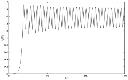
FIG. 1.: Time evolution of $\omega_{\rm b}(t)/\gamma_{\rm r}$ for the cold beam instability. The initial velocity of the beam was chosen to maximize $\gamma_{\rm r}$ and the beam is initially spatially homogeneous.

FIG. 2.: Snapshots of the $(x,p)$ space at (a) $\gamma_{\rm r}t=6.24$, (b) $\gamma_{\rm r}t=17.5$, (c) $\gamma_{\rm r}t=100$ for the cold beam simulation of Fig. 1. Dots are the $N=10000$ particles, which were initially distributed on a monokinetic beam, faster than the wave (with very small initial intensity). The instantaneous wave resonance ‘cat eye’ is drawn to help in visualizing the instantaneous force on particles.

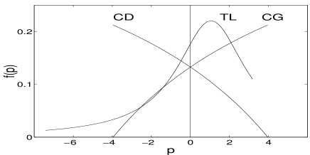
FIG. 3.: Initial warm beam velocity distributions.

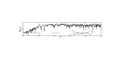
FIG. 4.: Time evolution of $\ln(\omega_{\rm b}(t)/|\gamma_{\rm L}|)$ for a CD velocity distribution and initial wave amplitude below thermal level : (N) $N$-particles system with $N=32000$, (V) kinetic scheme with $32\times 512$ $(x,p)$ grid. Inset : short-time evolution.

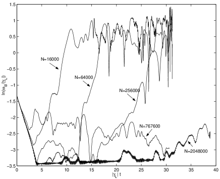
FIG. 5.: Time evolution of $\ln(\omega_{\rm b}(t)/|\gamma_{\rm L}|)$ for an initial CD velocity distribution and different values of $N$. When necessary for readability, curves were smoothed through a sliding window average.

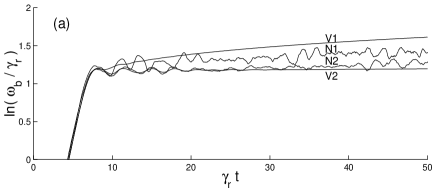
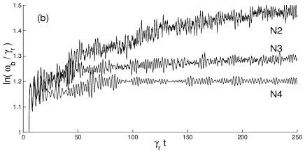
FIG. 6.: Time evolution of $\ln(\omega_{\rm b}(t)/\gamma_{\rm r})$. (a) CG initial distribution : kinetic scheme with (V1) $32\times 128$, (V2) $256\times 1024$ $(x,p)$ grid ; $N$-particles system with (N1) $N=128000$, (N2) $N=512000$ ; (b) Comparison of CG (N2) with TL initial distribution for (N3) $N=64000$, (N4) $N=2048000$.

FIG. 7.: Coefficients $a_{n}/a_{0}$ ($n\geq 1$) of the Fourier decomposition of amplitude $\omega_{\rm b}^{2}(t)$ during the first time window $38\leq\gamma_{\rm L}t\leq 65$ for $N=48000$ (solid curve) and $N=768000$ (dashed curve) particles, as a function of normalized frequency.

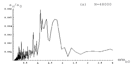
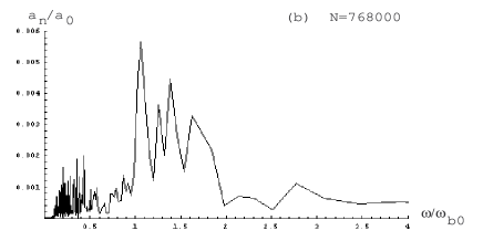
FIG. 8.: Coefficients $a_{n}/a_{0}$ ($n\geq 1$) of the Fourier decomposition of amplitude $\omega_{\rm b}^{2}(t)$ during the second time window $250\leq\gamma_{\rm L}t\leq 302$ as a function of normalized frequency, for (a) $N=48000$ and for (b) $N=768000$ particles.

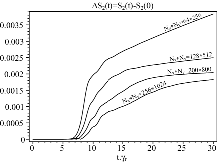
FIG. 9.: Evolution of the 2-entropy $S_{2}=\int(1-f)fdxdp$ as a function of time $\gamma_{\rm r}t$ in the Vlasov simulations for several $N_{x}\times N_{v}$ grids. The departure from zero indicates that the damping of trapping oscillations is spurious.

REFERENCES

- [1] Email : X@newsup.univ-mrs.fr (X = firpo, doveil, elskens), Pierre.Bertrand@lpmi.uhp-nancy.fr
- [2] M. Antoni, Y. Elskens and D.F. Escande, Phys. Plasmas 5, 841 (1998).
- [3] J.D. Crawford and A. Jayaraman, Phys. Plasmas 6, 666 (1999).
- [4] D. del-Castillo-Negrete, Phys. Lett. A 241, 99 (1998), Phys. Plasmas 5, 3886 (1998), Physica A 280, 10 (2000), Chaos 10, 75 (2000).
- [5] M-C. Firpo and Y. Elskens, J. Stat. Phys. 93, 193 (1998); Phys. Scripta T75, 169 (1998).
- [6] G. Brodin, Phys. Rev. Lett. 78, 1263 (1997); G. Manfredi, ibid. 79, 2815 (1997); M.B. Isichenko, ibid. 78, 2369 (1997), 80, 5237 (1998); C. Lancellotti and J.J. Dorning, ibid. 80, 5236 (1998), 81, 5137 (1998).
- [7] M. Brunetti, F. Califano and F. Pegoraro, Phys. Rev. E 62, 4109 (2000).
- [8] L.D. Landau, J. Phys. USSR 10, 25 (1946); J.H. Malmberg and C.B. Wharton, Phys. Rev. Lett. 6, 184 (1964); D.D. Ryutov, Plasma Phys. Control. Fusion 41, A1 (1999).
- [9] T.M. O’Neil, Phys. Fluids 8, 2255 (1965).
- [10] B.D. Fried et al., Plasma Physics Group Report PPG-93, University of California, Los Angeles, 1971 (unpublished); A. Simon and M.N. Rosenbluth, Phys. Fluids 19, 1567 (1976); P.A.E.M. Janssen and J.J. Rasmussen, Phys. Fluids 24, 268 (1981); J.D. Crawford, Phys. Rev. Lett. 73, 656 (1994).
- [11] H.E. Mynick and A.N. Kaufman, Phys. Fluids 21, 653 (1978).
- [12] J.L. Tennyson, J.D. Meiss and P.J. Morrison, Physica D 71, 1 (1994).
- [13] W.E. Drummond et al., Phys. Fluids 13, 2422 (1970); T.M. O’Neil, J.H. Winfrey and J.H. Malmberg, Phys. Fluids 14, 1204 (1971); T.M. O’Neil and J.H. Winfrey, Phys. Fluids 15, 1514 (1972); I.N. Onischenko et al., Pis’ma Zh. Eksp. Teor. Fiz. 12, 407 (1970) [JETP Lett. 12, 281 (1970)].
- [14] J.R. Cary and I. Doxas, J. Comput. Phys. 107, 98 (1993); J.R. Cary et al., Phys. Fluids B 4, 2062 (1992); I. Doxas and J.R. Cary, Phys. Plasmas 4, 2508 (1997).
- [15] D.F. Escande, S. Zekri and Y. Elskens, Phys. Plasmas 3, 3534 (1996); S. Zekri, Ph.D. thesis (Marseille, 1993).
- [16] S.I. Tsunoda, F. Doveil and J.H. Malmberg, Phys. Rev. Lett. 59, 2752 (1987).
- [17] G. Laval and D. Pesme, Phys. Rev. Lett. 53, 270 (1984); Plasma Phys. Control. Fusion 41, A239 (1999).
- [18] P. Bertrand et al., Phys. Fluids B 4, 3590 (1992); E. Sonnendrücker et al., J. Comput. Phys. 151, 201 (1999).
- [19] F. Doveil et al., Phys. Lett. A (2001), in press.
- [20] Y. Kuramoto, Chemical Oscillations, Waves and Turbulence, Springer, Berlin, 1984.
- [21] M-C. Firpo and Y. Elskens, Phys. Rev. Lett. 84, 3318 (2000).
- [22] M-C. Firpo, Ph.D. thesis (Marseille, 1999); preprint.
- [23] N.G. van Kampen, Physica 21, 949 (1955), 23, 641 (1957) ; K.M. Case, Ann. Physics 7, 349 (1959).
- [24] D. Guyomarc’h, Ph.D. thesis (Marseille, 1996); D. Guyomarc’h et al., in Transport, Chaos and Plasma Physics 2, S. Benkadda, F. Doveil and Y. Elskens eds (World Scientific, Singapore, 1996) pp. 406-410; Y. Elskens, D. Guyomarc’h and M-C. Firpo, Physicalia Mag. 20, 193 (1998).
- [25] M.R. Feix, P. Bertrand and A. Ghizzo, in Advances in Kinetic Theory and Computing, B. Perthame ed. (World Scientific, Singapore, 1994) pp. 45-81.
- [26] I.B. Bernstein, J.M. Greene and M.D. Kruskal, Phys. Rev. 108, 546 (1957); J.P. Holloway and J.J. Dorning, Phys. Rev. A 44, 3856 (1991); M. Buchanan and J.J. Dorning, Phys. Rev. E 52, 3015 (1995).
- [27] V. Latora, A. Rapisarda and S. Ruffo, Phys. Rev. Lett. 80, 692 (1998).
- [28] For any finite , the only exact self-consistent solutions of (3)-(4) with time-independent field (i.e. analogue of BGK modes [26]) have constant zero field (Y. Elskens, submitted for publication).
- [29] Y. Elskens and D.F. Escande, Nonlinearity 4, 615 (1991); Physica D 62, 66 (1992).
- [30] D.F. Escande, Phys. Rep. 121, 165 (1985).
- [31] With (21), the force (19) reads .
- [32] J.D. Meiss, Physica D 74, 254 (1994).