Generic Smooth Connection Functions
A New Analytic Approach to Interpolation

Abstract

We present a generic solution to the fundamental problem of how to connect two points in a plane by a smooth curve that goes through these points with a given slope. The smoothness of any curve depends both on its curvature and its length. The smoothest curves correspond to a particular compromise between minimal curvature and minimal length. They can be described by a class of functions that satisfy certain boundary conditions and minimize a weight functional. The value of this functional is given essentially by the average of the curvature raised to some power $\nu$ times the length of the curve. The parameter $\nu$ determines the importance of minimal curvature with respect to minimal length. In order to find the functions that obtain the minimal weight, we use extensively notions that are well-known in classical mechanics. The minimization of the weight functional via the Euler-Lagrange formalism leads to a highly non-trivial differential equation. Using the symmetries of the problem it is possible to find conserved quantities, that help to simplify the problem to a level where the solution functions can be written in a closed form for any given $\nu$. Applying the appropriate coordinate transformation to these solutions allows to adjust them to all possible boundary conditions.

I Introduction

A The problem

Consider two points in a plane, each associated with a ray pointing in some direction. The problem we address in this paper is how to connect these points in a “smooth” way. That is we are looking for a curve that satisfies the following three conditions:

1. The curve goes through both points.

2. The associated ray at each point is a tangent to the curve.

3. Between the two points the curve follows some optimal path, which is a compromise between minimal curvature and minimal length.

The first two requirements constitute the boundary conditions of the problem. The third condition defines what we mean by “smooth”.

B Motivation and Outline

A solution to the problem outlined above has many obvious applications. For example it could be used to determine the ideal shape of a road to be built between two points where its direction is predetermined (e.g. by two bridges). In fact any interpolation problem that has been reduced to the task of connecting a sample of data points where the slope is fixed can be solved using the elementary solution of connecting smoothly two points. If the original sample only consists of points, the respective slopes can be determined, for example, by taking the slope of the line through the neighboring points, or by some different, more sophisticated method. Evidently the quality of interpolation curves is crucial to all fields that deal with numerical data from applied sciences to economics. It is interesting to note that while there exist many interpolation schemes, most of them rely on simple functions, like polynomials, that in general do not give the best interpolation. The aim of this work is to establish first a criterion for the quality of the interpolation and then to investigate quantitatively which are the optimal interpolating curves.

As we shall see in the following, the problem outlined above translates into a well-defined mathematical exercise, which is interesting by itself. In fact we feel that our solution to the problem, relying heavily on notions well known in physics, has also a pedagogical value. It serves as an example of some fundamental physics principles in the context of a very intuitive and visual, yet non-trivial problem.

Since the problem is defined as a geometrical task, its mathematical formulation obviously does not depend on time. Instead we take one space-direction ($x$) as the variable of integration, and the other space-direction ($y$) to describe the solution function. While this description is not manifestly invariant under rotations and translations in the $x-y$ plane, it allows us to define an action functional that assigns a weight to any function (that complies with the boundary conditions) according to its “smoothness”. It is given essentially by the average of the inverse curvature radius, to some power $\nu$, times the length of the curve. This action is minimized by a class of functions, each describing the smoothest curve for a particular choice of the parameter $\nu$ that specifies the relative importance of minimal curvature with respect to minimal length. These functions are the solutions of the Euler-Lagrange equation, which turns out to be a complicated, non-linear third order differential equation. Solving this equation can be facilitated immensely by taking advantage of the symmetries of the problem. We compute the linear and angular momenta that follow from Noether’s theorem due to the translational and rotational invariance. The equation of motion is also scale invariant, but there exists no conserved charge corresponding to scaling, since the Lagrangian and other dimensionful variables do change under scaling transformations. The problem is solved explicitly for a particular choice of the momenta. Applying the appropriate coordinate transformation to this solution allows to adjust it to all possible boundary conditions.

II Formalism

In order to translate the problem outlined in Section I A into a mathematical one we have to introduce some notations: Let us give “names” to the two points: We shall refer to them as the initial point $P_{i}$ and the final point $P_{f}$. Which one is which is arbitrary, but when introducing coordinates

$$P_{i}:(x_{i},y_{i})~{}~{}~{}~{}~{}~{}\mbox{and}~{}~{}~{}~{}~{}~{}P_{f}:(x_{f},y_{f})\,,$$ (1)

we demand that $x_{i}<x_{f}$. The coordinates $(x,y)$ are a set of two real numbers specifying any point in the plane. We use simple Euclidean geometry. The associated rays at $P_{i}$ and $P_{f}$ are described by their inclination angles, $\alpha_{i}$ and $\alpha_{f}$, with respect to the vector pointing from $P_{i}$ to $P_{f}$ (c.f. Fig. 1).

We call the function $y(x)$ that satisfies the three conditions in Section I A the “smooth connection function” (SCF). Our task is to determine this function. The boundary conditions defined in Section I A are:

$$y(x_{i}) = y_{i}~{}~{}~{}~{}~{}~{}~{}~{}~{}~{}~{}~{}~{}~{}~{}~{}~{}~{}~{}~{}~{}\mbox{and}~{}~{}~{}~{}~{}~{}~{}y(x_{f})=y_{f}\,,$$ (2)

$$y^{\prime}(x_{i}) = \tan(\alpha_{i}+\alpha_{0})~{}~{}~{}~{}~{}~{}~{}\mbox{and}~{}~{}~{}~{}~{}~{}\,y^{\prime}(x_{f})=\tan(\alpha_{f}+\alpha_{0})\,,$$ (3)

where the prime denotes a derivative with respect to $x$ and $\alpha_{0}$ is the angle between the positive $x$-axis and the vector pointing from $P_{i}$ to $P_{f}$.

In order to include the third and crucial condition in Section I A we need to incorporate both the curvature and the length of the curve. The local curvature at a given point on the curve is defined as the inverse radius $(1/r)$ of the circle that coincides with the curve in the infinitesimal vicinity of the point. It is given in terms of the first and second derivative of the function $y(x)$ by:

$${1\over r(x)}={|y^{\prime\prime}(x)|\over[1+y^{\prime}(x)^{2}]^{3/2}}\,.$$ (4)

To show this relation it is enough to verify that the curves that describes a circle, i.e. $y(x)=\pm\sqrt{r^{2}-(x-x_{0})^{2}}+y_{0}$, where $r$ is the radius and $(x_{0},y_{0})$ denotes the center of the circle, give $r(x)=r$. The length of an infinitesimal piece of the curve at $x$ is given by

$$ds(x)=\sqrt{1+y^{\prime}(x)^{2}}\,dx\,.$$ (5)

We define now the following functional:

$$\tilde{\cal S}[y(x)]\equiv\int_{x_{i}}^{x_{f}}\left({1\over r(x)}\right)^{\nu}\,ds(x)=\int_{x_{i}}^{x_{f}}{|y^{\prime\prime}(x)|^{\nu}\over\left[1+y^{\prime}(x)^{2}\right]^{3\nu-1\over 2}}\,dx\,.$$ (6)

We shall refer to $\tilde{\cal S}[y(x)]$ as the action. For a given function $y(x)$ it returns the weighted sum of $ds(x)$ where $x$ goes from $x_{i}$ to $x_{f}$. The weight at position $x$ is given by the local curvature $1/r(x)$, defined in eq. (4), raised to some power $\nu$. A priori this parameter is an arbitrary real number that determines how to choose the compromise between minimal curvature and minimal length. For example, for $\nu=0$ the curvature does not play a role at all and $\tilde{\cal S}[y(x)]_{\nu=0}$ is just the length of the curve. For $|\nu|\to\infty$ the situation is exactly the opposite, since $\tilde{\cal S}[y(x)]_{|\nu|\to\infty}\simeq\int(1/r)^{\nu}dx$ only depends on the curvature in this case. A special situation arises for $\nu=1$, where $\tilde{\cal S}[y(x)]=\int_{x_{i}}^{x_{f}}(ds/r)=\int_{x_{i}}^{x_{f}}d\alpha=\alpha_{f}-\alpha_{i}$. Since the action gives just the difference between the inclination angles at the boundary, independent of the particular choice of $y(x)$, it is impossible to determine the optimal path for $\nu=1$ and we exclude this case from our subsequent discussion.

In order to find the optimal curve we have to minimize the action under the boundary conditions in eq. (2) and eq. (3). Before we continue with our analysis we would like to give a concrete example illustrating the relevance of the action functional. Consider a spacecraft that has been launched to explore some distant planets and which is flying with constant velocity $v$ through the interstellar space. When approaching a certain planet, one has to adjust carefully the trajectory of the spaceship, say to enter the atmosphere of the planet at a precise angle or to use its gravitational field to accelerate the spacecraft to its next destination. Suppose that for this purpose the spaceship has thrusters that exert a force $F$ perpendicular to the direction of motion. Then at any given time $t$ between the ignition (at $t_{i}$) and the end of the manoeuvre (at $t_{f}$) the instantaneous curvature radius $r(t)$ is inversely proportional to $F$. Let us assume that the fuel consumption per unit time, ${\cal W}$, is governed by some potential law, i.e. ${\cal W}\propto F^{\nu}\propto(1/r)^{\nu}$, where $\nu$ is an empirical parameter. Then the total fuel consumption, ${\cal C}=\int_{t_{i}}^{t_{f}}{\cal W}dt$, is proportional to the action in eq. (6), since $dt=ds/v$. Obviously minimizing ${\cal C}$ is crucial. Once we have found the solution for the trajectory we can obtain the curvature radius as a function of $t$ which indicates how much fuel should be burned at each point.

The integrand in eq. (6), usually referred to as the Lagrangian,

$$\tilde{\cal L}(y^{\prime},y^{\prime\prime})\equiv{|y^{\prime\prime}(x)|^{\nu}\over\left[1+y^{\prime}(x)^{2}\right]^{3\nu-1\over 2}}$$ (7)

only depends on $y^{\prime}(x)$ and $y^{\prime\prime}(x)$, while there is no explicit dependence on $y(x)$ and $x$. Thus $y$ and $x$ enter the action $\tilde{\cal S}[y(x)]$ only via the boundary conditions. From eq. (2) it follows that

$$y_{f}-y_{i}=y(x_{f})-y(x_{i})=\int_{x_{i}}^{x_{f}}y^{\prime}(x)=constant\,.$$ (8)

This constraint can be absorbed into the action functional by introducing a Lagrange multiplier $\lambda$, resulting in a new action

$${\cal S}[y^{\prime}(x)]\equiv\tilde{\cal S}[y^{\prime}(x)]+\lambda\int_{x_{i}}^{x_{f}}y^{\prime}(x)=\int_{x_{i}}^{x_{f}}\left[\tilde{\cal L}+\lambda\,y^{\prime}(x)\right]\,dx\,.$$ (9)

Since there is no reference to $y(x)$ anymore, but only to its first and second derivative, we can change variables,

$$q(x)=y^{\prime}(x)~{}~{}~{}~{}~{}~{}\mbox{and}~{}~{}~{}~{}~{}~{}q^{\prime}(x)=y^{\prime\prime}(x)\,,$$ (10)

and write the Lagrangian corresponding to the action ${\cal S}[q(x)]$ in eq. (9) as

$${\cal L}(q,q^{\prime})\equiv\tilde{\cal L}(q,q^{\prime})+\lambda\,q(x)={|q^{\prime}|^{\nu}\over\left(1+q^{2}\right)^{3\nu-1\over 2}}+\lambda\,q\,.$$ (11)

Now, to minimize $\tilde{\cal S}[y(x)]$ under the boundary condition in eq. (2) is equivalent to the minimization of ${\cal S}[q(x)]$. A necessary condition for ${\cal S}[q(x)]$ to be extremal is that its first functional derivative $\delta{\cal S}[q(x)]/\delta q(x)$ vanishes. Since ${\cal S}[q(x)]$ only depends on $q$ and $q^{\prime}$, this is a well-known problem. Its solution is given by the Euler-Lagrange equation:

$${\partial{\cal L}\over\partial q}-{d\over dx}\,{\partial{\cal L}\over\partial q^{\prime}}=0\,.$$ (12)

Computing

$${\partial{\cal L}\over\partial q} = {(1-3\nu)|q^{\prime}|^{\nu}q\over\left(1+q^{2}\right)^{3\nu+1\over 2}}+\lambda\,,$$ (13)

$${\partial{\cal L}\over\partial q^{\prime}} = {\nu\,\sigma|q^{\prime}|^{\nu-1}\over\left(1+q^{2}\right)^{3\nu-1\over 2}}\,,$$ (14)

$${d\over dx}\,{\partial{\cal L}\over\partial q^{\prime}} = {\nu(\nu-1)|q^{\prime}|^{\nu-2}q^{\prime\prime}\over\left(1+q^{2}\right)^{3\nu-1\over 2}}+{\nu(1-3\nu)|q^{\prime}|^{\nu}q\over\left(1+q^{2}\right)^{3\nu+1\over 2}}\,,$$ (15)

where $\sigma\equiv{\rm sign}(q^{\prime})$, we obtain

$$\lambda={(\nu-1)|q^{\prime}|^{\nu-2}\over\left(1+q^{2}\right)^{3\nu+1\over 2}}\left[\nu(1+q^{2})q^{\prime\prime}+(1-3\nu)(q^{\prime})^{2}q\right]\,.$$ (16)

The above equation still depends on the parameter $\lambda$. We can eliminate this dependence by differentiating eq. (16) with respect to $x$ yielding the following equation of motion (EOM)

$$0={(\nu-1)|q^{\prime}|^{\nu-3}\over\left(1+q^{2}\right)^{3\nu+3\over 2}} \left\{(1-3\nu)\left[(1-3\nu q^{2})(q^{\prime})^{4}+2\nu q(1+q^{2})(q^{\prime})^{2}q^{\prime\prime}\right]\right.+$$ (17)

$$\left.~{}~{}\nu(1+q^{2})^{2}\left[(\nu-2)(q^{\prime\prime})^{2}+q^{\prime}q^{\prime\prime\prime}\right]\right\}\,.$$ (18)

For all functions $q(x)$ that solve the above EOM the action ${\cal S}[q(x)]$ in eq. (9) is stationary, i.e. $\delta{\cal S}[q(x)]/\delta q(x)=0$. However, in order to minimize ${\cal S}[q(x)]$ also the so-called Legendre condition,

$$0<{\partial^{2}{\cal L}\over(\partial q^{\prime})^{2}}={\nu(\nu-1)|q^{\prime}|^{\nu-2}\over\left(1+q^{2}\right)^{3\nu-1\over 2}}\,,$$ (19)

has to be satisfied. This condition arises from the second functional variation of the action with respect to $q(x)$. Note that unlike for the minimization of usual functions it is only a necessary condition for a minimum of ${\cal S}[q(x)]$. This is essentially because a small variation in $q$ does not necessarily imply a small variation in $q^{\prime}$. However in our case the sign of ${\partial^{2}{\cal L}/(\partial q^{\prime})^{2}}$ only depends on the prefactor $\nu(\nu-1)$, but is independent of $q$ and $q^{\prime}$ even if they are taken as independent variables. Such a situation is referred to as a “regular problem” and it implies that the solutions of the EOM indeed give rise to a local minimum of the action if $\nu<0$ or $\nu>1$. Conversely for $0<\nu<1$ one obtains a local maximum. Thus we rule out any $0<\nu\leq 1$ from our analysis and we shall only consider $\nu\leq 0$ and $\nu>1$ from now on.

Even though we have managed to translate the problem at hand into a differential equation, solving this equation analytically seems like a formidable task given that eq. (17) is third order in $q$ and non-linear. However, the integrated form in eq. (16) gives us a hint of how to proceed. The fact that $\lambda$ is a constant is related to the symmetries inherent to the problem. Studying these symmetries systematically one can simplify the problem significantly and find its solutions.

III Symmetries

Let us examine more carefully the problem with respect to its intrinsic symmetries. The important point to realize is that when introducing the coordinates in eq. (1) we have made an explicit choice of

• where to define the origin,

• how to orientate the axes and

• what units of length to use.

These choices are arbitrary and once we have found a solution to our problem we can redefine our coordinate system. Assume that $y(x)$ solves the EOM in eq. (17) in some coordinate system $\Sigma$ and that $\tilde{y}(\tilde{x})$ is obtained from $y(x)$ by a transformation to a different coordinate system $\tilde{\Sigma}$ ,

$$\pmatrix{x\cr y}\to\pmatrix{\tilde{x}\cr\tilde{y}}={\bf R}\pmatrix{x\cr y}+\pmatrix{x_{0}\cr y_{0}}\,,$$ (20)

where

$${\bf R}\equiv\pmatrix{\cos\theta&-\sin\theta\cr\sin\theta&\cos\theta}$$ (21)

describes a rotation by an angle $\theta$, and $x_{0}$ and $y_{0}$ parameterize a translation in the $x$-direction and in the $y$-direction, respectively. The action in eq. (6) is defined in terms the curvature radius $r$ [c.f. eq. (4)] and the length element $ds$ in eq. (5). Both quantities are manifestly invariant under rotations and translations. Therefore it is clear that the coordinate transformations in eq. (20) do not change the action nor the EOM derived from it. However the boundary conditions obviously have to change under $\Sigma\to\tilde{\Sigma}$.

Let us consider the infinitesimal change of the coordinate $y$ at a given $x$,

$$\delta y(x)\equiv\tilde{y}(x)-y(x)\,,$$ (22)

for the three types of coordinate transformations. For a translation in the $y$-direction

$$y_{0}=\epsilon_{y}\ll 1\,,~{}~{}~{}~{}~{}x_{0}=0\,,~{}~{}~{}~{}~{}\theta=0\,,$$ (23)

the answer is trivial. The change in $y$ is simply

$$\delta y(x,\epsilon_{y})=\epsilon_{y}\,,$$ (24)

implying that the changes in all the derivatives of $y(x)$ vanish:

$$\delta q(x,\epsilon_{y}) = 0\,,$$ (25)

$$\delta q^{\prime}(x,\epsilon_{y}) = 0\,,$$ (26)

$$\delta q^{\prime\prime}(x,\epsilon_{y}) = 0\,.$$ (27)

However, a translation in the $x$-direction

$$y_{0}=0\,,~{}~{}~{}~{}~{}x_{0}=\epsilon_{x}\ll 1\,,~{}~{}~{}~{}~{}\theta=0\,,$$ (28)

is a bit more tricky. First, note that

$$\tilde{y}(\tilde{x})=y(x)\,.$$ (29)

This expresses merely the fact that the coordinate transformation in eq. (20) leaves the functional behavior of $y(x)$ invariant. It does not make a difference whether we refer to the function by $y(x)$ in the coordinate system $\Sigma$ or $\tilde{y}(\tilde{x})$ in the system $\tilde{\Sigma}$. Then a Taylor expansion of $\tilde{y}(\tilde{x})$ around $x$ gives

$$\tilde{y}(\tilde{x})=\tilde{y}(x)+\left.{\partial y\over\partial x}\right|_{x}\,\epsilon_{x}\,,$$ (30)

implying that

$$\delta y(x,\epsilon_{x})=-\left.{\partial y\over\partial x}\right|_{x}\,\epsilon_{x}\,.$$ (31)

From eq. (31) it follows that the corresponding changes in the derivatives of $y(x)$ are given by

$$\delta q(x,\epsilon_{x}) = -q^{\prime}(x)\,\epsilon_{x}\,,$$ (32)

$$\delta q^{\prime}(x,\epsilon_{x}) = -q^{\prime\prime}(x)\,\epsilon_{x}\,,$$ (33)

$$\delta q^{\prime\prime}(x,\epsilon_{x}) = -q^{\prime\prime\prime}(x)\,\epsilon_{x}\,.$$ (34)

Finally, an infinitesimal rotation

$$y_{0}=0\,,~{}~{}~{}~{}~{}x_{0}=0\,,~{}~{}~{}~{}~{}\theta=\epsilon_{\theta}\,,$$ (35)

involves both a change in $x$ by $-y\epsilon_{\theta}$ and in $y$ by $x\epsilon_{\theta}$. Together this results into a change of $y(x)$ by:

$$\delta y(x,\epsilon_{\theta})=\left(x+\left.{\partial y\over\partial x}\right|_{x}y\right)\,\epsilon_{\theta}\,.$$ (36)

From eq. (36) it follows that the changes in $q$, $q^{\prime}$ and $q^{\prime\prime}$ for an infinitesimal rotation are given by

$$\delta q(x,\epsilon_{\theta}) = (1+q^{2}+yq^{\prime})\,\epsilon_{\theta}\,,$$ (37)

$$\delta q^{\prime}(x,\epsilon_{\theta}) = (3qq^{\prime}+yq^{\prime\prime})\,\epsilon_{\theta}\,,$$ (38)

$$\delta q^{\prime\prime}(x,\epsilon_{\theta}) = (3(q^{\prime})^{2}+4qq^{\prime\prime}+yq^{\prime\prime\prime})\,\epsilon_{\theta}\,.$$ (39)

Let us now investigate the effect of the coordinate transformations in eq. (20) on the Lagrangian ${\cal L}$ in eq. (11). In general an infinitesimal transformation parameterized by $\epsilon\ll 1$ will induce a change

$$\delta{\cal L}\equiv{\cal L}(\tilde{q},\tilde{q}^{\prime})-{\cal L}(q,q^{\prime})\,.$$ (40)

Provided that ${\cal L}$ has no explicit dependence on $x$, a Taylor expansion of ${\cal L}(\tilde{q},\tilde{q}^{\prime})$ around $q$ gives

$$\delta{\cal L} = {\partial{\cal L}\over\partial q}\delta q+{\partial{\cal L}\over\partial q^{\prime}}\delta q^{\prime}$$ (41)

$$= {d\over dx}\left({\partial{\cal L}\over\partial q^{\prime}}\delta q\right)+\left({\partial{\cal L}\over\partial q}-{d\over dx}\,{\partial{\cal L}\over\partial q^{\prime}}\right)\delta q\,.$$ (42)

The second term in eq. (42) vanishes for $q(x)$ that satisfy the equation of motion (12).

Any transformation that changes the action ${\cal S}[q(x)]$ in eq. (9) at most by constant is called a symmetry transformation. Such a transformation does not change the extremal condition for the action and therefore leaves the EOM invariant. (Note however that not all transformations that leave the EOM unchanged are symmetry transformations according to our definition.) Then, the corresponding Lagrangian could change only by a total derivative:

$$\delta{\cal L}=\epsilon{dF\over dx}\,,$$ (43)

where $F(q,q^{\prime})$ is a function of $q$ and $q^{\prime}$. Equating the two results for $\delta{\cal L}$ we find that

$$\epsilon{dF\over dx}={d\over dx}\left({\partial{\cal L}\over\partial q^{\prime}}\delta q\right)\,.$$ (44)

We stress that the expression on the left-hand side is correct for a symmetry transformation of any function $y(x)$, while the right-hand side is only valid for a transformation of $y(x)$ that solves the EOM. From eq. (44) it follows that the conserved charge defined as

$$Q=F-{\partial{\cal L}\over\partial q^{\prime}}{\delta q\over\epsilon}$$ (45)

is a constant with respect to $x$, i.e. $dQ/dx=0$. Consequently it has one specific value for all points on a particular solution of the EOM. Obviously $Q$ can only be defined up to a constant. The above argument, that every continuous symmetry transformation implies a conserved charge is known as the Noether theorem.

To be explicit let us apply it to a translation in the $x$ direction. Using eq. (32) it follows that

$$\delta{\cal L}(x,\epsilon_{x}) = -\left({\partial{\cal L}\over\partial q}q^{\prime}+{\partial{\cal L}\over\partial q^{\prime}}q^{\prime\prime}\right)\,\epsilon_{x}$$ (46)

$$= -{d{\cal L}\over dx}\epsilon_{x}\,.$$ (47)

This means that (up to a constant) we can identify $F_{x}=-{\cal L}$. Then it follows that the conserved charge corresponding to translations in the $x$ direction is given by:

$$P_{x} = {\partial{\cal L}\over\partial q^{\prime}}q^{\prime}-{\cal L}$$ (48)

$$= {{(\nu-1)|q^{\prime}|^{\nu}}\over{\left(1+q^{2}\right)^{3\nu-1\over 2}}}-\lambda\,q\,.$$ (49)

We call $P_{x}$ the conserved momentum in the $x$ direction. In fact it is nothing more than the Legendre transformation of the Lagrangian with respect to $q^{\prime}$. (If the variable of integration in eq. (9) had been the time $t$ rather the coordinate $x$ then the equivalent Legendre transformation of the Lagrangian with respect to $dq/dt$ is called the Hamiltonian and the charge related to time invariance is the energy.)

One might guess that a similar argument for translations in the $y$ direction should give another conserved charge $P_{y}$, which is the conserved momentum in the $y$ direction. However a change in the variable $y(x)$ as in eq. (24) has no effect on $q(x)$ and $q^{\prime}(x)$, see eq. (25), implying trivially that

$$\delta{\cal L}(x,\epsilon_{y})=0\,.$$ (50)

Thus Noether’s theorem does not help in this case to derive the conserved charge. However we have already encountered another conserved quantity, which could serve as a candidate for $P_{y}$. In order to absorb the boundary condition into the action we introduced the Lagrange multiplier $\lambda$, which intuitively is related to changes in $y$, c.f. eq. (9). Eq. (16) states that $\lambda$ equals to a complicated function of $q$, $q^{\prime}$ and $q^{\prime\prime}$ for all $x$. Therefore this function is a constant of motion. To prove that indeed $P_{y}=\lambda$ is nontrivial and we will show this after discussing the conserved charge related to the rotations in eq. (20).

Using eqs. (13) and (14) and the changes in $q$ and $q^{\prime}$ under rotations according to eq. (37) the change in the Lagrangian under an infinitesimal rotation is

$$\delta{\cal L}(x,\epsilon_{\theta})=\left\{\left[{(1-3\nu)|q^{\prime}|^{\nu}q\over\left(1+q^{2}\right)^{3\nu+1\over 2}}+\lambda\right]\,(1+q^{2}+yq^{\prime})+\left[{\nu|q^{\prime}|^{\nu-1}\over\left(1+q^{2}\right)^{3\nu-1\over 2}}\right]\,(3qq^{\prime}+yq^{\prime\prime})\right\}\epsilon_{\theta}\,.$$ (51)

It is not difficult to check that this can be rewritten as a total derivative,

$$\delta{\cal L}(x,\epsilon_{\theta})={d\over dx}\left[{y|q^{\prime}|^{\nu}\over\left(1+q^{2}\right)^{3\nu-1\over 2}}+\lambda(x+yq)\right]\epsilon_{\theta}\,.$$ (52)

Thus for infinitesimal rotations the function $F$ can be identified to be (up to a constant)

$$F_{\theta}=y{\cal L}+x\lambda\,.$$ (53)

Then the charge corresponding to the rotation symmetry, which is called the total angular momentum, is given by

$$J = F_{\theta}-{\partial{\cal L}\over\partial q^{\prime}}{\delta q(x,\epsilon_{\theta})\over\epsilon_{\theta}}$$ (54)

$$= y{\cal L}+x\lambda-{\nu\,\sigma|q^{\prime}|^{\nu-1}\over\left(1+q^{2}\right)^{3\nu-1\over 2}}\,(1+q^{2}+yq^{\prime})$$ (55)

$$= \left(xP_{y}-yP_{x}\right)+S\,.$$ (56)

In the last step we have separated the total angular momentum into the orbital contribution

$$L=xP_{y}-yP_{x}$$ (57)

and the remaining term

$$S=-{\nu\,\sigma|q^{\prime}|^{\nu-1}\over\left(1+q^{2}\right)^{3\nu-3\over 2}}=-{\nu\,\sigma\over[r(x)]^{\nu-1}}\,,$$ (58)

which we call the spin or intrinsic angular momentum. The orbital angular momentum would be the sole contribution if $y(x)$ is a straight line (as is the case for $\nu=0$ or if $q^{\prime}=0$). A non-vanishing spin $S$ arises for all the other curves due to their curvature. Note that it is sensitive to the sign $\sigma$ of $q^{\prime}$.

We would like to come back now to our claim that $P_{y}$ coincides with $\lambda$ defined in eq. (16). To this end let us compute the change in $P_{i}~{}~{}(i=x,y)$ induced by rotations. In general

$$\delta P_{i}(x,\epsilon_{\theta})=\left[{\partial P_{i}\over\partial q}(1+q^{2})+{\partial P_{i}\over\partial q^{\prime}}(3qq^{\prime})+{\partial P_{i}\over\partial q^{\prime\prime}}(3[q]^{2}+4qq^{\prime\prime})\right]\epsilon_{\theta}\,,$$ (59)

where we used the results in eq. (37) and the fact that the terms proportional to $y$ add up to the total derivative of $P_{i}$:

$$y\left[{\partial P_{i}\over\partial q}q^{\prime}+{\partial P_{i}\over\partial q^{\prime}}q^{\prime\prime}+{\partial P_{i}\over\partial q^{\prime\prime}}q^{\prime\prime\prime}\right]\epsilon_{\theta}=y{dP_{i}\over dx}\epsilon_{\theta}=0\,.$$ (60)

Assuming that indeed $P_{y}=\lambda$, a somewhat tedious but straight-forward calculation of $\delta P_{y}$ according to eq. (59) yields

$$\delta P_{y}(x,\epsilon_{\theta})={(\nu-1)|q^{\prime}|^{\nu-2}\over\left(1+q^{2}\right)^{3\nu+1\over 2}}\left[(1+3\nu q^{2})(q^{\prime})^{2}-\nu q(1+q^{2})q^{\prime\prime}\right]\epsilon_{\theta}=P_{x}\epsilon_{\theta}\,.$$ (61)

Similarly using eq. (59) one shows that $\delta P_{x}(x,\epsilon_{\theta})=-P_{y}\epsilon_{\theta}$. From the infinitesimal transformations it is clear that ${\bf P}=(P_{x},P_{y})$ transforms like a vector under rotations, i.e. $\tilde{\bf P}={\bf R}\cdot{\bf P}$, where ${\bf R}$ is the rotation matrix defined in eq. (21). It follows that the constant $\lambda$ in eq. (16) can indeed be identified with the conserved momentum in the $y$-direction.

Using the above results it is easy to compute the change in the orbital angular momentum $L$ under infinitesimal rotations:

$$\delta L(x,\epsilon_{\theta}) = x\cdot\delta P_{y}(x,\epsilon_{\theta})-\left[\delta y\cdot P_{x}(x,\epsilon_{\theta})+y\cdot\delta P_{x}(x,\epsilon_{\theta})\right]$$ (62)

$$= -y(qP_{x}-P_{y})\epsilon_{\theta}$$ (63)

Note that this is the change at a fixed $x$, so of course there is no variation with respect to $x$. The change in the spin $S$ under rotations is given by

$$\delta S(x,\epsilon_{\theta}) = {\partial S\over\partial q}\delta q(x,\epsilon_{\theta})+{\partial S\over\partial q^{\prime}}\delta q^{\prime}(x,\epsilon_{\theta})$$ (64)

$$= \nu(\nu-1){y|q^{\prime}|^{\nu-2}\over\left(1+q^{2}\right)^{3\nu-1\over 2}}\left[3q(q^{\prime})^{2}-(1+q^{2})q^{\prime\prime}\right]\epsilon_{\theta}$$ (65)

$$= y(qP_{x}-P_{y})\epsilon_{\theta}\,.$$ (66)

It follows that the changes in $L$ and $S$ exactly cancel each other such that the total angular momentum $J$ does not change under rotations, i.e.:

$$\delta J(x,\epsilon_{\theta})=\delta L(x,\epsilon_{\theta})+\delta S(x,\epsilon_{\theta})=0\,.$$ (67)

For completeness let us also compute the changes of the three conserved charges under infinitesimal translations. Since the momenta $P_{x}$ and $P_{y}$ do not depend explicitly on $y(x)$ they are trivially invariant under translations in the $y$-direction by $\delta y(x,\epsilon_{x})$, due to eq. (25). Infinitesimal changes in the $x$-directions induce $\delta y(x,\epsilon_{x})$ as given in eq. (31) implying that the change of the $n^{\rm th}$ derivative of $y(x)$ is given by $y^{(n)}(x,\epsilon_{x})=-\epsilon_{x}y^{(n+1)}(x)$, c.f. eq. (32). Then the changes in the momenta are proportional to their total derivative, which vanishes, i.e.

$$\delta P_{i}(x,\epsilon_{x})=-\left({\partial P_{i}\over\partial q}q^{\prime}+{\partial P_{i}\over\partial q^{\prime}}q^{\prime\prime}+{\partial P_{i}\over\partial q^{\prime\prime}}q^{\prime\prime\prime}\right)\epsilon_{x}=-{dP_{i}\over dx}\epsilon_{x}=0\,.$$ (68)

Finally the total angular momentum $J$ in eq. (56) does depend explicitly on $y(x)$ and consequently changes under translations in the $y$-direction by

$$\delta J(x,\epsilon_{y})=-P_{x}\epsilon_{y}\,.$$ (69)

For the change in $J$ due to an infinitesimal translation in the $x$-direction we obtain an expression similar to the one in eq. (68):

$$\delta J(x,\epsilon_{x})=-\left({\partial J\over\partial y}q+{\partial J\over\partial q}q^{\prime}+{\partial J\over\partial q^{\prime}}q^{\prime\prime}+{\partial J\over\partial q^{\prime\prime}}q^{\prime\prime\prime}\right)\epsilon_{x}=-\left({dJ\over dx}-{\partial J\over\partial x}\right)\epsilon_{x}=P_{y}\epsilon_{x}\,,$$ (70)

where we used the fact that $dJ/dx=0$ and that $J$ depends explicitly on $x$. We note that the results in eqs. (70) and (69) are also correct for finite translations, since the changes do not depend on $J$.

IV Scaling and dimensional analysis

Consider a scaling transformation that changes $x$ and $y$ by a fraction $a$ of their original value, i.e.

$$\pmatrix{x\cr y}\to\pmatrix{\tilde{x}\cr\tilde{y}}=\pmatrix{x\cr y}+a\pmatrix{x\cr y}\,.$$ (71)

The infinitesimal change in $y(x)$ at a fixed $x$ under such a transformation for $a=\epsilon_{a}\ll 1$ is given by

$$\delta y(x,\epsilon_{a})=\left(y-\left.{\partial y\over\partial x}\right|_{x}x\right)\,\epsilon_{a}\,.$$ (72)

Consequently the derivatives of $y(x)$ change by

$$\delta q(x,\epsilon_{a}) = -(q^{\prime}x)\,\epsilon_{a}\,,$$ (73)

$$\delta q^{\prime}(x,\epsilon_{a}) = -(q^{\prime\prime}x+q^{\prime})\,\epsilon_{a}\,,$$ (74)

$$\delta q^{(n)}(x,\epsilon_{a}) = -(q^{(n+1)}x+nq^{(n)})\,\epsilon_{a}\,.$$ (75)

Therefore it follows that some arbitrary function $A$ of $y(x)$ and its derivatives changes under an infinitesimal scaling transformation by

$$\delta A(x,\epsilon_{a})=-\left[\left({dA\over dx}-{\partial A\over\partial x}\right)x-{\partial A\over\partial y}y+\sum_{n}{\partial A\over\partial q^{(n)}}\,nq^{(n)}\right]\,\epsilon_{a}\,.$$ (76)

Using this formula it is easy to show that the conserved charges $P_{x}$, $P_{y}$ and $J$ transform as follows under the scaling transformation:

$$\delta P_{i}(x,\epsilon_{a}) = -\nu P_{i}\,\epsilon_{a}~{}~{}(i=x,y)\,,$$ (77)

$$\delta J(x,\epsilon_{a}) = (1-\nu)J\,\epsilon_{a}\,.$$ (78)

Note that for each charge the infinitesimal change is proportional to its original value. This implies that the finite scaling transformations are given by $P_{i}\to P_{i}\cdot\exp(-\nu a)$ and $J\to J\cdot\exp[(1-\nu)a]$.

The interpretation of the proportionality factor follows from the following argument. Any quantity $A$ can be written as a product of a dimensionless number and the dimension $[A]$. Since the problem we discuss is purely geometrical we only have a fundamental length scale $l_{0}$. So $[A]=l_{0}^{\mu}$ can be written as some power of this scale. Now the scaling transformation in eq. (71) can be viewed as a change of the length scale $l_{0}$ by some fraction $\delta l_{0}=\epsilon_{a}l_{0}$. Then to first order the corresponding change in $A$ is given by

$$\delta A={\partial A\over\partial l_{0}}\delta l_{0}=\mu A\,\epsilon_{a}\,.$$ (79)

Thus the proportionality factor is nothing more than the dimension of the quantity and we find that $[P_{x}]=[P_{y}]=l_{0}^{-\nu}$ and $[J]=l_{0}^{1-\nu}$. It is reassuring that these results follow also from dimensional analysis of the definitions of the conserved charges by noting that $[x]=[y]=l_{0}$ and $[q^{(n)}]=l_{0}^{-n}$. The dimension of the action $[{\cal S}]=l_{0}^{1-\nu}$ allows us to understand a posteriori why the regime $0<\nu\leq 1$ had to be excluded from our analysis. If $\nu=1$ the action is invariant under scaling transformations. In particular, we can shrink or magnify sections of any possible solution and thereby transform it to any arbitrary shape without changing its action. This explains why for $\nu=1$ the action only depends on $\Delta\alpha=\alpha_{f}-\alpha_{i}$, as mentioned after eq. (6). The physics jargon is to say that the action becomes “soft” when $\nu$ approaches unity and it is “critical” at $\nu=1$. Now if $0<\nu<1$ one can always find a “trivial solution” which is defined as follows: just follow the rays at $P_{i}$ and $P_{f}$ to the point where they intersect and bend the curve in the infinitesimal vicinity of the intersection point by $\Delta\alpha$. For this curve the action vanishes, since any length element $ds(x)$ of the straight part of the curve, where $r(x)=\infty$, does not contribute to the action as long as $\nu>0$. Moreover the (infinitesimal) part of the curve that is bended also does not affect the action, because from the scaling property of the action we know that it decreases when shrinking the unit length $l_{0}$ as long as $\nu<1$. Consequently continuously scaling down the region where the bending takes place, we achieve a zero, and hence minimal action. For $\nu<0$ the fact that any finite straight piece of the curve gives an infinite contribution to the action precludes this solution and for $\nu>1$ it is not viable since, due to the inverse scaling, the action blows up if the curve is bended strongly on a section of small length.

The fact that the momenta and the action have somewhat unusual (and $\nu$ dependent) dimensions could easily be remedied by multiplying the Lagrangian in eq. (11) by $l_{0}^{\nu-1}$. Then the action and the angular momenta would be dimensionless and the linear momenta would have dimensions of $l_{0}^{-1}$.

Using eq. (76) or just applying dimensional arguments it follows that a scaling transformation on the right-hand side of the EOM in eq. (17) results in a multiplication by a factor $[1+(1-\nu)\epsilon_{a}]$. However since the left-hand side is zero it is clear that the EOM is unchanged in the new coordinate system. The important point to note is that even though the EOM is invariant under scaling, the transformation in eq. (71) is not a symmetry transformation. The reason is that the change in the Lagrangian under an infinitesimal scaling transformation,

$$\delta{\cal L}(x,\epsilon_{a})=-\left[{d\over dx}(x{\cal L})+{\cal L}(1-\nu)\right]\,\epsilon_{a}\,,$$ (80)

cannot be written as a total derivative for $\nu\neq 1$. As a consequence there is no conserved charge related to scaling.

V The solution

The coordinate transformations discussed in the previous section are very useful for actually solving our problem: If we manage to find the SCF in some convenient coordinate system $\Sigma$, we can use translations, rotations and scaling to fit the particular solution to any boundary conditions given in some other coordinate system $\tilde{\Sigma}$. Let us consider a particular solution for which $P_{x}=J=0$. Then from eqs. (48) and (56) it follows that

$$0 = {{(\nu-1)|q^{\prime}|^{\nu}}\over{\left(1+q^{2}\right)^{3\nu-1\over 2}}}-q\,P_{y}\,,$$ (81)

$$0 = xP_{y}-{\nu\sigma|q^{\prime}|^{\nu-1}\over\left(1+q^{2}\right)^{3\nu-3\over 2}}\,.$$ (82)

From eq. (82) we get

$$|q^{\prime}|=\left({\sigma xP_{y}\over\nu}\right)^{1\over\nu-1}(1+q^{2})^{3/2}\,,$$ (83)

provided that $\sigma xP_{y}/\nu$ is non-negative. This requirement implies that when $x$ changes sign also $q^{\prime}$ has to change its sign $\sigma$. Plugging the result for $|q^{\prime}|$ into eq. (81) and solving for $q^{2}$ we find

$$q^{2}={C\,|x|^{2\nu\over\nu-1}\over 1-C\,|x|^{2\nu\over\nu-1}}\,,$$ (84)

where $C\equiv(\nu-1)^{2}|\nu|^{2\nu\over 1-\nu}|P_{y}|^{2\over\nu-1}$ can be set to unity by choosing $P_{y}=\pm|\nu|^{\nu}/|\nu-1|^{\nu-1}$. Because $q$ can be positive or negative there are two solutions

$$y(x)_{\pm}=\pm\int_{x_{0}}^{x}\sqrt{(\bar{x}^{2})^{\nu\over\nu-1}\over 1-(\bar{x}^{2})^{\nu\over\nu-1}}d\bar{x}+y_{\pm}(x_{0})\,,$$ (85)

where $y_{\pm}(x_{0})$ are the respective integration constants. Since either $\nu\leq 0$ or $\nu>1$ the solution in eq. (85) is defined only in the interval $-1\leq|x|<1$.

In the limit where $|\nu|\to\infty$ we can solve eq. (85) analytically:

$$\lim_{|\nu|\to\infty}y(x)_{\pm}=\pm\int_{x_{0}}^{x}\sqrt{\bar{x}^{2}\over 1-\bar{x}^{2}}d\bar{x}=\pm\left(\sqrt{1-x_{0}^{2}}-\sqrt{1-x^{2}}\right)+y_{\pm}(x_{0})\,.$$ (86)

We see that in this case the SCF describes a segment of a circle, which has a constant curvature radius and therefore presents the best solution if we only care about minimal curvature along the curve. For finite values of $\nu$ also the length of the curve plays a role. The integral can be expressed in terms of hypergeometric functions $F(a,b;c;x)$, i.e.

$$y(x)_{\pm}=\mp x\,{\rm Im}\left[F({\textstyle{1-\nu\over 2\nu},{1\over 2};{1+\nu\over 2\nu};|x|^{2\nu\over 1-\nu}})\right]+y_{\pm}(x_{0})\,.$$ (87)

We show the functions $y(x)_{+}$ (solid) and $y(x)_{-}$ (dashed) for various $\nu$ in Fig. 2. The two branches are monotonic and we have chosen the constants of integration $y_{\pm}(x_{0})$ such that they can be obtained from each other by a reflection with respect to the $y$-axis. (If one chooses the constants of integration such that all curves go through $(1,0)$ the two branches are related by a reflection with respect to the $x$-axis.) Each SCF changes the sign of its curvature at $x=0$. For large $|\nu|$ the SCF is very close to the arc of a circle. The curves for $\nu>1$ are below the curve for $|\nu|\to\infty$ and they become “flatter” and thus shorter for smaller values of $\nu$. The curves for positive $\nu$ approach $x=0$ with a vanishing slope and their curvature radius diverges at $x=0$. The closer $\nu$ is to unity the sooner the curve approaches the value $y(0)$ when $x\to 0$ (which can be understood from the scaling behavior of the action c.f. section IV). The curves for $\nu<0$ all reside above the curve corresponding to $|\nu|\to\infty$. For these curves both the slope $q(x)$ and the curvature radius $r(x)$ vanish at $x=0$.

The standard smooth connection functions shown in Fig. 2 are the fundamental solutions to the boundary problem we want to solve. Any specific solution consists of a segment of a standard smooth connection function that can be viewed as a template which may be rotated, translated and scaled in order to fit the boundary conditions. Before we continue to describe in detail how this can be done, it is useful to extend the SCF beyond the interval they are defined on.

To this end we note that from eq. (83) it follows that the curvature radius, defined in eq. (4), is given by

$$r(x)_{\pm}=|x|^{1\over 1-\nu}\cdot{\nu-1\over\nu}\,.$$ (88)

It has the same value for the two branches of the SCF in eq. (85). Therefore, even though $q(x)$ diverges at $|x|=1$ the curvature radius has a well-defined limit for $|x|\to 1$,

$$\lim_{|x|\to 1}r(x)_{\pm}={\nu-1\over\nu}\,.$$ (89)

Thus it is natural to connect the two solutions $y(x)_{\pm}$ to one single curve and for the following we shall fix the constant of integration such that $\lim_{|x|\to 1}y(x)=0$ for all curves. The problem is that these curves are not single-valued. In order to express them as a single function we simply exchange the coordinates $x$ and $y$. The resulting curves are shown in Fig. 3. All curves have been rescaled such that they are defined in the interval $-1<x<1$. The interval $-1/2<x<1/2$ corresponds to the SCFs of Fig. 2. The continuations beyond $x=\pm 1/2$ use a segment of the other branch, which is attached to the centerpiece such that the curvature radius is continuous at $x=\pm 1/2$.

Now that we have these “extended standard smooth connection functions” of a given $\nu>1$ for a particular set of values for the conserved charges, namely

$$P_{x}=J=0~{}~{}~{}~{}~{}~{}\mbox{and}~{}~{}~{}~{}~{}~{}P_{y}=\pm{|\nu|^{\nu}\over|\nu-1|^{\nu-1}}\,,$$ (90)

it is not difficult to obtain a specific SCF for any given boundary conditions in eqs. (2) and (3). The basic idea is to find first two points $\tilde{P}_{i}$ and $\tilde{P}_{f}$ on a “standard SCF”, where the slopes correspond to the required angles $\alpha_{i}$ and $\alpha_{f}$, and then to apply a set of coordinate transformations to the curve in order to match the boundary conditions. The first step implies that we have to check whether it is possible to find positions $\tilde{x}_{i}$ and $\tilde{x}_{f}$ somewhere on the standard SCF such that

$$q(\tilde{x}_{i})=\tan(\alpha_{i}+\tilde{\alpha}_{0})~{}~{}~{}~{}~{}~{}~{}\mbox{and}~{}~{}~{}~{}~{}~{}\,q(\tilde{x}_{f})=\tan(\alpha_{f}+\tilde{\alpha}_{0})\,,$$ (91)

where

$$\tan\tilde{\alpha}_{0}=t_{0}(\tilde{x}_{i},\tilde{x}_{f})\equiv{\tilde{y}(\tilde{x}_{f})-\tilde{y}(\tilde{x}_{i})\over\tilde{x}_{f}-\tilde{x}_{i}}\,.$$ (92)

Using that $\tan(\alpha+\beta)=(\tan\alpha+\tan\beta)/(1-\tan\alpha\tan\beta)$ we can rewrite these conditions as two coupled equations

$$\tan(\alpha_{i}) = t_{i}(\tilde{x}_{i},\tilde{x}_{f})\equiv{q(\tilde{x}_{i})-t_{0}(\tilde{x}_{i},\tilde{x}_{f})\over 1+q(\tilde{x}_{i})\,t_{0}(\tilde{x}_{i},\tilde{x}_{f})}\,,$$ (93)

$$\tan(\alpha_{f}) = t_{f}(\tilde{x}_{i},\tilde{x}_{f})\equiv{q(\tilde{x}_{f})-t_{0}(\tilde{x}_{i},\tilde{x}_{f})\over 1+q(\tilde{x}_{f})\,t_{0}(\tilde{x}_{i},\tilde{x}_{f})}\,.$$ (94)

This set of equations can be solved numerically. For example one can apply Newton’s method and use the iteration scheme

$$\pmatrix{\tilde{x}_{i}^{(n+1)}\cr\tilde{x}_{f}^{(n+1)}}=\pmatrix{\tilde{x}_{i}^{(n)}\cr\tilde{x}_{f}^{(n)}}-\left.\pmatrix{{\partial t_{i}\over\partial x_{i}}&{\partial t_{f}\over\partial x_{i}}\cr{\partial t_{i}\over\partial x_{f}}&{\partial t_{f}\over\partial x_{i}}\cr}^{-1}\right|_{\tilde{x}_{i,f}^{(n)}}\pmatrix{t_{i}(\tilde{x}_{i,f}^{(n)})-\tan(\alpha_{i})\cr t_{f}(\tilde{x}_{i,f}^{(n)})-\tan(\alpha_{f})}\,.$$ (95)

Of course such an iterative procedure will only converge provided that for a given $\nu$ one can indeed find two points on the standard SCF that satisfy eq. (91). The important observation is that using the extended standard SCFs (as shown in Fig. 3) it is possible to find a suitable segment of the curves for any given pair of $(\alpha_{i},\alpha_{f})$. Thus we will use these curves in the following.

In general the endpoints $\tilde{P}_{i}$ and $\tilde{P}_{f}$ of the fitting segments do not satisfy the boundary conditions in eqs. (2) and (3). However, it is important to realize that neither translations, nor rotations, nor scaling transformations change the angles $\alpha_{i}$ and $\alpha_{f}$. This is because they are defined relative to the line through $\tilde{P}_{i}$ and $\tilde{P}_{f}$. The only variable in eq. (91) that does change under coordinate transformations is the angle $\tilde{\alpha}_{0}$ that defines the direction of this line with respect to the $x$-axis. Thus we can apply a rotation in order to match $\tilde{\alpha}_{0}$ with any given value in eq. (3) for $\alpha_{0}$. Since $\tilde{\alpha}_{0}$ is defined as the ratio between the differences of the coordinates of $\tilde{P}_{i}$ and $\tilde{P}_{f}$ [see eq. (92)] it is invariant under translations and scaling transformations. This enables us to satisfy also the boundary conditions in eq. (2) by first scaling the (rotated) SCF $\tilde{y}(\tilde{x})$ such that the distance between $\tilde{P}_{i}$ and $\tilde{P}_{f}$ coincides with the distance between $P_{i}$ and $P_{f}$ and then translating the resulting curve such that it connects these points. The SCF obtained like this satisfies both eq. (2) and eq. (3). In Fig. 4 we show a specific set smooth connection functions, each corresponding to a different $\nu$, that all satisfy the same boundary conditions. Various other examples of smooth connection functions, that all have been obtained by the numerical recipe described above, are shown in Fig. 5. Each plot corresponds to a particular choice of $(\alpha_{i},\alpha_{f})$ and shows the behavior of the solution for five different values of $\nu$.

Finally we would like to compare the SCF discussed in this paper with other “conventional” interpolation functions. In particular for practical purposes it is important to know how much better the optimal path (i.e. the SCF) is with respect to some approximation. To this end it is useful to have a closed expression for the action in eq. (6), which determines the “smoothness” of any curve $y(x)$. Using eq. (48) its integrand can be written in terms of the linear momenta as

$$\tilde{\cal L}={P_{x}+P_{y}\,y^{\prime}(x)\over\nu-1}\,.$$ (96)

If $y(x)$ solves the EOM, then $P_{x}$ and $P_{y}$ are constants and $\tilde{\cal L}$ can easily be integrated resulting in

$$\tilde{\cal S}={P_{x}(x_{f}-x_{i})+P_{y}(y_{f}-y_{i})\over\nu-1}\,.$$ (97)

Note that $\tilde{\cal S}$ is manifestly invariant under rotations and translations. If $y(x)$ does not solve the EOM, the integration in eq. (6) in general has to be done numerically. Standard interpolation curves are often given in parametric form, i.e. as $\{x(t),y(t)\}$, where $t$ varies within a given interval $[t_{i},t_{f}]$ along the curve. In this case the action is given by

$$\tilde{\cal S}_{p}=\int_{t_{i}}^{t_{f}}\!{|\dot{x}\ddot{y}-\ddot{x}\dot{y}|^{\nu}\over(\dot{x}^{2}+\dot{y}^{2})^{3\nu-1\over 2}}\,dt\,,$$ (98)

where the dot denotes a derivative with respect to $t$. We note that in principle one could also minimize this action in order to determine the smooth connection functions. However in this case the Euler-Lagrange formalism results in two coupled non-trivial differential equations, which appear to be even harder to solve than the EOM we got in eq. (17). Using eq. (98) we have computed the weight functional for cubic Bezier curves. In general for small $\nu$ the SCF can be well-approximated by an appropriate Bezier curve and the respective values for the action only differ at most by a few percent. However, for larger $\nu$ it is increasingly difficult to match the SCF by a Bezier curve and the difference between the actions becomes significant. This is because for $\nu\gg 1$ the SCF approaches an arc of a circle which cannot be parameterized by polynomial functions. Thus for applications where speed is more important than accuracy the Bezier curves are the favorite solution, but whenever accuracy is crucial or an exact solution is called for then the smooth connection functions are needed.

VI Conclusions and Outlook

We have presented a generic solution of how to connect two points in a plane by a smooth curve that goes through these points with a given slope. Our approach uses extensively notions that are well-known in classical mechanics. The smooth connection function $y(x)$ has to satisfy certain boundary conditions and to minimize the action functional that reflects the smoothness of any function by integrating over the inverse curvature radius (to some power $\nu$) times the length element along the curve. Minimizing the action via the Euler-Lagrange formalism leads to the equation of motion which is a complicated non-linear third order differential equation. However the translational and rotational symmetries of the problem are of great help, since they imply conserved charges, i.e. the linear and the angular momenta, that help to simplify the problem significantly. Making a specific choice for the charges it is possible to obtain the SCF $y(x)$ for a given $\nu$ in terms of hypergeometric functions. Applying the appropriate coordinate transformation to this solution allows to adjust the SCF to arbitrary boundary conditions.

We have worked out in detail the basic formalism to find explicitly the smoothest connection between two points in the two dimensional Euclidean space. Several generalizations and extensions of this basic problems are possible: First, the number of points that define the SCF can be increased. For a single curve the solution will still be determined by four boundary conditions, but one may choose different conditions than those in eqs. (2) and (3). Also it is possible to paste together several elementary solutions in order to find interpolations between several points which cannot be achieved by a single SCF. How to do this best gives rise to a new optimization problem. Finally we note that one can also choose to apply our formalism to a different geometry. For example one may consider a time-dependent SCF $x(t)$ in Minkowski space, where the metric is defined via $r^{2}=x^{2}-t^{2}$. Also extensions of the problem to higher dimensional spaces are conceivable. In this case the SCF would describe some smooth manifold that connect two extended objects (like strings).

$y(x)$

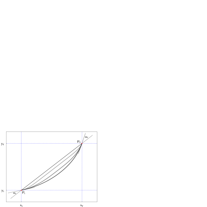
$x$

FIG. 1.: Different “Smooth Connection Functions” that connect the initial point $P_{i}:(x_{i},y_{i})$ with the final point $P_{f}:(x_{f},y_{f})$. At $P_{i}$ and $P_{f}$ the curves are tangent to the associated rays (dashed) which are specified by their inclination angles, $\alpha_{i}$ and $\alpha_{f}$, with respect to the vector pointing from $P_{i}$ to $P_{f}$. The light-gray curve (resulting from $\nu=1.2$) is the shortest, but has the strongest curvature. Conversely, the dark-grey curve ($\nu=20$) is the longest, but almost corresponds to an arc of a circle with minimal curvature. The intermediate grey curve ($\nu=2$) presents a more balanced compromise between minimal length and curvature.

$y(x)$

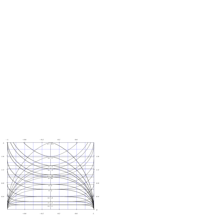
$x$

FIG. 2.: Standard smooth connection functions for various $\nu$. The two branches are monotonic and we have chosen the constants of integration such that they can be obtained from each other by a reflection with respect to the $y$-axis. Each SCF changes the sign of its curvature at $x=0$. For large $|\nu|$ the SCF is very close to the arc of a circle. The curves for $\nu>1$ are below the curve corresponding to $|\nu|\to\infty$. These curves become “flatter” and thus shorter for smaller values of $\nu$. They approach $x=0$ with a vanishing slope and their curvature radius diverges at $x=0$. The closer $\nu$ is to unity the sooner the curve approaches the value $y(0)$ when $x\to 0$. The curves for $\nu<0$ all reside above the curve corresponding to $|\nu|\to\infty$. For these curves both the slope $q(x)$ and the curvature radius $r(x)$ vanish at $x=0$.

$y(x)$

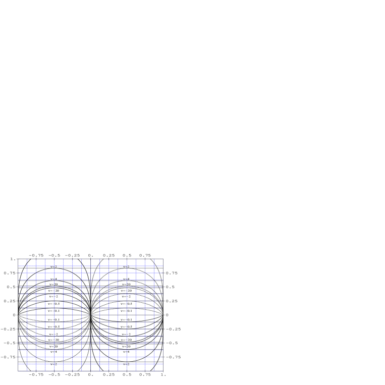
$x$

FIG. 3.: Extended standard smooth connection functions for various $\nu$. These functions are obtained from the SCFs of Fig. 2 by exchanging the coordinates $x$ and $y$. All curves have been rescaled such that they are defined in the interval $-1<x<1$. The interval $-1/2<x<1/2$ corresponds to the SCFs of Fig. 2. The continuations beyond $x=\pm 1/2$ use a segment of the other branch, which is attached to the centerpiece such that the curvature radius is continuous at $x=\pm 1/2$.

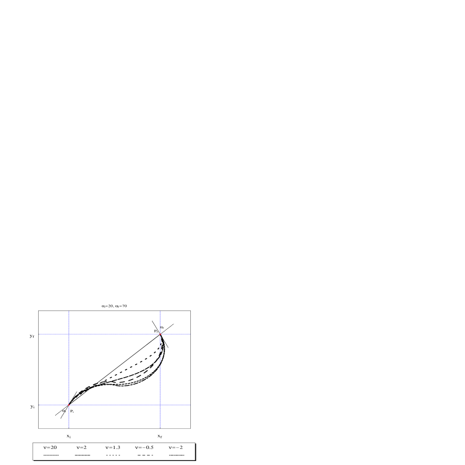
FIG. 4.: Example for a specific set of smooth connection functions that all satisfy the same boundary conditions. Each curve corresponds to a different $\nu$ as indicated in the legend. All the solutions consists of a segment of an extended standard smooth connection function that can be viewed as a template which may be rotated, translated and scaled in order to fit the boundary conditions. This example corresponds to $\alpha_{i}=20^{\circ}$ and $\alpha_{f}=70^{\circ}$.

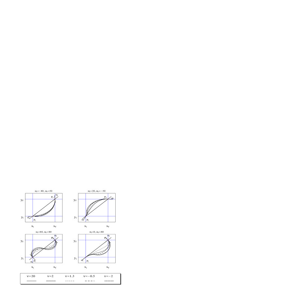
FIG. 5.: Examples for solving specific choices of $(\alpha_{i},\alpha_{f})$ with the (extended) standard SCFs. Each plot corresponds to a particular choice of $(\alpha_{i},\alpha_{f})$ and shows the behavior of the solution for five different values of $\nu$ as indicated in the legend.