Dark Area Theorem

Abstract

We report the discovery of a “dark area theorem,” a new quantum optical relation for propagation of unmatched pulses in thick three-level $\Lambda$-type media. We define dark area and derive the dark area theorem for a coherently prepared and inhomogeneously broadened lambda medium. We also obtain the first equation for the spatial evolution of the dark state amplitude prior to pulse-matching.

Many advances have been made recently in controlling quantum systems with a pair of near-resonant optical pulses under conditions of relatively long-preserved two-photon coherence among three quantum states. Key parameters being controlled include laser pulse intensity, frequency, duration, shape, timing and detuning. Well-known techniques and phenomena such as Rabi splitting [1], spectroscopic dark-states [2], pulse matching [3], and anti-intuitive excitation [4] have been exploited, with consequences including EIT (electromagnetically induced transparency [5]), LWI (lasing without inversion [6]), state-selective molecular excitation (STIRAP [7]), and demonstrations of slow light [8] and fast light [9], to mention only a few prominent examples.

However, in practically every instance a strong field is used to control a near-resonant medium so that a weak field can penetrate or amplify or excite transitions in a way normally forbidden. These are thin absorber applications, in the sense that the strong field’s evolution in the medium is ignored.

The understanding of pulse evolution in two-level media is much more complete. The McCall-Hahn Area Theorem [10] is available to provide a unifying picture of the way the medium acts back self-consistently. Even in situations where coherence is not complete, the two-level Area Theorem is a guide to the key role of self-consistent back action, and may suggest inverse applications in which the medium controls the field [11], i.e. thick absorber applications.

In the present note we report the discovery of a new nonlinear propagation law for unmatched pulses in a three-level medium. This new propagation law, which is appropriately labelled a Dark Area Theorem, takes the form:

$${\partial\theta_{D}\over\partial\zeta}=-{\alpha+\alpha^{\prime}\over 4}\sin(\theta_{D}+\phi)+{\alpha-\alpha^{\prime}\over 4}(\sin\theta_{D}+\sin\phi),$$ (1)

where the constant $\phi$ and the “dark area” $\theta_{D}$ are defined below. Here $\alpha$ and $\alpha^{\prime}$ are the conventional Beer’s Law absorption coefficients for the two transitions shown in Fig.  1(a).

The fundamental equations, from which the dark area theorem is derived, are familiar. For the physical pulses we have:

$${\partial\over\partial\zeta}\Omega_{g}=i\mu\langle\,ag^{*}\rangle\,,$$ (2)

$${\partial\over\partial\zeta}\Omega_{g^{\prime}}=i\mu^{\prime}\langle\,ag^{\prime*}\rangle\,,$$ (3)

where the notation is indicated in Fig. 1(a). The $\Omega$’s are the two Rabi frequencies of the (assumed unchirped) fields: $\Omega_{g}\equiv 2d_{g}{\cal E}_{g}/\hbar$, etc. The angular brackets are defined by $\langle(\dots)\rangle\equiv\int F(\Delta)(\dots)d\Delta$, which is an average over detunings arising from inhomogeneous broadening, where $F$ is a normalized distribution, taken symmetric and Gaussian in the examples calculated below, with $F_{0}$ setting the time scale for inhomogeneous relaxation. We take the same $F$ for the two transitions. The $\mu$ parameters are related to the $\alpha$’s in the standard way for inhomogeneously broadened media: $\alpha=\pi\mu F_{0}$, and $\alpha^{\prime}=\pi\mu^{\prime}F_{0}$, and we do not assume $\mu=\mu^{\prime}$. Finally, we have defined local-time coordinates $\tau$ and $\zeta$ in the frame propagating with velocity $c$ in the medium: $c\tau\equiv ct-z$ and $\zeta\equiv z$.

In addition to the two field equations there are three equations for the atomic amplitudes $g$, $g^{\prime}$ and $a$. We prefer to write these equations in the dressed “bright-dark” basis sketched in Fig. 1(b):

$$i{\partial\over\partial\tau}D=-{1\over 2}\Omega_{D}^{*}\,B\,,$$ (4)

$$i{\partial\over\partial\tau}B=-{1\over 2}\Omega_{B}\,a\,-{1\over 2}\Omega_{D}\,D\,$$ (5)

$$i{\partial\over\partial\tau}a=(\Delta-i\gamma)a-{1\over 2}\Omega_{B}~{}B,$$ (6)

where we have defined the bright Rabi frequency as $\Omega_{B}\equiv\sqrt{\Omega_{g}^{2}+\Omega_{g^{\prime}}^{2}}$, and the dark Rabi frequency via the Fleischhauer-Manka relation [12]: $\Omega_{D}=-i(\dot{\Omega}_{g}\Omega_{g^{\prime}}-\dot{\Omega}_{g^{\prime}}\Omega_{g})/\Omega_{B}^{2}$. In these equations and throughout the paper the symbols $B$ and $D$ denote the bright and dark state amplitudes, which are related by a well-known field-dependent dressing rotation [13] in $g$ - $g^{\prime}$ space:

$$\left[\begin{array}[]{c}B\\ D\\ \end{array}\right]=\left[\begin{array}[]{cc}\cos\theta/2&\sin\theta/2\\ -\sin\theta/2&\cos\theta/2\end{array}\right]\left[\begin{array}[]{c}g\\ g^{\prime}\\ \end{array}\right],$$ (7)

where $\cos\theta/2=\Omega_{g}/\Omega_{B}$ and $\sin\theta/2=\Omega_{g^{\prime}}/\Omega_{B}$.

However, we have discovered that the $\pm 2n\pi$ ambiguity of this definition of $\theta$ has physical meaning, and that the meaning is related to the spatial evolution of $\theta$. This is a double surprise - that the ambiguity is physical and that the dressing angle should be treated as a propagation variable, actually as an “area” corresponding to the dark Rabi frequency:

$$\theta(\zeta,\tau)\equiv i\int_{-\infty}^{\tau}\Omega_{D}(\zeta,\tau^{\prime})d\tau^{\prime}+\theta(\zeta,-\infty)\,,$$ (8)

where $\tan{1\over 2}\theta(\zeta,-\infty)\equiv\Omega_{g^{\prime}}(\zeta,-\infty)/\Omega_{g}(\zeta,-\infty)$. Now we explain these remarks by examining the previously unexplored spatial evolution of $\theta$.

The first Dark Area propagation equation is:

$${\partial\theta\over\partial\zeta}={2i\over\Omega_{B}}\Big{(}\mu_{+}\langle aD^{*}\rangle-\mu_{-}\langle aB^{*}\rangle\Big{)}\,,$$ (9)

where the coefficients are $\theta$-dependent and defined as $\mu_{+}\equiv{1\over 2}(\mu+\mu^{\prime})+{1\over 2}(\mu^{\prime}-\mu)\cos\theta$ and $\mu_{-}\equiv{1\over 2}(\mu-\mu^{\prime})\sin\theta$. This equation is derived from the definition of dark area and equations (2) and (3), and with it we obtain the key to the propagation regime. An expression for $\langle aD^{*}\rangle$ and $\langle aB^{*}\rangle$ can be obtained in two steps, first by formal integration of the $a$ equation up to a time $T$ following the passage of the pulses, to obtain

$$a(T;\Delta)={i\over 2}\int_{-\infty}^{T}e^{-(\gamma+i\Delta)(T-\tau)}\Big{(}\Omega_{B}~{}B\Big{)}d\tau,$$ (10)

and second by substituting this integral into the right side of (9), where the resulting double integrals (over $\tau$ and $\Delta$) can be evaluated [14]. This is done in the regime of rapid inhomogeneous relaxation, in which $F_{0}$ is a shorter time than the pulse durations or the medium’s homogeneous lifetimes, and we obtain at time $T$: $i\langle aD^{*}\rangle\approx-{\pi\over 2}F_{0}\Omega_{B}D_{0}B_{0}$ and $i\langle aB^{*}\rangle\approx-{\pi\over 2}F_{0}\Omega_{B}B_{0}^{2}$. The subscript $0$ here denotes $\Delta=0$.

Now we restrict attention to the case $\mu=\mu^{\prime}$ for simplicity in describing the developments, in which case the central propagation equation (9) reduces to:

$${\partial\theta_{D}\over\partial\zeta}={2i\mu\over\Omega_{B}}\langle aD^{*}\rangle=-\alpha D_{0}B_{0},$$ (11)

where $\theta_{D}$ is the total dark area, i.e., $\theta_{D}=\theta(\zeta,\tau>T)$. Within the $\tau>T$ regime we apply the solutions for $B$ and $D$ that are compatible with the asymptotic preparation of the medium, namely $B=\sin\frac{1}{2}\;(\theta_{D}+\phi)$ and $D=\cos\frac{1}{2}(\theta_{D}+\phi)$, where $\tan(\phi/2)=g/g^{\prime}$ taken at $\tau\to-\infty$. This converts (11) directly into the Dark Area Theorem:

$${\partial\theta_{D}\over\partial\zeta}=-{\alpha\over 2}\sin(\theta_{D}+\phi),$$ (12)

which is easily seen to be the reduced form of (1) when $\alpha=\alpha^{\prime}$. The more general equation (1) can be derived in the same way, simply by retaining $\alpha\neq\alpha^{\prime}$ throughout. The Dark Area theorem makes asymptotic predictions for the pulses, and assigns distinct physical content to each of the branches of its solution shown in Fig. 2.

As in the two-level case, the three-level area theorem does not predict pulse shapes, and an infinite variety of shapes can be asymptotically stable. In Fig. 3 we show the evolution of two initially unmatched and temporally offset pulses, with initial areas $1.5\pi$ and $4.8\pi$. Propagation over 20 Beer’s lengths shows highly non-trivial shifting and reshaping. In addition one can check that the final matched pulses conform to the dark area theorem’s asymptotic rule: their amplitude ratio is given by $\tan(\phi/2)$.

A further surprise arising from the use of the dressing angle as a propagation variable is that the spatial behavior of the bright and dark amplitudes is already specified by the dressing transformation itself. In the $\tau>T>F_{0}$ regime, where the space-time behavior of $B$ and $D$ is a self-consistent reponse to the pulses, we can write $\partial B/\partial\zeta=(\partial B/\partial\theta_{D})(\partial\theta_{D}/\partial\zeta)$, and a similar equation for $D$ . With the aid of (11), we can thereby obtain a new equation for $D^{2}$ alone: $\partial D^{2}/\partial\zeta=\alpha D^{2}(1-D^{2})$, with the elementary solution:

$$\ln{D^{2}(1-D_{in}^{2})\over(1-D^{2})D_{in}^{2}}=\alpha(\zeta-\zeta_{in}),$$ (13)

where $D_{in}$ here means the value of $D$ at the arbitrary position of incidence $\zeta_{in}$. The new $D^{2}$ equation itself already shows that the alternate solution $D=0$ is not stable, which is exactly the conclusion reached in our earlier numerical study of the distinction between $SIT$-type and $EIT$-type propagation [15].

More important, the analytic solution given here also provides the first compact predictive expression [16] for spatial evolution of the dark state toward matched pulses, and confirms what has been known empirically, that the real pulses finally must become matched, which is the same as the limit $D^{2}\to 1$. The straight lines of data points given in the inset in Fig. 4 show the agreement between a completely numerical solution obtained from the original equation set (2) - (6) and the simple expression (13) predicted by dark area theory. The two different lines of points emphasize that for different times $\tau/T^{*}$ in the pulse the spatial evolution of $|D|^{2}$ will attain the predicted asymptotic straight-line form more or less quickly.

To summarize, we have presented the explicit form of an area theorem that is, to the best of our knowledge, the first to be found for propagation in thick three-level media. The most important ingredient of the derivation was the discovery that $\theta_{D}$, twice the dark-state dressing angle, is the key propagation variable for physical pulses in coherently prepared three-level media [17]. We have demonstrated that, in the domain of rapid inhomogeneous relaxation, approximate expressions for the response of the medium can be found, and that they lead directly to compact expressions for the spatial evolution of bright and dark state amplitudes, as in eqn. (13), which were previously unknown. Numerical solutions show that these simple expressions are highly accurate.

We expect applications of the dark area theorem to be numerous and interesting. One can show that the singular points of both $\tan\theta_{D}$ and $\cot\theta_{D}$ determine the number of zero-crossings of the physical pulse envelopes $\Omega_{g}$ and $\Omega_{g^{\prime}}$, such as the two that appear spontaneously in Fig. 3 around $\alpha L=$ 5 and 10. Such zero-crossings appear closely related to phase jumps previously observed in Raman solitons [18]. The inclusion of inhomogeneous broadening makes the dark area theorem capable of addressing three-level echo effects [19]. Application of the singularity rules mentioned above will lead to non-trivial analogs of the McCall-Hahn rule for split-up of $2n\pi$ pulses. In conclusion, we mention again that the full expression of the theorem in eqn. (1) allows $\mu\neq\mu^{\prime}$. A detailed examination of (1) must be given elsewhere [20], along with the spatial development of the bright field $\Omega_{B}$ and other elements missing here for lack of space.

Acknowledgement: Research partially supported by NSF grants PHY94-15583 and PHY00-72359, and the programme QUIBITS of the European Commission.

Figure Captions

Fig. 1
a) Excitation of the bare-state atom by two pulsed fields, denoted by their Rabi frequencies $\Omega_{g}$ and $\Omega_{g^{\prime}}$, and b) excitation of the counterpart dressed-state atom by bright and dark fields, as defined in the text below eqn. (6).

Fig. 2
Evolution of the dark area $\theta_{D}$ with distance, as predicted by eqn. (1). Asymptotes are determined by $\theta_{D}+\phi=2n\pi$ and $\tan(\theta_{D}/2)\tan(\phi/2)=\alpha/\alpha^{\prime}$. The values used here are $\phi=2\pi/3$ and $\alpha^{\prime}=4\alpha$.

Fig. 3
Spatial snapshots of the evolution of two initially unmatched pulses with areas $1.5\pi$ and $4.8\pi$, through 20 Beer’s lengths of a $\Lambda$ medium with $\phi=2\pi/3$, obtained by exact numerical solution of eqns. (2)-(6), as a test of eqn. (12). The inhomogeneous detuning distribution $F(\Delta)$ is taken Gaussian, and local time is shown in units of $T^{*}=\sqrt{2\pi}F_{0}$. At $\alpha\zeta=20$ the pulses are almost matched, with $\Omega_{g^{\prime}}/\Omega_{g}\approx 1.6$, in good agreement with the final amplitude ratio predicted by the branch value of $\theta_{D}$, i.e., $\tan(2\pi-\phi)=\tan(4\pi/3)=\sqrt{3}$.

Fig. 4
Dark state population as a function of time is shown for five different depths of propagation of the same pulses shown in Fig. 3. Evolution to $|D|^{2}=1$ is evident. The specific prediction of eqn. (13) is also checked by computing $|D(\zeta,\tau)|^{2}$ for these pulses over 8 equal intervals at $\alpha\zeta=$ 0, 2.5, 5.0, …, 20.0 at both times $\tau/T^{*}=$ 15 and 30, indicated by vertical dashed lines in the right-hand half. The two sets of straight-line data with approximately unit slope shown in the inset provide excellent confirmation of the dark area theory.

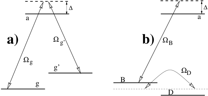
FIG. 1.: J.H. Eberly and V.V. Kozlov, “Dark Area Theorem”

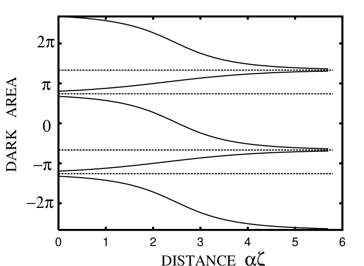
FIG. 2.: J.H. Eberly and V.V. Kozlov, “Dark Area Theorem”

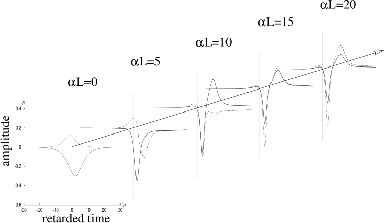
FIG. 3.: J.H. Eberly and V.V. Kozlov, “Dark Area Theorem”

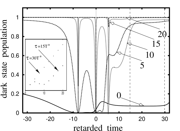
FIG. 4.: J.H. Eberly and V.V. Kozlov, “Dark Area Theorem”

REFERENCES

- [1] For example, see S.H. Autler and C.H. Townes, Phys. Rev. 100, 703 (1955), and B.R. Mollow, Phys. Rev. 188, 1969 (1969).
- [2] See G. Alzetta, A. Gozzini, L. Moi, and G. Orriols, N. Cim. B 36, 5 (1976); E. Arimondo and G. Orriols, Lett. N. Cim. 17, 333 (1976); and R. M. Whitley and C. R. Stroud, Jr., Phys. Rev. A 14, 1498 (1976).
- [3] For matched pulses in multi-level situations see Sec. II of R.J. Cook and B.W. Shore, Phys. Rev. A 20, 539 (1979), and F.T. Hioe and J.H. Eberly, Phys. Rev. A 25, 2168 (1982). See also S.E. Harris, Phys. Rev. Lett. 72, 52 (1994) and J.H. Eberly, M.L. Pons and H.R. Haq, Phys. Rev. Lett. 72, 56 (1994).
- [4] J. Oreg, F. T. Hioe, and J. H. Eberly, Phys. Rev. A 29, 690 (1984).
- [5] S. E. Harris, Physics Today 50, 36 (1997). See also K.-J. Boller, A. Imamoglu, and S. E. Harris, Phys. Rev. Lett. 66, 2593 (1991); and S. E. Harris, ibid 70, 552 (1993).
- [6] O. A. Kocharovskaya and Ya. I. Khanin, Pis’ma Zh. Eksp. Teor. Fiz. 48, 581 (1988); S. E. Harris, Phys. Rev. Lett. 62, 1033 (1989); and M. O. Scully, S.-Y. Zhu, and A. Gavrielides, ibid 62, 2813 (1989).
- [7] U. Gaubatz, P. Rudecki, M. Becker, S. Schiemann, M. Külz and K. Bergmann, Chem. Phys. Lett. 149, 463 (1988).
- [8] See L.V. Hau, S.E. Harris, Z. Dutton, and C.H. Behroozi, Nature 397, 594 (1999); M.M. Kash, V.A. Sautenkov, A.S. Zibrov, L. Hollberg, G.R. Welch, M.D. Lukin, Y. Rostovtsev, E.S. Fry, and M.O. Scully, Phys. Rev. Lett. 82, 5229 (1999); D. Budker, D.F. Kimball, S.M. Rochester, and Y.Y. Yashchuk, ibid 83, 1767 (1999).
- [9] See R. Y. Chiao, Phys. Rev. A 48, R34 (1993); and L. J. Wang, A. Kuzmich and A. Dogariu, Nature 406, 277 (2000).
- [10] S. L. McCall and E. L. Hahn, Phys. Rev. Lett. 18, 908 (1967), and Phys. Rev. 183, 457 (1969).
- [11] For example, photon echo generation as in E.L. Hahn, N.S. Shiren and S.L. McCall, Physics Lett. 37A, 265 (1971), or pulse steepening as in H.M. Gibbs and R.E. Slusher, Appl. Phys. Lett. 18, 505 (1971).
- [12] M. Fleischhauer and A.S. Manka, Phys. Rev. A 54, 794 (1996).
- [13] J.R. Kuklinski, U. Gaubatz, F.T. Hioe, and K. Bergmann, Phys. Rev. A 40, 6741 (1989). Here is used for what we label , but its role in propagation is not considered.
- [14] J.H. Eberly, Optics Expr. 2, 173 (1998).
- [15] V. V. Kozlov and J. H. Eberly, Optics Comm. 179, 85 (2000).
- [16] Predictive expressions of three-level SIT type are well-known, beginning with M.J. Konopnicki and J.H. Eberly, Phys. Rev. A 24, 2567 (1981), but few examples in EIT-type domains are known: for an overview, see [12] above. None of these examples identifies dark area, or recognizes the state dressing angle as a propagation variable.
- [17] Recall that in dressed-state treatments of two-level interactions the dressing angle is half the Bloch-sphere angle , which is of course also the two-level area.
- [18] See, for example, K. Drühl, R. G. Wenzel and J. L. Carlsten, Phys. Rev. Lett. 51, 1171 (1983); and D. C. MacPherson, R. C. Swanson, and J. L. Carlsten, Phys. Rev. A 40, 6745 (1989).
- [19] S.R. Hartmann, IEEE J. Quantum Elect. QE-4, 802 (1968).
- [20] V. V. Kozlov and J. H. Eberly, in preparation.