Fluctuation Analysis of Human Electroencephalogram

Abstract

The scaling behaviors of the human electroencephalogram (EEG) time series are studied using detrended fluctuation analysis. Two scaling regions are found in nearly every channel for all subjects examined. The scatter plot of the scaling exponents for all channels (up to 129) reveals the complicated structure of a subject’s brain activity. Moment analyses are performed to extract the gross features of all the scaling exponents, and another universal scaling behavior is identified. A one-parameter description is found to characterize the fluctuation properties of the nonlinear behaviors of the brain dynamics.

PACS numbers: 05.45.Tp, 87.19.La, 87.90.+y

In the study of electrical activities of the brain recorded by electroencephalogram (EEG) various methods have been used to extract different aspects of the neuronal dynamics from the scalp potentials. They range from the traditional linear analysis that involves frequency decomposition, topographic mapping, etc. [1, 2], to time-frequency analysis that uses wavelet transform[3], to nonlinear analysis that is particularly suitable for learning about the chaotic behavior of the brain[4] or for quantifying physiological conditions in nonlinear-dynamics terms [5, 6]. In this paper we discuss the scaling behavior of the fluctuations in EEG in nonlinear analysis and show the existence of new features in brain dynamics hitherto unrecognized. Moreover, we propose a global measure of the spatio-temporal signals that has potential utility in clinical and cognitive diagnostics.

Apart from being more suitable to analyze non-stationary time series, the study of scaling behavior emphasizes the relationship across time scales and provides a different description of the time series than the conventional Fourier power spectrum. Conveniently it also liberates our result from the dependence on the magnitude of the voltage recorded by each probe. We aim to find what is universal among all channels as well as what varies among them. The former is obviously important by virtue of its universality for a given subject; how that universal quantity varies from subject to subject would clearly be interesting. The latter, which is a measure that varies from channel to channel, is perhaps even more interesting, since that quantity has brain anatomical correlates once the scalp potentials have been deconvolved to the cortical surface.

Our procedure is to focus initially on one channel at a time. Thus it is a study of the local temporal behavior and the determination of a few parameters (scaling exponents) that effectively summarize the fluctuation properties of the time series. The second phase of our procedure is to describe the global behavior of all channels and to arrive at one number that summarizes the variability of these temporal measures across the entire scalp surface. This dramatic data reduction necessarily trades detail for succinctness, but such reduction is exactly what is needed to allow easy discrimination between brain states.

The specific method we use in the first phase is detrended fluctuation analysis (DFA). This analysis is not new. It was proposed for the investigation of correlation properties in non-stationary time series and applied to the studies of heartbeat [7] and DNA nucleotides [8]. It has also been applied to EEG[9], but with somewhat different emphases than those presented here. Since the analysis considers only the fluctuations from the local linear trends, it is insensitive to spurious correlations introduced by non-stationary external trends. By examining the scaling behavior one can learn about the nature of short-range and long-range correlations, which are a salient aspect of the brain dynamics from the viewpoint of complex systems theory.

Let an EEG time series be denoted by $y(t)$, where $t$ is discrete time ranging from 1 to $T$. Divide the entire range of $t$ to be investigated into $B$ equal bins, discarding any remainder, so that each bin has $k={\rm floor}(T/B)$ time points. Within each bin, labeled $b\ (b=1,\cdots,B)$, perform a least-square fit of $y(t)$ by a straight line, $\overline{y}_{b}(t)$, i.e., $\overline{y}_{b}(t)=$ Linear-fit$[y(t)]$ for $(b-1)k<t\leq bk$. That is the semi-local trend for the $\it b$th bin. Combine $\overline{y}_{b}(t)$ for all $B$ bins and denote the $B$ straight segments by

$$\overline{y}(k,t)=\sum_{b=1}^{B}\overline{y}_{b}(t)\,\theta(t-(b-1)k)\,\theta(bk-t)$$ (1)

for $1\leq t\leq kB$. Define

$$F^{2}(k)={1\over{kB}}\sum_{t=1}^{kB}\ [\,y(t)-\overline{y}(k,t)\,]^{2}.$$ (2)

$F(k)$ is then the RMS fluctuation from the semi-local trends in $B$ bins each having $k$ time points, and is also a measure of the fluctuation in each bin averaged over $B$ bins. The study of the dependence of $F(k)$ on the bin size $k$ is the essence of DFA [7, 8]. If it is a power-law behavior

$$F(k)\propto k^{\alpha},$$ (3)

then the scaling exponent $\alpha$ is an indicator of the power-law correlations of the fluctuations in EEG, and is independent of the magnitude of $y(t)$ or any spurious trend externally introduced.

Resting EEG data were collected for six subjects using a 128-channel commercial EEG system, with scalp-electrode impedences ranging from 10 to 40 k$\Omega$. The acquisition rate is 250 points/sec with hardware filtering set between 0.1 and 100 Hz. After acquisition, $T\approx 10$s lengths of simultaneous time series in all channels are chosen, free of artifacts such as eye blink and head movements. At each time point, the data are re-referenced to the average over all electrodes. This approximates the potentials relative to infinity, and provides a more interpretable measure of local brain activity[2]. We investigate the range of $k$ from 3 to 500 in approximately equal steps of $\ln k$.

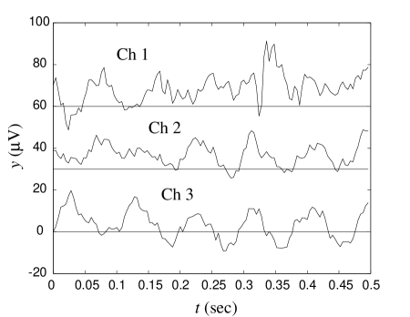
FIG. 1.: A sample of EEG time series in three channels. The vertical scales of Ch 1 and Ch 2 are shifted upward by 60 and 30 $\mu$V, respectively.

In Fig. 1 we show three typical time series $y(t)$ in three widely separated channels for subject A, labeled 1-3, for brevity. While it is clear that both channels 2 and 3 have substantial 10 Hz oscillations after 0.2 s, it is much less apparent that there exist any scaling behaviors in all three channels. The corresponding values of $F(k)$ are shown in the log-log plot in Fig. 2. Evidently, the striking feature is that there are two scaling regions with a discernible bend when the two slopes in the two regions are distinctly different. With rare exceptions this feature is found in all channels for all subjects. Admittedly, the extents of the scaling regions are not wide, so the behavior does not meet the qualification for scaling in large critical systems or in fractal geometrical objects. However, since the behavior is so universal across channels and subjects, it is a feature of EEG that conveys an important property of the brain activity and should not be ignored.

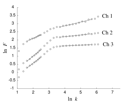
FIG. 2.: $F(k)$ vs $k$ for the three channels in Fig. 1. The vertical scales of Ch 1 and Ch 2 are shifted upwards by 1.0 and 0.5 units, respectively.

To quantify the scaling behavior, we perform a linear fit in Region I for $1<\ln k<2.5$ and denote the slope by $\alpha_{1}$, and similarly in Region II for $3.5<\ln k<5.75$ with slope denoted by $\alpha_{2}$. Knowing the two straight lines in each channel allows us to determine the location of their intercept, $\ln\kappa$, which we define as the position of the bend in $\ln k$. We find that, whereas $\alpha_{1}$ and $\alpha_{2}$ can fluctuate widely from channel to channel, $\kappa$ is limited to a narrow range in most subjects. The average values of $\ln\kappa$ for the six subjects are 3.45, 3.66, 3.10, 2.92, 2.60, and 3.12.

Since the only quantity in our analysis that has a scale is $k$, the size of the bin on the time axis in which fluctuations from the semi-local trend are calculated, the specific scale $\kappa$ must correspond roughly to a particular frequency $f$. If the data acquisition rate is denoted by $r$, then $f=r/\kappa$. For $r=250$ points/sec, and $\ln\kappa=3.45$, we get $f=7.94$ Hz. That is near the midpoint separating the traditional $\alpha$ (8-13 Hz) and $\theta$ (5-8 Hz) EEG frequency bands. Region I is then at higher frequencies, Region II lower. Thus in this nonlinear analysis we have found the existence of a specific frequency in every channel that separates different scaling behaviors. A change in scaling exponent in physical systems is often attributable to distinct dynamical processes underlying the generation of the time series. An interesting question is how this finding relates to EEG neurophysiology.

We now exhibit the values of $\alpha_{1}$ and $\alpha_{2}$ of all channels for subject A in a scatter plot in Fig. 3. They vary in the ranges: $0.19<\alpha_{1}<1.44$ and $0.018<\alpha_{2}<0.489$. Whereas $\alpha_{1}$ is widely distributed, $\alpha_{2}$ is sharply peaked at 0.1 and has a long tail. The value of $\alpha=0.5$ corresponds to random walk with no correlation among the various time points. For $\alpha\neq 0.5$ there are correlations: Region I corresponds to short-range correlation, Region II long-range, with $\kappa$ giving a quantitative demarkation between the two. It is natural to conjecture that high deviations of the $\alpha$ values from the average could be caused by pathological conditions. Since the two scaling regions have corresponding frequency bands, one would likely want to focus on Region II to study brain states characterized by marked $\delta$ (1-4 Hz) and $\theta$ (5-8 Hz) activity. Sleep and cerebral ischemic stroke are two such examples.

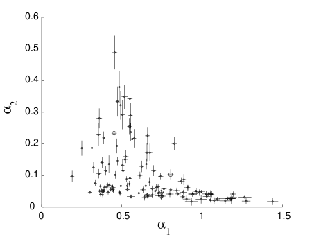
FIG. 3.: Scatter plot of $\alpha_{2}$ vs $\alpha_{1}$ for subject A. The three channels exhibited in Figs. 1 and 2 are shown as big circles.

So far our consideration has focused on the temporal properties of the time series in each channel. The scatter plot of $\alpha_{2}$ vs $\alpha_{1}$ provides a view of the complicated activities in all channels over the entire scalp. While the detailed spatial structure may be of interest for relating the values of $\alpha_{i}$ to brain anatomy, there is also a need for a general, overall description of all the pairs $\alpha_{i}$. A global measure for each subject could be of great use to specialists and non-specialists alike. To that end, we now consider the relationship among the $\alpha_{i}$ values, or more precisely, the fluctuation of $\alpha_{i}$.

Let $x$ be either $\alpha_{1}$ or $\alpha_{2}$, and $N$ be the total number of channels whose $\alpha_{i}$ values are under consideration. Since no value of $\alpha_{i}$ has been found to exceed 1.5 in the subjects we have examined, we consider the interval $0\leq x\leq 1.5$. Divide that interval into $M$ equal cells, which for definiteness we take to be $M=150$ here. Let the cells be labeled by $m=1,\cdots,M$, each having the size $\delta x=1.5/M$. Denote the number of channels whose $x$ values are in the $m$th cell by $n_{m}$. Define

$$P_{m}=n_{m}\,/\,N.$$ (4)

It is the fraction of channels whose $x$ values are in the range $(m-1)\,\delta x\leq x<m\,\delta x$. By definition, we have $\sum_{m=1}^{M}\,P_{m}=1$. In Fig. 4 we show as an illustration the two graphs of $P_{m}$ for subject A, three of whose EEG times series are shown in Fig. 1. The two graphs correspond to $\alpha_{1}$ and $\alpha_{2}$, and are, in essence, the projections of the scatter plot in Fig. 3 onto the $\alpha_{1}$ and $\alpha_{2}$ axes.

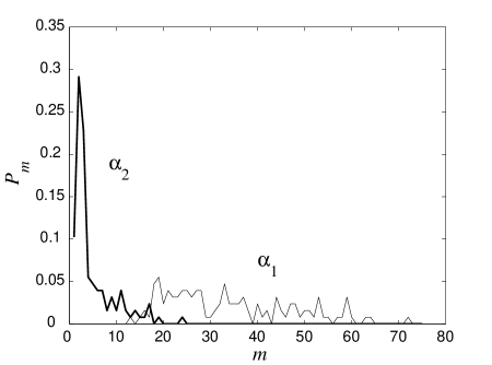
FIG. 4.: The distributions $P_{m}$ for $\alpha_{1}$ and $\alpha_{2}$ for subject A. The bin size in $\alpha$ for this plot is 0.02.

Instead of studying the complicated structures of the distributions $P_{m}$ themselves, it is more convenient to examine the moments of $P_{m}$. Thus we define the normalized moments

$$G_{q}=\sum_{m=1}^{M}\,m^{q}\,P_{m}\left/(\sum_{m=1}^{M}\,m\,P_{m})^{q},\right.$$ (5)

where $q$ is a positive integer, although it can be a continuous variable. Since $x$ can be either $\alpha_{1}$ or $\alpha_{2}$, we shall use $P_{m}^{(1)}$ and $P_{m}^{(2)}$ to denote the two distributions, and $G_{q}^{(1)}$ and $G_{q}^{(2)}$, respectively, for their moments. Since these moments are averages of $(m/\overline{m})^{q}$, where $\overline{m}$ is the average-$m$, they are not very sensitive to $\overline{m}$ itself. They contain the essence of the fluctuation properties of $\alpha_{1,2}$ in all channels.

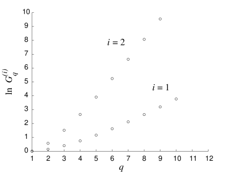
FIG. 5.: The $q$ dependence of $\ln G_{q}^{(i)}$ for subject A.

In principle, it is possible to examine also the moments for $q<0$, which would reveal the properties of $P_{m}$ at low values of $m$. However, the accuracy of our data is not too reliable for low-$k$ analysis, since the 60 Hz noise due to ambient electric and magnetic fields has not been cleanly filtered out. In this paper, therefore, we restrict our study to only the positive $q$ values. For high $q$, the large $m/\overline{m}$ parts of $P_{m}^{(1,2)}$ dominate $G_{q}^{(1,2)}$.

In Fig. 5 the $q$-dependences of $\ln G_{q}^{(1,2)}$ are shown for the distributions exhibited in Fig. 4 for $0\leq q\leq 10$. They appear to depend on $q$ quadratically. The relationship between $G_{q}^{(1)}$ and $G_{q}^{(2)}$ is, however, extremely simple, as can be shown by plotting them against each other in a log-log graph. In Fig. 6 we show the straightline behavior for three of the six subjects, all of whose EEG time series have been analyzed in the same method described here. Thus we can associate a slope $\eta$ to every subject, and conclude that there exists a universal scaling behavior

$$G_{q}^{(2)}\propto\left(\,G_{q}^{(1)}\,\right)^{\eta}.$$ (6)

This remarkable behavior is valid for all subjects examined, but the exponent $\eta$ varies from subject to subject. Thus we have discovered a measure that characterizes all the $\alpha_{i}$ values of a subject.

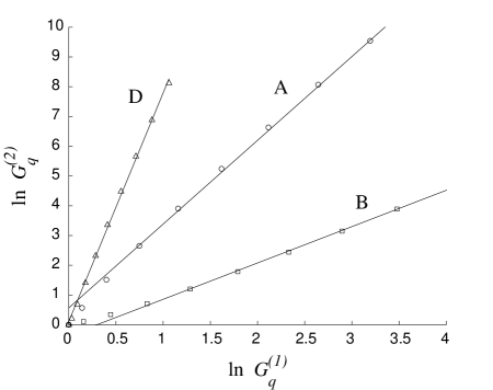
FIG. 6.: A log-log plot of $G_{q}^{(2)}$ vs $G_{q}^{(1)}$ for three subjects. The solid lines are linear fits of the large $q$ parts of the plots.

We label the six subjects whom we have examined as A-F. Their $\eta$ values are given below behind the subject labels.

A (2.82), B (1.22), C (1.74), D (7.68), E (6.39), F (3.29)

At this stage of our investigation we have not yet arrived at a point where we can give a definitive correlation between the values of $\eta$ and some specific aspect of the brain activity. It is, nevertheless, of interest to note that the subjects A-C were regarded as healthy control subjects, while D-F have each had recent encounter with ischemic stroke.

Before any tentative correlations may be inferred, we emphasize the need for caution since many factors were involved in data acquisition, e.g., varying degrees of awakeness of the subjects. Clinical and cognitive application is not the main object of this paper. However, the intriguing possibilities of the method presented here suggest extensive application of the analysis to many more subjects and for further investigation on what the scaling behaviors of the spatio-temporal EEG reveal. Such behaviors can undoubtedly be useful in guiding future theoretical development.

To summarize, we have studied the scaling properties of the fluctuations in the time series, and found a number of features previously unrecognized in power spectrum analysis. The characterization of the temporal behavior of each channel by just two parameters, $\alpha_{1}$ and $\alpha_{2}$, has led to the discovery of the $\eta$ exponent. Although $\eta$ is obtained by considering the global property of all channels, we envisage its extension to the study of local properties by the application of the moment analysis to partitioned regions of the scalp. Future possibilities of this approach to the investigation of EEG signals seem bountiful.

We are grateful to Dr. Phan Luu and Prof. Don Tucker for supplying the EEG data for our analysis. This work was supported, in part, by the U. S. Department of Energy under Grant No.  DE-FG03-96ER40972, and the National Institutes of Health under Grant No. R44-NS-38829.

REFERENCES

- [1] Electroencephalography: Basic Principles, Clinical Applications, and Related Fields, edited by E. Niedermeyer and F. H. Lopes da Silva (Urban and Schwarzenberg, Baltimore, 1987); ibid (Williams and Wilkins, Baltimore, 1998).
- [2] P. L. Nunez, Neocortical Dynamics and Human EEG Rythms (Oxford University Press, 1995).
- [3] S. Blanco, C. D’Attellis, S. Isaacson, O. A. Rosso, and R. Sirne, Phys. Rev. E 54, 6661 (1996); S. Blanco, A. Figliola, R. Quian Quiroga, O. A. Rosso, and E. Serrano, Phys. Rev. E 57, 932 (1998).
- [4] Chaos in Brain?, edited by K. Lehnertz, J. Arnhold, P. Grassberger and C. E. Elger (World Scientific, Singapore, 2000).
- [5] B. H. Jansen and M. E. Brandt, Nonlinear Dynamical Analysis of the EEG (World Scientific, Singapore, 1993).
- [6] K. Lehnertz and C. E. Elger, Phys. Rev. Lett. 80, 5019 (1998).
- [7] C.-K. Peng, S. Havlin, H. E. Stanley, and A. L. Goldberger, Chaos 5, 82 (1995).
- [8] C.-K. Peng, S. V. Buldyrev, S. Havlin, M. Simons, H. E. Stanley, and A. L. Goldberger, Phys. Rev. E 49, 1685 (1994).
- [9] Watters, P. A. Complexity International 5, 1 (1998).