STATIC AND DYNAMIC REGIMES OF ARBITRARY GAIN COMPENSATION SINGLE-MODE LASER DIODES

Abstract

We report on a methodology for the evaluation of the DC characteristics, small-signal frequency response and large-signal dynamic response of carrier and photon density responses in semiconductor laser diodes. A single mode laser is considered and described with a pair of rate equations containing a novel non-linear gain compensation term depending on a single parameter that can be chosen arbitrarily. This approach can be applied to any type of solid-state laser as long as it is described by a set of rate equations.

Keywords: Optoelectronic devices. Solid-state lasers. Dynamics.

I Introduction

Generally, lasers are described with a set of rate equations describing the generation-recombination of carriers or emission-absorption of photons. The equations are typically systems of first-order differential equations belonging to the population evolution type.

In this report we specialize to the simple case of single-mode laser diode where the system of equations reduces to two: one for the carrier population (density) and another for the photon population (density). We concentrate on the case the equations embody a novel non-linear gain compensation term that depends on a single parameter that can be chosen arbitrarily. The effect of this parameter is studied on the DC characteristics, small-signal frequency response and large-signal dynamic response of the laser.

The Single Mode (SM) laser diode rate equations are written as:

$$\frac{dN}{dt} = \frac{I}{qV}-\frac{N}{\tau_{n}}-g(N-N_{t})\frac{S}{{(1+\epsilon S)}^{b}}$$ (1)

$$\frac{dS}{dt} = \frac{\Gamma\beta N}{\tau_{n}}-\frac{S}{\tau_{ph}}+\Gamma g(N-N_{t})\frac{S}{{(1+\epsilon S)}^{b}}$$ (2)

$N$ represents the electron density ($N_{t}$ at transparency) and $S$ the photon density. $\tau_{n}$ is the electron spontaneous lifetime and $\tau_{ph}$ is the photon lifetime. $\beta$ is the fraction of spontaneous emission coupled to the lasing mode, $G$ the optical confinement factor, $g$ is the differential gain and $\epsilon$ is the gain compression parameter. $q$ is the electron charge, $V$ the volume of the active region and $I$ is the injection current which, in general, is a function of time.

The main novelty in these equations lie in the non-linear gain factor that has been traditionally modelled by the term $g(1-\epsilon S)$, $g/(1+\epsilon S)$ or even $g/\sqrt{(1+\epsilon S)}$ agrawal . In this study, this term is taken to an arbitrary power ning b in the interval [0,1.5]. In order to cover in the simulation the case $g(1-\epsilon S)$, we formally allocate b=-1 to this case. We analyse in this work the effects b has on the static, small- signal frequency response as well as the large-signal temporal variation of the carrier and photon densities.

This report is organized as follows: in section 2 we outline the evaluation of the Laser $S-I$ (photon density versus injection current) DC characteristics. In section 3, the small-signal frequency response is derived and in section 4, we illustrate the laser response to time-dependent injection currents and section 5 contains our conclusions.

II DC CHARACTERISTICS

The DC limit of the SM laser rate equations is given by:

$$0 = \frac{I}{qV}-\frac{N}{\tau_{n}}-g(N-N_{t})\frac{S}{{(1+\epsilon S)}^{b}}$$ (3)

$$0 = \frac{\Gamma\beta N}{\tau_{n}}-\frac{S}{\tau_{ph}}+\Gamma g(N-N_{t})\frac{S}{{(1+\epsilon S)}^{b}}$$ (4)

From (4) we extract the value of $(N-N_{t})$ as:

$$(N-N_{t})=\left[\frac{\frac{S}{\tau_{ph}}-\frac{\Gamma\beta N_{t}}{\tau_{n}}}{\Gamma g\frac{S}{{(1+\epsilon S)}^{b}}+\frac{\Gamma\beta}{\tau_{n}}}\right]$$ (5)

and substitute it in (3) relating $I$ to $S$ directly. This results in:

$$\frac{I}{qV}=\frac{N_{t}}{\tau_{n}}+\frac{(S-\Gamma\beta N_{t})(\frac{1}{\tau_{n}}+g\frac{S}{{(1+\epsilon S)}^{b}})}{\tau_{ph}[\Gamma g\frac{S}{{(1+\epsilon S)}^{b}}+\frac{\Gamma\beta}{\tau_{ph}}]}$$ (6)

This relation gives $I$ as a function of $S$. Generating a series of data values $(S,I)$ by varying $S$ and reverse writing them as $(I,S)$ will result in the $S-I$ DC characteristic.

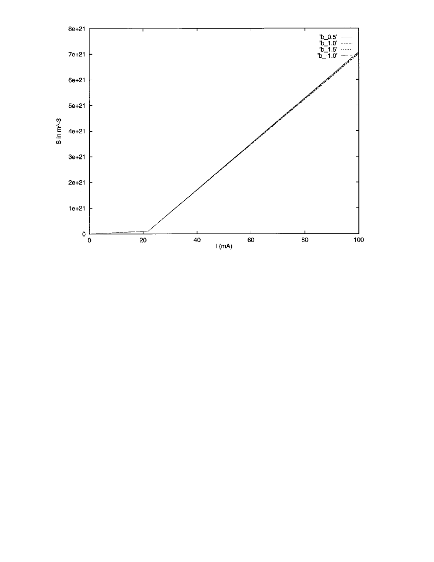
Figure 1: $S-I$ characteristics (Laser A) for various values of b: -1.0, 0.5, 1.0 and 1.5. The different values of b do not affect significantly the DC characteristics.

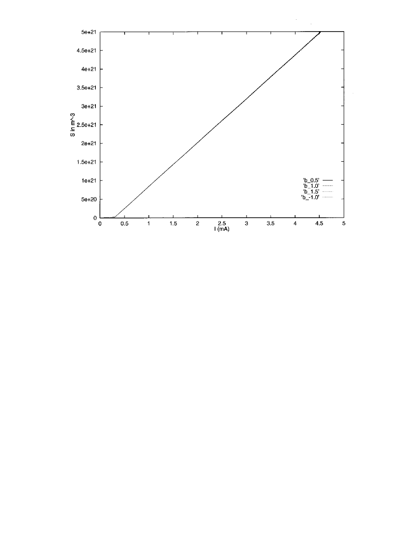
Figure 2: $S-I$ characteristics (Laser B) for various values of b: -1.0, 0.5, 1.0 and 1.5. The different values of b do not affect significantly the DC characteristics.

We consider two laser models A and B (Physical parameters given in Appendix A) and illustrate this procedure with the characteristics displayed in Figures 1 and 2 for different values of b. It appears from the figures that b does not affect significantly the DC characteristics in contrast with the frequency response and dynamic response as seen in the next sections.

III SMALL-SIGNAL FREQUENCY RESPONSE

In order to derive the small signal frequency response, we assume all quantities $I$, $N$ and $S$ are taken around some equilibrium values $I_{0}$, $N_{0}$ and $S_{0}$ and hence:

$$I=I_{0}+\delta I(t),N=N_{0}+\delta N(t),S=S_{0}+\delta S(t)$$ (7)

This means that equation (1) under variation (7) reads:

$$\frac{d\delta N}{dt}=\frac{\delta I}{qV}-\frac{\delta N}{\tau_{n}}-g\delta N\frac{S_{0}}{{(1+\epsilon S_{0})}^{b}}-g(N_{0}-N_{t})[\frac{1}{{(1+\epsilon S_{0})}^{b}}-\frac{\epsilon S_{0}b}{{(1+\epsilon S_{0})}^{b+1}}]\delta S\\$$ (8)

whereas (2) becomes:

$$\frac{d\delta S}{dt}=\frac{\Gamma\beta\delta N}{\tau_{n}}-\frac{\delta S}{\tau_{ph}}+\Gamma g\delta N\frac{S_{0}}{{(1+\epsilon S_{0})}^{b}}+\Gamma g(N_{0}-N_{t})[\frac{1}{{(1+\epsilon S_{0})}^{b}}-\frac{\epsilon S_{0}b}{{(1+\epsilon S_{0})}^{b+1}}]\delta S\\$$ (9)

In order to tackle the small-signal frequency response we switch to the time-harmonic case where the time derivatives are given by: $d\delta I/dt=j\omega\delta I,d\delta N/dt=j\omega\delta N,d\delta S/dt=j\omega\delta S$. This results in a system of equations relating the three variations $\delta I$, $\delta N$ and $\delta S$:

$$\delta N(j\omega+\frac{1}{\tau_{n}}+g\frac{S_{0}}{{(1+\epsilon S_{0})}^{b}})=\frac{\delta I}{qV}-g(N_{0}-N_{t})[\frac{1}{{(1+\epsilon S_{0})}^{b}}-\frac{\epsilon S_{0}b}{{(1+\epsilon S_{0})}^{b+1}}])\\$$ (10)

and:

$$\delta N(\frac{\Gamma\beta}{\tau_{n}}+g\frac{\Gamma S_{0}}{{(1+\epsilon S_{0})}^{b}})=\delta S(j\omega+\frac{1}{\tau_{ph}}-\Gamma g(N_{0}-N_{t})[\frac{1}{{(1+\epsilon S_{0})}^{b}}-\frac{\epsilon S_{0}b}{{(1+\epsilon S_{0})}^{b+1}}]\\$$ (11)

Taking the ratio of the above yields the small-signal frequency response:

$$\frac{\delta S}{\delta I}=\frac{1/E}{C+j\omega G-\omega^{2}}$$ (12)

where $E$, $G$ and $C$ are given by:

$$E=\frac{qV}{\left[\Gamma g\frac{S_{0}}{{(1+\epsilon S_{0})}^{b}}+\frac{\Gamma\beta}{\tau_{n}}\right]},$$ (13)

$$G=\frac{1}{\tau_{n}}+\frac{1}{\tau_{ph}}-\Gamma g(N_{0}-N_{t})[\frac{1+\epsilon S_{0}(1-b)}{{(1+\epsilon S_{0})}^{b+1}}]+\frac{gS_{0}}{{(1+\epsilon S_{0})}^{b}},$$ (14)

$$C=\frac{1}{\tau_{n}\tau_{ph}}-\frac{1}{\tau_{n}}\Gamma g(N_{0}-N_{t})(1-\beta)[\frac{1+\epsilon S_{0}(1-b)}{{(1+\epsilon S_{0})}^{b+1}}]+\frac{1}{\tau_{ph}}\frac{gS_{0}}{{(1+\epsilon S_{0})}^{b}}.$$ (15)

The standard normalised form ( 0 dB at 0 frequency) of the frequency response is taken as:

$$\widehat{\frac{\delta S}{\delta I}}=\frac{1}{1+j\omega G/C-\omega^{2}/C}$$ (16)

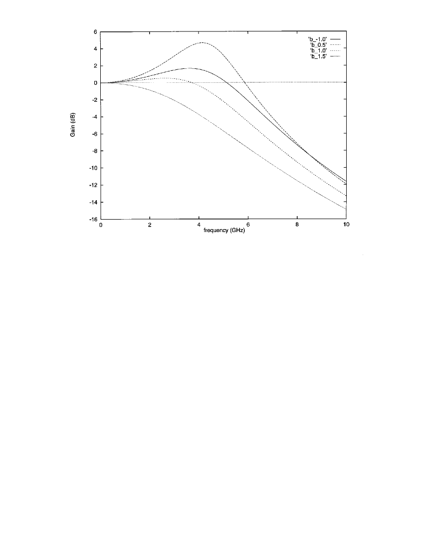
Figure 3: Small signal frequency response amplitude (Laser A) versus frequency for various values of b. From top to bottom, b is -1.0, 0.5, 1.0 and 1.5 respectively. The bias current is chosen as 40 mA.

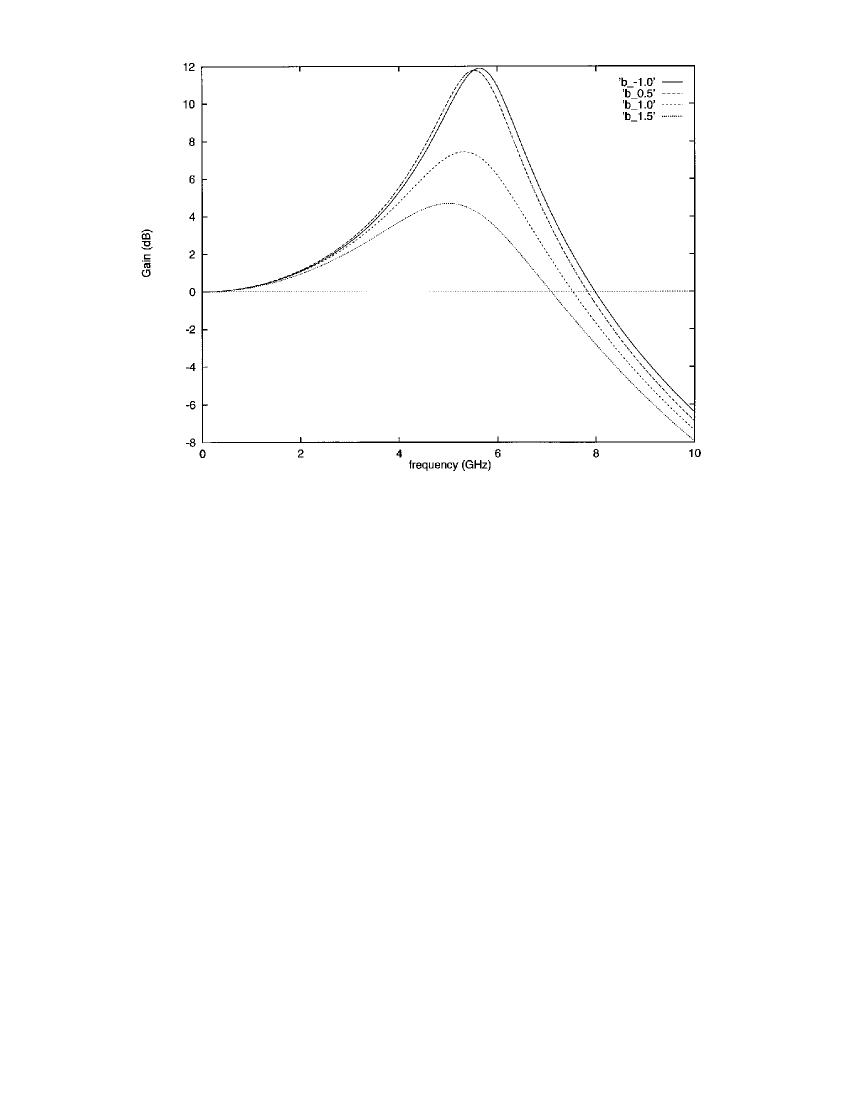
Figure 4: Small signal frequency response amplitude (Laser B) versus frequency for various values of b. From top to bottom, b is -1.0, 0.5, 1.0 and 1.5 respectively. The bias current is chosen as 1 mA.

It is displayed for laser A and B in Figures 3 and 4 for different values of b.

In sharp contrast with the DC case, the value of b, has a drastic effect on the frequency response as observed in the above figures. We differ from Way way in the frequency response due to a discrepancy in the estimation of the resonance frequency. Way defines the resonance frequency as (using our own notation and adapting it to Way’s way case):

$$f_{r}=\frac{1}{2\pi}\sqrt{(\frac{\Gamma N_{t}g\tau_{ph}+1}{\tau_{n}\tau_{ph}})}\sqrt{(I/I_{th}-1)}$$ (17)

where $I$ is the bias and $I_{th}$ is the threshold current. Our corresponding formula by inspection of (16) would be:

$$f_{r}=\frac{1}{2\pi}\sqrt{\frac{1}{\tau_{n}\tau_{ph}}-\frac{1}{\tau_{n}}\Gamma g(N_{0}-N_{t})(1-\beta)[\frac{1+\epsilon S_{0}(1-b)}{{(1+\epsilon S_{0})}^{b+1}}]+\frac{1}{\tau_{ph}}\frac{gS_{0}}{{(1+\epsilon S_{0})}^{b}}}$$ (18)

The dependence on the bias and threshold currents, in our case, is contained in $N_{0}$ and $S_{0}$ that are found numerically with a Newton method press adapted to (5) and (6).

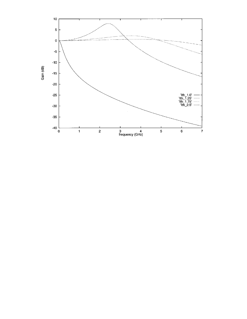
Figure 5: Small signal frequency response amplitude (Laser A or Way’s case [4]) versus frequency for various values of the bias current. From top to bottom, the bias current is taken as $I_{th}$, 1.25 $I_{th}$, 1.75 $I_{th}$ and 2.5 $I_{th}$ where $I_{th}\sim$ 21mA.

Obviously, Way’s estimation way of the resonance frequency is approximate by comparing (17) and (18) since he wanted to get an analytical estimate of the resonance frequency. In order to estimate the discrepancies between our work and Way’s we display in Figure 5 the frequency response for various values of the bias current expressed in terms of the threshold current $I_{th}\sim$21mA.

IV LARGE-SIGNAL DYNAMIC RESPONSE

We exploit three possible excitation scheme for the injection current:

1. A step excitation in order to evaluate the step response of the laser.

2. A graded response with a Gaussian time excitation towards a higher injection level.

3. A modulation injection in order to estimate the modulation response of the laser for large excursions of the injection current.

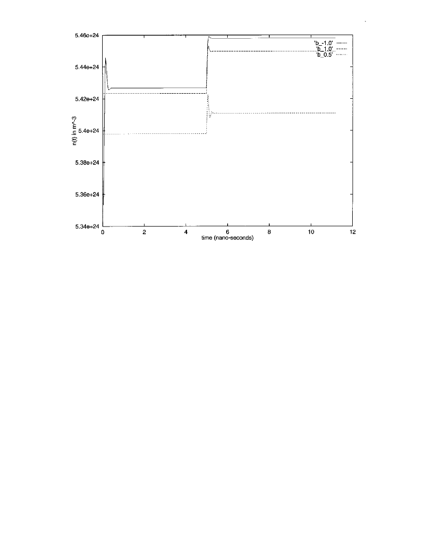
Figure 6: Laser A large signal dynamic response amplitude of the carrier density versus time for various values of b: -1.0, 0.5, 1.0. The bias current is 40 mA and a square pulse excitation of 10 mA is applied after 5 nanoseconds. The dynamic response for b=1.5 is off the graph scale.

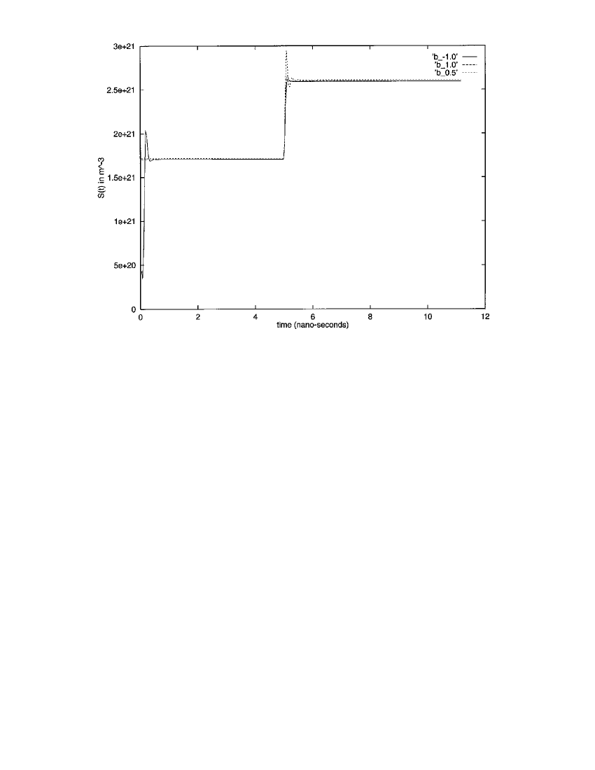
Figure 7: Laser A large signal dynamic response amplitude of the photon density versus time for various values of b: -1.0, 0.5, 1.0. The bias current is 40 mA and a square pulse excitation of 10 mA is applied after 5 nanoseconds. The dynamic response for b=1.5 is off the graph scale.

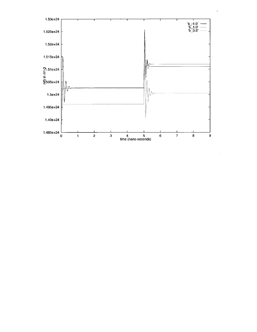
Figure 8: Laser B large signal dynamic response amplitude of the carrier density versus time for various values of b: -1.0, 0.5, 1.0. The bias current is 1 mA and a square pulse excitation of 0.5 mA is applied after 5 nanoseconds. The dynamic response for b=1.5 is off the graph scale.

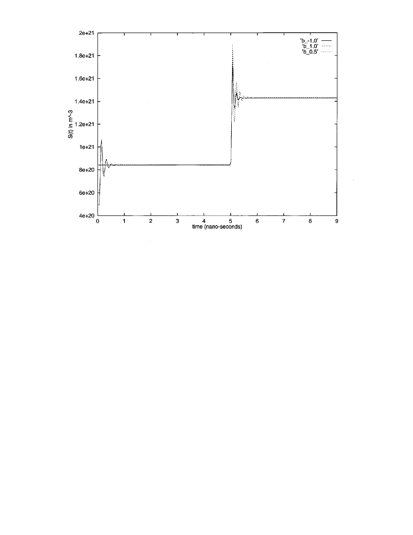
Figure 9: Laser B large signal dynamic response amplitude of the photon density versus time for various values of b: -1.0, 0.5, 1.0. The bias current is 1 mA and a square pulse excitation of 0.5 mA is applied after 5 nanoseconds. The dynamic response for b=1.5 is off the graph scale.

As an example we consider lasers A and B biased at t=0 and excited with an additional square pulse triggered after 5 nanoseconds of operation. Figures 6-9 show the large signal dynamic responses for the carrier and photon densities as functions of time for different values of b. As expected, the value of b deeply affects the dynamic response of the Laser as observed in the figures 6-9.

V CONCLUSIONS

We have developed an approach that evaluates the DC characteristics, small-signal frequency response and large- signal dynamic responses of carrier and photon densities in single-mode semiconductor laser diodes directly from the rate equations. The laser is described with a pair of rate equations containing a novel non-linear gain compensation term depending on a single parameter b that can be chosen arbitrarily in the range [0,1.5] as has been shown recently with a microscopic calculation of plasma-heating induced intensity-dependent gain effects ning .

Our DC evaluations agree with several published results agrawal ; ning ; darcie ; way ; bowers86 ; bowers87 and our large-signal dynamical reponses agree also with what is well established in the literature channin . We differ with the small-signal frequency response results given by Way way due to a discrepancy in the frequency response and resonance frequency estimation.

The parameter b has almost no effect on the DC characteristics but deeply affects the small-signal frequency response as well as the large-signal dynamic response.

The methodology developed in this work can be easily generalised to an arbitrary number of state equations that appear in multimode semiconductor lasers, MQW (Muli-Quantum- Well) or Strained layer lasers rideout ; tessler ; makino .

Acknowledgement
This work started while the author was with the Department of Electrical Engineering and with TRLabs in Saskatoon, Canada. The author wishes to acknowledge friendly discussions with David Dodds regarding some aspects of the problem. This work was supported in part by a Canada NSERC University fellowship grant.

Appendix

LASER A (ORTEL LS-620)
$G$ (mode confinement factor)	0.646
$\tau_{n}$ (electron spontaneous lifetime)	$3.72\hskip 2.84526pt10^{-9}\hskip 2.84526ptsec$
$\tau_{ph}$ (photon lifetime)	$2.10^{-12}sec$
$N_{t}$ (electron density at transparency)	$4.6\hskip 2.84526pt10^{24}m^{-3}$
$g$ (differential gain )	$10^{-12}\hskip 2.84526ptm^{3}/sec$
$\epsilon$ (gain compression parameter)	$3.8\hskip 2.84526pt10^{-23}\hskip 2.84526ptm^{3}$
$\beta$ (fraction of spontaneous emission coupled to the lasing mode)	0.001
$V$ (volume of the active region)	$9.10^{-17}m^{3}$

Table 1: Physical parameters of Laser A

LASER B
$G$ (mode confinement factor)	0.34
$\tau_{n}$ (electron spontaneous lifetime)	$3.\hskip 2.84526pt10^{-9}\hskip 2.84526ptsec$
$\tau_{ph}$ (photon lifetime)	$2.10^{-12}sec$
$N_{t}$ (electron density at transparency)	$10^{24}m^{-3}$
$g$ (differential gain )	$3.10^{-12}\hskip 2.84526ptm^{3}/sec$
$\epsilon$ (gain compression parameter)	$3.\hskip 2.84526pt10^{-23}\hskip 2.84526ptm^{3}$
$\beta$ (fraction of spontaneous emission coupled to the lasing mode)	0.001
$V$ (volume of the active region)	$3.6\hskip 2.84526pt10^{-18}m^{3}$

Table 2: Physical parameters of Laser B

Figure Captions

• $S-I$ characteristics (Laser A) for various values of b: -1.0, 0.5, 1.0 and 1.5. The different values of b do not affect significantly the DC characteristics.

• $S-I$ characteristics (Laser B) for various values of b: -1.0, 0.5, 1.0 and 1.5. The different values of b do not affect significantly the DC characteristics.

• Small signal frequency response amplitude (Laser A) versus frequency for various values of b: -1.0, 0.5, 1.0 and 1.5. The bias current is chosen to be 40 mA.

• Small signal frequency response amplitude (Laser B) versus frequency for various values of b: -1.0, 0.5, 1.0 and 1.5. The bias current is chosen to be 1 mA.

• Small signal frequency response amplitude (Laser A or Way’s case [4]) versus frequency for various values of the bias current. The bias current is taken as $I_{th}$, 1.25 $I_{th}$, 1.75 $I_{th}$ and 2.5 $I_{th}$ where $I_{th}\sim$ 21mA.

• Laser A large signal dynamic response amplitude of the carrier density versus time for various values of b: -1.0, 0.5, 1.0. The bias current is 40 mA and a square pulse excitation of 10 mA is applied after 5 nanoseconds. The dynamic response for b=1.5 is off the graph scale.

• Laser A large signal dynamic response amplitude of the photon density versus time for various values of b: -1.0, 0.5, 1.0. The bias current is 40 mA and a square pulse excitation of 10 mA is applied after 5 nanoseconds. The dynamic response for b=1.5 is off the graph scale.

• Laser B large signal dynamic response amplitude of the carrier density versus time for various values of b: -1.0, 0.5, 1.0. The bias current is 1 mA and a square pulse excitation of 0.5 mA is applied after 5 nanoseconds. The dynamic response for b=1.5 is off the graph scale.

• Laser B large signal dynamic response amplitude of the photon density versus time for various values of b: -1.0, 0.5, 1.0. The bias current is 1 mA and a square pulse excitation of 0.5 mA is applied after 5 nanoseconds. The dynamic response for b=1.5 is off the graph scale.

References

- (1) G.P Agrawal: IEEE Photon. Technology Letters PTL-1, 419 (1989).
- (2) C.Z Ning and J.V Moloney: App. Phys. Lett. 66, 559 (1995).
- (3) T.E. Darcie, R. S . Tucker and G.J. Sullivan: Electronics Letters 21, 665 (1985). See also: Erratum in Electronics Letters 22, 619 (1986).
- (4) W.I. Way: IEEE J. of Lightwave Technology LT-5, 305 (1987).
- (5) J. E. Bowers, B. Roe Hemenway, A. H. Gnauck and D. Wilt: IEEE J. Quantum Electronics QE-22, 833 (1986).
- (6) J.E. Bowers: Sol. State Electronics 30, 1 (1987).
- (7) D. J. Channin: J. App. Phys. 50, 3858 (1979).
- (8) W. Rideout, W. F. Sharfin, E.S. Koteles, M. O. Vassel and B. Elman: IEEE Photon. Technology Letters PTL-3, 784 (1991).
- (9) N. Tessler, R. Nagar and G. Eisenstein: IEEE J. Quantum Electronics QE-28, 2242 (1992).
- (10) G.P. Li, T. Makino, R. Moore, N. Puetz, K.W Leong and H. Lu: IEEE J. Quantum Electronics QE-29, 1736 (1993).
- (11) Press, W. H., Flannery, B. P., Teukolsky, S. A. and Vetterling W. T., Numerical Recipes in C , Cambridge University Press, 1989.