QED self-energy contribution to highly-excited atomic states

Abstract

We present numerical values for the self-energy shifts predicted by QED (Quantum Electrodynamics) for hydrogenlike ions (nuclear charge $60\leq Z\leq 110$) with an electron in an $n=3$, $4$ or $5$ level with high angular momentum ($5/2\leq j\leq 9/2$). Applications include predictions of precision transition energies and studies of the outer-shell structure of atoms and ions.

I Introduction

The one-loop self-energy is the largest radiative correction in atoms and ions. It has been known for many years that for high nuclear charge $Z$, results obtained by a perturbation expansion in the number of interactions with the nucleus, i.e., in powers of $Z\alpha$ are not accurate. There are many recent examples in which self-energy shifts for high principal quantum numbers and/or angular momenta are needed. For example, the outer-shell structure of very heavy elements is being studied to determine electron affinities or chemical properties. Similarly, transitions within the ground configuration of the Ti-like iso-electronic sequence (with outer-shell structure $3d^{4}$) have been measured for very high nuclear charges $Z$ [1, 2, 3, 4, 5, 6, 7], with results that differ systematically from theoretical calculations [8, 9, 10, 11] that do not include the self-energy correction for the $3d_{5/2}$ level beyond the Bethe logarithm and lowest-order electron anomalous moment. The same is true for systematic studies of magnesiumlike ions [12]. Yet it has been shown recently that effects beyond the lowest order are large at high $Z$, even for rather large $n$ and angular momenta [13]. Several calculations have thus been undertaken. Preliminary results have been reported for the $6s$ and $8d_{3/2}$ shells [13], while Labzowski et al. [14] and Yerokhin and Shabaev [15] have calculated a limited number of self-energy level shifts with methods developed recently. In this paper, we provide accurate calculations for nuclear charge $Z$ in the range $60\leq Z\leq 110$ for an electron in a level with $n=3$, $4$, or $5$ with high angular momentum ($5/2\leq j\leq 9/2$). The results increase considerably the number of atoms for which the exact one-loop self-energy is available.

After the seminal works of Brown et al. [16] and of Desiderio and Johnson [17], one of us (PJM) developed an efficient method for evaluating the self-energy level shifts in a framework where the electron-nucleus interaction is treated non-perturbatively. This method was first applied to the $1s$ level of one-electron atoms [18, 19]. Later, the self-energy contribution to the Lamb shift of the $2s$ and $2p_{1/2}$ states was studied [20], and subsequently, all levels with principal quantum number $n=2$ were evaluated with higher accuracy [21]. Additional excited states with $3\leq n\leq 5$ and angular momentum $j\leq 3/2$ were studied more recently in Ref. [22], where the difficulties which arise for highly-excited states are described and solved for low angular momenta. Self-energy calculations for states with angular momentum $j>3/2$ has been a long standing problem since the publication of the original method [18].

In the present paper we extend the self-energy calculation methods developed in [18, 19, 20, 21, 22] to arbitrary angular momenta. We derive general, numerically efficient formulas for the angular integrals that appear in self-energy expressions; these integrals were only known for states with $j\leq 3/2$. We perform calculations for $5/2\leq j\leq 9/2$ and for principal quantum numbers $n=3$, $4$ and $5$. The numerically efficient renormalization technique described in Refs. [23, 24] is used, as its formulation is independent of the atomic level. This method yields precise results for the self-energy shifts; other groups have published numerical results based on various numerical strategies that give less precise values [25, 26, 27].

The implementation of our formulas on a computer is simple, since the only mathematical objects used in our final expressions are Bessel functions of the first kind and (squared) Wigner $3j$ symbols with all angular momentum projections set to zero. Our expressions are optimized for numerical calculations and have proved to yield very accurate results. Our formulas for electrons with angular momentum $j=3/2$ differ from known expressions [21, 28], because we have adapted our results to more accurate numerical calculations.

The outline of the paper is as follows. In Sec. II, we recall the principle of the self-energy calculation we use. In Sec. III we summarize our formulas for the self-energy angular integrals, which constitute the main analytical result of the present work. In Sec. IV we present numerical results for levels $d_{5/2}$, $f_{5/2}$, $f_{7/2}$, $g_{7/2}$ and $g_{9/2}$ with principal quantum numbers $3\leq n\leq 5$. Detailed derivations of the formulas presented in Sec. III are given in Sec. V, while derivations by a different method, used for checking purposes, are presented in Sec. VI. Section VII concludes the paper.

Throughout this article, we use the convention $\sum_{i=a}^{b}\equiv 0$ whenever $a>b$.

II Self-energy shift formula

The expression for the self-energy shift of an electronic state $n$ can be written for a large class of potentials ${\cal V}(\mathchoice{{\hbox{\boldmath$\displaystyle x$}}}{{\hbox{\boldmath$\textstyle x$}}}{{\hbox{\boldmath$\scriptstyle x$}}}{{\hbox{\boldmath$\scriptscriptstyle x$}}})$ as the sum

$${\cal E}_{\rm SE}\equiv{\cal E}_{\rm L}+{\cal E}_{\rm H}$$ (1)

of a low-energy part ${\cal E}_{\rm L}$ and a high-energy part ${\cal E}_{\rm H}$ given (in units in which $\hbar=c=m_{\rm e}=1)$ by [18]

$${\cal E}_{\rm L}\equiv\frac{\alpha}{\pi}{\cal E}_{n}-\frac{\alpha}{\pi}{\mathrm{P}}\!\int_{0}^{{\cal E}_{n}}dz\int d\mathchoice{{\hbox{\boldmath$\displaystyle x$}}}{{\hbox{\boldmath$\textstyle x$}}}{{\hbox{\boldmath$\scriptstyle x$}}}{{\hbox{\boldmath$\scriptscriptstyle x$}}}_{2}\int d\mathchoice{{\hbox{\boldmath$\displaystyle x$}}}{{\hbox{\boldmath$\textstyle x$}}}{{\hbox{\boldmath$\scriptstyle x$}}}{{\hbox{\boldmath$\scriptscriptstyle x$}}}_{1}\,\varphi_{n}^{\dagger}(\mathchoice{{\hbox{\boldmath$\displaystyle x$}}}{{\hbox{\boldmath$\textstyle x$}}}{{\hbox{\boldmath$\scriptstyle x$}}}{{\hbox{\boldmath$\scriptscriptstyle x$}}}_{2})\alpha^{l}{\cal G}(\mathchoice{{\hbox{\boldmath$\displaystyle x$}}}{{\hbox{\boldmath$\textstyle x$}}}{{\hbox{\boldmath$\scriptstyle x$}}}{{\hbox{\boldmath$\scriptscriptstyle x$}}}_{2},\mathchoice{{\hbox{\boldmath$\displaystyle x$}}}{{\hbox{\boldmath$\textstyle x$}}}{{\hbox{\boldmath$\scriptstyle x$}}}{{\hbox{\boldmath$\scriptscriptstyle x$}}}_{1},z)\alpha^{m}\varphi_{n}(\mathchoice{{\hbox{\boldmath$\displaystyle x$}}}{{\hbox{\boldmath$\textstyle x$}}}{{\hbox{\boldmath$\scriptstyle x$}}}{{\hbox{\boldmath$\scriptscriptstyle x$}}}_{1})(\delta_{l,m}\mathchoice{{\hbox{\boldmath$\displaystyle\nabla$}}}{{\hbox{\boldmath$\textstyle\nabla$}}}{{\hbox{\boldmath$\scriptstyle\nabla$}}}{{\hbox{\boldmath$\scriptscriptstyle\nabla$}}}_{2}\cdot\mathchoice{{\hbox{\boldmath$\displaystyle\nabla$}}}{{\hbox{\boldmath$\textstyle\nabla$}}}{{\hbox{\boldmath$\scriptstyle\nabla$}}}{{\hbox{\boldmath$\scriptscriptstyle\nabla$}}}_{1}-\nabla_{2}^{l}\nabla_{1}^{m})\frac{\sin[({\cal E}_{n}-z)x_{21}]}{({\cal E}_{n}-z)^{2}x_{21}}$$ (2)

and

$$\ {\cal E}_{\rm H}\equiv\frac{\alpha}{2\pi{i}}\int_{\rm C_{H}}dz\ \int d\mathchoice{{\hbox{\boldmath$\displaystyle x$}}}{{\hbox{\boldmath$\textstyle x$}}}{{\hbox{\boldmath$\scriptstyle x$}}}{{\hbox{\boldmath$\scriptscriptstyle x$}}}_{2}\int d\mathchoice{{\hbox{\boldmath$\displaystyle x$}}}{{\hbox{\boldmath$\textstyle x$}}}{{\hbox{\boldmath$\scriptstyle x$}}}{{\hbox{\boldmath$\scriptscriptstyle x$}}}_{1}\,\varphi_{n}^{\dagger}(\mathchoice{{\hbox{\boldmath$\displaystyle x$}}}{{\hbox{\boldmath$\textstyle x$}}}{{\hbox{\boldmath$\scriptstyle x$}}}{{\hbox{\boldmath$\scriptscriptstyle x$}}}_{2})\alpha_{\mu}{\cal G}(\mathchoice{{\hbox{\boldmath$\displaystyle x$}}}{{\hbox{\boldmath$\textstyle x$}}}{{\hbox{\boldmath$\scriptstyle x$}}}{{\hbox{\boldmath$\scriptscriptstyle x$}}}_{2},\mathchoice{{\hbox{\boldmath$\displaystyle x$}}}{{\hbox{\boldmath$\textstyle x$}}}{{\hbox{\boldmath$\scriptstyle x$}}}{{\hbox{\boldmath$\scriptscriptstyle x$}}}_{1},z)\alpha^{\mu}\varphi_{n}(\mathchoice{{\hbox{\boldmath$\displaystyle x$}}}{{\hbox{\boldmath$\textstyle x$}}}{{\hbox{\boldmath$\scriptstyle x$}}}{{\hbox{\boldmath$\scriptscriptstyle x$}}}_{1})\frac{e^{-bx_{21}}}{x_{21}}-\delta m\int d\mathchoice{{\hbox{\boldmath$\displaystyle x$}}}{{\hbox{\boldmath$\textstyle x$}}}{{\hbox{\boldmath$\scriptstyle x$}}}{{\hbox{\boldmath$\scriptscriptstyle x$}}}\ \varphi_{n}^{\dagger}(\mathchoice{{\hbox{\boldmath$\displaystyle x$}}}{{\hbox{\boldmath$\textstyle x$}}}{{\hbox{\boldmath$\scriptstyle x$}}}{{\hbox{\boldmath$\scriptscriptstyle x$}}})\beta\varphi_{n}(\mathchoice{{\hbox{\boldmath$\displaystyle x$}}}{{\hbox{\boldmath$\textstyle x$}}}{{\hbox{\boldmath$\scriptstyle x$}}}{{\hbox{\boldmath$\scriptscriptstyle x$}}}),$$ (3)

where $b\equiv-i\left[({\cal E}_{n}-z)^{2}+i\epsilon\right]^{1/2}$, ${\rm Re}(b)>0$ is the photon energy, and $x_{21}\equiv||\mathchoice{{\hbox{\boldmath$\displaystyle x$}}}{{\hbox{\boldmath$\textstyle x$}}}{{\hbox{\boldmath$\scriptstyle x$}}}{{\hbox{\boldmath$\scriptscriptstyle x$}}}_{2}-\mathchoice{{\hbox{\boldmath$\displaystyle x$}}}{{\hbox{\boldmath$\textstyle x$}}}{{\hbox{\boldmath$\scriptstyle x$}}}{{\hbox{\boldmath$\scriptscriptstyle x$}}}_{1}||$ ($\epsilon$ is an infinitesimal positive quantity). In these expressions, $\varphi_{n}$ and ${\cal E}_{n}$ are the eigenfunction and eigenvalue of the Dirac equation for the bound state $n$, and ${\cal G}$ is the Dirac Green’s function: ${\cal G}(z)=({\cal H}-z)^{-1}$, where ${\cal H}=\mathchoice{{\hbox{\boldmath$\displaystyle\alpha$}}}{{\hbox{\boldmath$\textstyle\alpha$}}}{{\hbox{\boldmath$\scriptstyle\alpha$}}}{{\hbox{\boldmath$\scriptscriptstyle\alpha$}}}\cdot\mathchoice{{\hbox{\boldmath$\displaystyle p$}}}{{\hbox{\boldmath$\textstyle p$}}}{{\hbox{\boldmath$\scriptstyle p$}}}{{\hbox{\boldmath$\scriptscriptstyle p$}}}+{\cal V}+\beta$ is the Dirac Hamiltonian. Indices $l$ and $m$ are summed from 1 to 3, and index $\mu$ is summed from 0 to 3. The contour ${\rm C_{H}}$ extends from $-i\infty$ to $0-i\epsilon$ and from $0+i\epsilon$ to $+i\infty$.

Since the high-energy part and the renormalization procedure described in Refs. [21, 22, 23, 24] are already known for arbitrary angular momenta, this paper is concerned with the low-energy part (2). For a spherically symmetric potential ${\mathcal{V}}$, a separation of the photon propagator and of Dirac wavefunctions into radial and angular parts yields the following expression for the low-energy part of the self-energy:

$${\mathcal{E}}_{L}=\frac{\alpha}{\pi}{\mathcal{E}}_{n}-\frac{\alpha}{\pi}{\mathrm{P}}\int_{0}^{{\mathcal{E}}_{n}}dz\int_{0}^{\infty}dx_{2}x_{2}^{2}\int_{0}^{\infty}dx_{1}x_{1}^{2}$$ (4)

$$\times\sum_{\kappa}\sum_{i,j=1}^{2}f_{\overline{\imath}}(x_{2})G_{\kappa}^{ij}(x_{2},x_{1},z)f_{\overline{\jmath}}(x_{1})A_{\kappa,\kappa_{n}}^{ij}(x_{2},x_{1}),$$ (5)

where the $f_{i}$’s are the radial components of the wavefunction $\varphi_{n}$, $\bar{\imath}\equiv 3-i$, $G_{\kappa}^{ij}$ are the radial components of the Green’s functions, and $A_{\kappa,\kappa_{n}}^{ij}$ are functions that contain angular integrations as well as the photon propagator. The Dirac angular quantum number of the electron for which the self-energy is calculated is denoted by $\kappa_{n}$. Detailed definitions of these notations can be found in Ref. [18].

Expression (5) can for instance be applied to a pure Coulomb potential ${\mathcal{V}}$ or to the self-energy screening correction [29]. The potential ${\mathcal{V}}$ affects the radial components $f$ and $G$; on the contrary, the angular coefficients $A$ are independent of ${\mathcal{V}}$; this paper provides analytical formulas for these coefficients.

III Final formulas for the angular integrals

In this section, we present our final formulas for the angular coefficients $A^{ij}_{\kappa,\kappa_{n}}$ introduced in Eq. (5). Our results can be directly implemented on a computer. Derivations of the results presented here can be found in Sec. V A and Sec. V B.

We present successively our results for the coefficients $A^{11}_{\kappa,\kappa_{n}}$ and $A^{12}_{\kappa,\kappa_{n}}$. The other two coefficients can be obtained through the following symmetries [18]:

$$A^{21}_{\kappa,\kappa_{n}} = A^{12}_{-\kappa,-\kappa_{n}}$$

$$A^{22}_{\kappa,\kappa_{n}} = A^{11}_{-\kappa,-\kappa_{n}}.$$

A Final result for $A^{11}_{\kappa,\kappa_{n}}$

1 Initial expression and notations

We give in this section the numerically optimized form that we found for the angular coefficient $A^{11}_{\kappa,\kappa_{n}}$. The most general formula available for this coefficient is [18]

$$A^{11}_{\kappa,\kappa_{n}} \equiv |\kappa|\int_{-1}^{1}\!d\xi\,\bigg{[}P_{l_{\kappa}}(\xi)P_{l_{\kappa_{n}-1}}(\xi)b^{2}T(\rho)$$ (7)

$${}-\frac{1}{\kappa\kappa_{n}}(1-\xi^{2})P^{\prime}_{l_{\kappa}}(\xi)P^{\prime}_{l_{\kappa_{n}-1}}(\xi)\frac{1}{\rho}\frac{d}{d\rho}T(\rho)\bigg{]},$$

where $P_{n}$ is the Legendre polynomial [30] of degree $n$, and where

$$l_{\kappa}\equiv|\kappa+1/2|-1/2$$ (8)

denotes the orbital angular momentum associated with the Dirac angular quantum number $\kappa$; the other functions are defined as:

$$\rho(x_{1},x_{2},\xi)\equiv\sqrt{x_{1}^{2}+x_{2}^{2}-2x_{1}x_{2}\xi}$$ (9)

and

$$T(\rho)\equiv\sin(b\rho)/(b^{2}\rho).$$ (10)

The quantities $\kappa_{n}$, $\kappa$, $x_{1}$, $x_{2}$ and $b$ are considered here as fixed parameters. Since distances $x_{1}$ and $x_{2}$ often appear multiplied by the energy $b$, we define

$\displaystyle y_{1}\equiv b\,x_{1}\mbox{ and }y_{2}\equiv b\,x_{2}.$

It is also convenient to introduce the notation

$\displaystyle{\mathcal{J}}^{2}_{l}\equiv l(l+1)$

for the eigenvalues of the squared angular momentum operator in terms of the angular momentum $l$.

2 Result of the analytical integration

With the above notations, our result for the integration in Eq. (8) reads:

$$A^{11}_{\kappa,\kappa_{n}} = \sum_{\makebox[0.0pt]{$\scriptstyle l=|l_{\kappa}-l_{-\kappa_{n}}|$}}^{\makebox[0.0pt]{$\scriptstyle l_{\kappa}+l_{-\kappa_{n}}$}}(2l+1)|\kappa|\Bigg{[}2b\left(\begin{array}[]{ccc}l_{\kappa}&l_{-\kappa_{n}}&l\\ 0&0&0\end{array}\right)^{2}j_{l}(y_{1})j_{l}(y_{2})$$ (14)

$$\qquad+\frac{1}{\kappa\kappa_{n}}{\mathcal{L}}(l,l_{\kappa},l_{-\kappa_{n}})\frac{j_{l}(y_{1})}{y_{1}}\frac{j_{l}(y_{2})}{x_{2}}\Bigg{]},$$

where the $2\times 3$ matrices are Wigner $3j$-coefficients, where the $j_{l}$’s are the spherical Bessel functions of the first kind [30], and where we have introduced a symbol for the following quantity:

$${\mathcal{L}}(a,b,c)\equiv\left\{\begin{array}[]{l}\displaystyle\sum_{\parbox{60.27771pt}{ \centering\par$i=|a-b|$\\ $i+|a-b|$ even \par\@add@centering}}^{c-1}\left(\begin{array}[]{ccc}a&b&i\\ 0&0&0\end{array}\right)^{2}(2i+1)({\mathcal{J}}^{2}_{a}+{\mathcal{J}}^{2}_{b}-{\mathcal{J}}^{2}_{i})\quad\mbox{if $a+b+c$ odd}\\ \\ 0\quad\mbox{otherwise.}\end{array}\right.$$ (15)

Despite the non-symmetrical form (15), the quantity ${\mathcal{L}}(a,b,c)$ is totally symmetrical with respect to any permutation of its arguments, as we prove in Sec. V A 2.

3 Numerical implementation

Equation (14) can be readily implemented on a computer. In Eq. (14), no term is singular (with respect to the parameters $b$, $x_{1}$ and $x_{2}$). In fact, the expansion of the Bessel functions about the origin [30] is such that $j_{l}(z)={\mathcal{O}}(z^{l})$; singularities could appear only through $j_{0}(z)/z$, which is singular as $z\rightarrow 0$. But $l=0$ imposes that $l+l_{\kappa}+l_{-\kappa_{n}}$ be even, so that $j_{0}(z)/z$ is actually never used in Eq. (14).

Since the number of terms in Eq. (15) is smaller than $c$, we have decided to set $c=l_{-\kappa_{n}}$ in Eq. (14), because $l_{-\kappa_{n}}$ is small, being the orbital momentum of the level for which the self-energy is calculated [18]. Furthermore, we note that in Eq. (14), for a given $l$, only one term inside the brackets contribute to $A^{11}_{\kappa,\kappa_{n}}$ because of parity selection on Wigner $3j$-coefficients [31] and in our quantity ${\mathcal{L}}(a,b,c)$ of Eq. (15).

We have also checked whether result (14) could yield strong numerical cancellations in the following ranges of parameters

$$\begin{array}[]{c}b\in[0,1],\,x_{1},x_{2}\in[0,100],\\ |\kappa_{n}|\in[1,10]\mbox{\ and\ }|\kappa|\in[1,1000],\end{array}$$ (16)

which are typical of the values used in numerical calculations [18]. We checked for possible cancellations with an arbitrary precision in the following two cases: (a) two numbers add up to a very small one (about $10^{-8}$ smaller than the two numbers); (b) a large number is added to a number which is much smaller (by a factor of $10^{-9}$). Our checks have shown that no such numerical problems arise with the terms of Eq. (14) when the summation is done by starting from the higher limit $l_{\kappa}+l_{-\kappa_{n}}$; this choice of summation order is numerically motivated by the over-exponential damping of the spherical Bessel functions of the first kind [32]:

$$j_{l}(z)\sim\frac{1}{2^{3/2}l}{\left(\frac{ez}{2l}\right)}^{l}$$ (17)

when $l>ez/2$; thus, summing the terms of the final result (14) with decreasing $l$’s allows one to include larger and larger terms in the total sum, which is necessary for obtaining accurate numerical sums.

We have numerically tested formula (14) against Mathematica, against the alternate formula presented below [Eq. (94)] and against Mohr’s implementation of his special cases $|\kappa_{n}|\leq 2$; we have found excellent accuracy in the parameter ranges used in the low-energy part calculations of the self-energy [18, 21, 22], i.e., in the range of parameters reached by our calculations of the self-energy in ions with $Z\geq 10$:

$$\begin{array}[]{c}b\in[0,1],\,x_{1},x_{2}\in[0,5000],\\ |\kappa_{n}|\in[1,5]\mbox{\ and\ }|\kappa|\in[1,5000].\end{array}$$ (18)

B Final result for $A^{12}_{\kappa,\kappa_{n}}$

1 General integration result

We give in this section a form of the angular coefficient $A^{12}_{\kappa,\kappa_{n}}$ which is optimized for numerical calculations. We start from the most general formula available [18] for this angular coefficient:

$$A^{12}_{\kappa,\kappa_{n}} \equiv -|\kappa|\int_{-1}^{1}\!d\xi\,\bigg{\{}\left[P_{l_{\kappa-1}}(\xi)P_{l_{\kappa_{n}}}(\xi)-\frac{1}{\kappa\kappa_{n}}(1-\xi^{2})P^{\prime}_{l_{\kappa-1}}(\xi)P^{\prime}_{l_{\kappa_{n}}}(\xi)\right]\frac{1}{\rho}\frac{d}{d\rho}T(\rho)$$ (20)

$$\qquad\qquad\quad+[x_{2}P_{l_{\kappa-1}}(\xi)-x_{1}P_{l_{\kappa}}(\xi)][x_{2}P_{l_{\kappa_{n}}}(\xi)-x_{1}P_{l_{\kappa_{n}-1}}(\xi)]\frac{1}{\rho}\frac{d}{d\rho}\frac{1}{\rho}\frac{d}{d\rho}T(\rho)\bigg{\}}.$$

With the help of the notations defined previously, the (almost) final result of our calculation of Eq. (20) reads

$$A^{12}_{\kappa,\kappa_{n}} = \sum_{\parbox{60.27771pt}{ \centering\par$l=|l_{\kappa}-l_{\kappa_{n}}|$\\ $l+l_{\kappa}+l_{\kappa_{n}}$ even \@add@centering}}^{l_{\kappa}+l_{\kappa_{n}}}\frac{j_{l}(y_{1})}{y_{1}}\frac{j_{l}(y_{2})}{x_{2}}\frac{|\kappa|}{\kappa\kappa_{n}}(2l+1)\Bigg{\{}\left(\begin{array}[]{ccc}l_{\kappa_{n}}&l_{\kappa}&l\\ 0&0&0\end{array}\right)^{2}[{\mathcal{J}}^{2}_{\kappa_{n}}({\mathcal{J}}^{2}_{l}+{\mathcal{J}}^{2}_{\kappa}-{\mathcal{J}}^{2}_{\kappa_{n}})+\kappa^{2}({\mathcal{J}}^{2}_{l}-{\mathcal{J}}^{2}_{\kappa}+{\mathcal{J}}^{2}_{\kappa_{n}})]$$ (28)

$$\qquad\quad{}-{\mathcal{L}}(l,l_{-\kappa},l_{\kappa_{n}})\Bigg{\}}$$

$$\qquad{}+|\kappa|(2l+1)\left(\begin{array}[]{ccc}l_{\kappa_{n}}&l_{\kappa}&l\\ 0&0&0\end{array}\right)^{2}\times\Bigg{[}j_{l}^{\prime}(y_{1})\frac{j_{l}(y_{2})}{x_{2}}({\mathcal{J}}^{2}_{l}-{\mathcal{J}}^{2}_{\kappa}+{\mathcal{J}}^{2}_{\kappa_{n}})/\kappa_{n}$$

$$\qquad\quad{}+\frac{j_{l}(y_{1})}{x_{1}}j_{l}^{\prime}(y_{2})({\mathcal{J}}^{2}_{l}+{\mathcal{J}}^{2}_{\kappa}-{\mathcal{J}}^{2}_{\kappa_{n}})/\kappa+j_{l}^{\prime}(y_{1})j_{l}^{\prime}(y_{2})\times 2b\Bigg{]},$$

which is the generalization to any atomic state of the angular coefficient $A^{12}_{\kappa,\kappa_{n}}$ of the low-energy part of the self-energy [18]. Equation (28) has a few crucial computational advantages: (a) all the sums contain a finite number of terms; (b) there are no large terms due to small $b$, $x_{1}$ or $x_{2}$; in fact, it is easy to see that the only divergent quantities can come from $j_{l=0}(z)/z$, but that this quantity is actually always multiplied by 0. We thus gain numerical accuracy compared to the published formulas [21, 22] for the special cases $\kappa_{n}=\pm 2$.

2 Numerical optimization

As for $A^{11}_{\kappa,\kappa_{n}}$, we have checked whether result (28) yields strong numerical cancellations in the parameter ranges defined by (16). Our checks have shown that no such numerical problems arise with the terms of Eq. (28) [evaluated in the order indicated by the parentheses, with summations done from the higher limit because of Eq. (17)], except sometimes for the minimum $l$, i.e., for

$\displaystyle l=l_{\mathrm{m}in}\equiv|l_{\kappa}-l_{\kappa_{n}}|.$

However, we have cured this disease by noticing patterns in the way numerical cancellation appear: we have experimentally found four different areas of the $(\kappa,\kappa_{n})$ plane, defined by which of the terms of Eq. (28) cancel each other; the “terms” are defined here by separating terms with zero, one and two derivatives of Bessel functions: we select the four terms of Eq. (28) associated with $[j_{l_{\mathrm{m}in}}(y_{1})/y_{1}][j_{l_{\mathrm{m}in}}(y_{2})/x_{2}]$, $j_{l_{\mathrm{m}in}}^{\prime}(y_{1})[j_{l_{\mathrm{m}in}}(y_{2})/x_{2}]$, $[j_{l_{\mathrm{m}in}}(y_{1})/x_{1}]j_{l_{\mathrm{m}in}}^{\prime}(y_{2})$, and $j_{l_{\mathrm{m}in}}^{\prime}(y_{1})j_{l_{\mathrm{m}in}}^{\prime}(y_{2})$.

By using explicit polynomial formulas for the orbital angular momenta $l_{\kappa}$ and $l_{\kappa_{n}}$ in each region, it is possible to obtain simplified expressions for the four terms of Eq. (28); terms can then generally be grouped together [in a way that depends on the area in which $(\kappa,\kappa_{n})$ lies] through the Bessel identity [30]

$$\frac{l}{z}j_{l}(z)-j_{l}^{\prime}(z)=j_{l+1}(z).$$ (29)

We have found numerically that this identity can yield very strong numerical cancellations between the $l=l_{\mathrm{m}in}$ terms of Eq. (28).

Thus, we have mathematically found the equations of the four cancellation areas, and we have used identity (29) in order to express the final result in terms of the right-hand side of Eq. (29) instead of numerically calculating the left-hand side of the identity. The precise shapes of the areas in the $(\kappa,\kappa_{n})$ plane are

$$\begin{array}[]{ll}\mbox{area 1:}&\kappa\kappa_{n}<0\mbox{ and }\kappa(l_{\kappa}-l_{\kappa_{n}})\leq 0\\ \mbox{area 2:}&\kappa\kappa_{n}<0\mbox{ and }\kappa(l_{\kappa}-l_{\kappa_{n}})>0\\ \mbox{area 3:}&\kappa\kappa_{n}>0\mbox{ and }\kappa(l_{\kappa}-l_{\kappa_{n}})\leq 0\\ \mbox{area 4:}&\kappa\kappa_{n}>0\mbox{ and }\kappa(l_{\kappa}-l_{\kappa_{n}})>0.\end{array}$$ (30)

A numerical implementation of Eq. (28) should thus calculate the terms corresponding to $l=l_{\mathrm{m}in}$ with the following expressions, which depend on the area in which $(\kappa,\kappa_{n})$ lies:

$$A^{12}_{\kappa,\kappa_{n}}(l=l_{\mathrm{m}in})=\left\{\begin{array}[]{ll}2b|\kappa|(2l_{\mathrm{m}in}+1)\left(\begin{array}[]{ccc}l_{\kappa_{n}}&l_{\kappa}&l_{\mathrm{m}in}\\ 0&0&0\end{array}\right)^{2}j_{l_{\mathrm{m}in}+1}(y_{1})j_{l_{\mathrm{m}in}+1}(y_{2})&\mbox{in area 1}\\ A^{12}_{\kappa,\kappa_{n}}(l=l_{\mathrm{m}in})\mbox{ from Eq.~{}(\ref{eq:a12final})}&\mbox{in area 2}\\ \left(\begin{array}[]{l}-|\kappa|(2l_{\mathrm{m}in}+1)\left(\begin{array}[]{ccc}l_{\kappa_{n}}&l_{\kappa}&l_{\mathrm{m}in}\\ 0&0&0\end{array}\right)^{2}j_{l_{\mathrm{m}in}+1}(y_{1})\\ \qquad\qquad\times\left\{[j_{l_{\mathrm{m}in}}(y_{2})/x_{2}]({\mathcal{J}}^{2}_{l_{\mathrm{m}in}}-{\mathcal{J}}^{2}_{\kappa}+{\mathcal{J}}^{2}_{\kappa_{n}})/\kappa_{n}+2bj_{l_{\mathrm{m}in}}^{\prime}(y_{2})\right\}\end{array}\right)&\mbox{in area 3}\\ \left(\begin{array}[]{l}-|\kappa|(2l_{\mathrm{m}in}+1)\left(\begin{array}[]{ccc}l_{\kappa_{n}}&l_{\kappa}&l_{\mathrm{m}in}\\ 0&0&0\end{array}\right)^{2}j_{l_{\mathrm{m}in}+1}(y_{2})\\ \qquad\qquad\times\left\{[j_{l_{\mathrm{m}in}}(y_{1})/x_{1}]({\mathcal{J}}^{2}_{l_{\mathrm{m}in}}+{\mathcal{J}}^{2}_{\kappa}-{\mathcal{J}}^{2}_{\kappa_{n}})/\kappa+2bj_{l_{\mathrm{m}in}}^{\prime}(y_{1})\right\}\end{array}\right)&\mbox{in area 4}.\end{array}\right.$$ (31)

Furthermore, no factor of the form $j_{0}(z)/z$, which diverges as $z\rightarrow 0$ appears anymore in our formulas for $A^{12}_{\kappa,\kappa_{n}}$: such a factor can only be found in the $l=l_{\mathrm{m}in}$ term of result (28); but Eq. (31) must be used for this term. $l_{\mathrm{m}in}\equiv|l_{\kappa}-l_{\kappa_{n}}|$ is obviously never encountered in the first two areas of Eq. (31). In the last two areas of Eq. (31), $j_{0}(z)/z$ is used but multiplied by a factor zero, as can be seen by using the fact that $\kappa\kappa_{n}>0$.

In summary, Eqs. (28) and (31) give numerically optimized formulas for the angle coefficient $A^{12}_{\kappa,\kappa_{n}}$ of Eq. (20). We have numerically tested these formulas against Mathematica, against the alternate formula presented below [Eq. (114)], and against Mohr’s implementation of his special cases $|\kappa_{n}|\leq 2$; we have found excellent accuracy in the physical parameter ranges (18).

IV Numerical results for the self-energy

The formulas (14), (28) and (31) presented above allow us to numerically evaluate the QED self-energy contribution ${\mathcal{E}}_{\mathrm{L}}$ formally expressed in Eq. (5). The other self-energy contribution [${\mathcal{E}}_{\mathrm{H}}$, Eq. (3)] can be calculated for an arbitrary electronic state by means of previously published methods [21]. We present in this section numerical evaluations of the self-energy of atomic electrons with principal quantum number $3\leq n\leq 5$ and with angular number $3\leq|\kappa|\leq 5$, in hydrogenlike ions with nuclear charge $60\leq Z\leq 110$. We used a Fortran implementation of formulas (14), (28) and (31), as well as previously published numerical procedures [19, 21, 22, 23, 24, 29, 33, 34].

Numerical results are most conveniently expressed in terms of the usual scaled self-energy $F$:

$${\mathcal{E}}_{\mathrm{S}E}\equiv\frac{\alpha}{\pi}\frac{(Z\alpha)^{4}}{n^{3}}F(Z\alpha){m_{\mathrm{e}}c^{2}},$$ (32)

where ${\mathcal{E}}_{\mathrm{S}E}$ is the self-energy shift (1). Our evaluations of the scaled value $F$ are presented in Tables I–IV. When represented as a function of $Z\alpha$, our values display smooth curves, as can be seen in Figs. 1–5.

From Figs. 1–3, we notice that the scaled self-energy does not greatly depend on the atomic level $n$; put in other words, the $n$-dependence of the self-energy is quite well captured by the scaling $1/n^{3}$ of Eq. (32), as has been observed for $s$ and $d_{3/2}$ levels [13]. On the practical side, the slow variation of the scaled self-energy $F$ with respect to $n$ allows one to use the values we present here as estimates for higher levels $n$.

We have also grouped self-energy values by atomic level $n$ in Figs. 4 and 5. We notice that states with identical orbital angular momenta have self-energy curves that look parallel on the scale we used. This property can be understood for low nuclear charge $Z$, since states other than $s$ states have the property that $F$ is dominated in this region by a function of the form

$\displaystyle A_{40}+(Z\alpha)^{2}\log[(Z\alpha)^{-2}]A_{61}$

for $Z\alpha\ll 1$, and where $A_{40}$ and $A_{61}$ are the usual coefficients of the semi-analytic expansion of the self-energy shift [35]. (The $(Z\alpha)^{2}A_{60}$ contribution is negligible for $Z\alpha\rightarrow 0$: $(Z\alpha)^{2}=o[(Z\alpha)^{2}\log([Z\alpha]^{-2})]$.) It turns out that for $d,f,g$…  states, $A_{61}$ depends only on the orbital angular momentum (This is due to the smooth behavior of the wavefunction of such states at the origin [36].); as a consequence, the self-energy curves for states with identical quantum numbers $n$ and $l$ (angular momentum) are parallel in the limit $Z\alpha\rightarrow 0$. For the higher $Z$ values of the results we present here, the expansion of $F$ in $Z\alpha$ is not supposed to hold; however our numerical values show that the difference between the scaled self-energies of two levels with the same $n$ and $l$ varies only on the level of a few percents in the range $60\leq Z\leq 110$. Precisely, the difference between the self-energy $F$ for two states with identical $n$ and $l$ is well approximated by the value of this difference at the limit $Z\alpha\rightarrow 0$, which is known to be [37]

$$\lim_{Z\alpha\rightarrow 0}[F_{n,\kappa=-(l+1)}(Z\alpha)-F_{n,\kappa=l}(Z\alpha)]=\frac{1}{l(l+1)},$$ (33)

which approximates (to the level of a few percents) the splitting between states with identical $n$ and $l$ present in our results; it would be interesting to find an explanation of this property of the scaled self-energy $F$ at high $Z$. At low $Z$, the splitting (33) is due to the anomalous magnetic moment of the electron [37], and maybe does this effect dominate the splitting we observe between states of identical $n$ and $l$ in our high-$Z$ results.

Our results are coherent with the numerical results published by Yerokhin and Shabaev [25] for nuclear charges $Z=74$, $83$ and $92$, as shown in Tables V and VI. However, we note that our evaluations of the self-energy often lie below the values of [25], and that our results have uncertainties smaller by about two orders of magnitude. Furthermore, the value that lies the furthest from their error bars is that of the $5d_{5/2}$ level for $Z=74$, which is located relatively close ($-1.2$ standard deviations) from the previously published result [25].

V Calculation of the angular coefficients: method for optimized numerical evaluation

Our analytical evaluations of $A^{11}_{\kappa,\kappa_{n}}$ and $A^{12}_{\kappa,\kappa_{n}}$ [18] rest on a few cornerstones.

First, the dependence on $\xi$ of the integrands of Eqs. (8) and (20) is made simple by expanding the $T$ function with partial waves. In fact, in Eq. (9), $\rho$ is the distance between the two interaction points of the self-energy, $\xi$ being the cosine of the angle between these two points [18]; the $T$ function of Eq. (10) can therefore be expanded in partial waves [30]:

$$T[\rho(x_{1},x_{2},\xi)]=\frac{1}{b}\sum_{l\geq 0}(2l+1)P_{l}(\xi)j_{l}(y_{1})j_{l}(y_{2}),$$ (34)

where we still have

$\displaystyle y_{1}\equiv bx_{1}\mbox{ and }y_{2}\equiv bx_{2}.$

Thus, integrals of terms of Eqs. (8) and (20) which do not contain derivatives of $T$ are simply integrations of polynomials in $\xi$. And since $d/d\rho$ can be calculated with $\partial/\partial\xi$ [see Eq. (35) below], all terms are as well integrals of polynomials.

Second, integrations of polynomials can be expanded in a simple form with the help of expansions on an orthogonal basis. Much of our work as thus been concentrated on obtaining formulas with polynomials in $\xi$ that can be simply expanded onto the basis of Legendre polynomials.

Third, the sum over partial waves in Eq. (34) contains an infinite number of terms. Numerical calculations of angular coefficients $A^{11}_{\kappa,\kappa_{n}}$ and $A^{12}_{\kappa,\kappa_{n}}$ are more accurate if only a finite number of these terms contribute to the final result. This can be achieved by obtaining expressions in which we can apply triangular identities on Legendre polynomials (Legendre polynomials are a special kind of spherical harmonics); such a goal has driven our search of numerically efficient expressions for $A^{11}_{\kappa,\kappa_{n}}$ and $A^{12}_{\kappa,\kappa_{n}}$.

Accordingly to these principles, expansions and scalar products in Eqs. (37), (45), (52), and (74) are especially important to the following calculations.

A Integration in $A^{11}_{\kappa,\kappa_{n}}$

1 First steps

We describe in this section our calculation (14) of the integral over $\xi$ in the original expression of the angular coefficient $A^{11}_{\kappa,\kappa_{n}}$ of Eq. (8).

Following Mohr [38], we evaluate the derivative $1/\rho\times d/d\rho$ of $A^{11}_{\kappa,\kappa_{n}}$ in Eq. (8) by using a differentiation with respect to the $\xi$ parameter of the $\rho$ function of Eq. (9): in fact, for any function $f$, the definition of $\rho$ implies that

$$\left.\frac{1}{\rho}\frac{d}{d\rho}f(\rho)\right|_{\rho(x_{1},x_{2},\xi)}=\frac{-1}{x_{1}x_{2}}\frac{\partial}{\partial\xi}f[\rho(x_{1},x_{2},\xi)].$$ (35)

Starting from Eq. (8), a first step consists in using the partial-wave expansion (34) of $T$ function defined in Eq. (10). With Eqs. (34) and (35), we thus obtain a form of $A^{11}_{\kappa,\kappa_{n}}$ in which products of three Legendre polynomials (or derivatives of Legendre polynomials) must be integrated:

$$A^{11}_{\kappa,\kappa_{n}}=|\kappa|\sum_{l\geq 0}(2l+1)j_{l}(y_{1})j_{l}(y_{2})\int_{-1}^{1}\!d\xi\,\left[bP_{l_{\kappa}}(\xi)P_{l_{-\kappa_{n}}}(\xi)P_{l}(\xi)-\frac{1}{\kappa\kappa_{n}}\frac{-1}{x_{1}x_{2}}(1-\xi^{2})P^{\prime}_{l_{\kappa}}(\xi)P^{\prime}_{l_{-\kappa_{n}}}(\xi)P^{\prime}_{l}(\xi)\right],$$ (36)

where we have used the identity of orbital momenta $l_{\kappa_{n}-1}=l_{-\kappa_{n}}$.

We can integrate over $\xi$ in the first term of expression (36) with the well-known result [31]

$$\int_{-1}^{1}\!d\xi\,P_{a}(\xi)P_{b}(\xi)P_{c}(\xi)=2\left(\begin{array}[]{ccc}a&b&c\\ 0&0&0\end{array}\right)^{2}.$$ (37)

2 Integral of derivatives of Legendre polynomials

Integration of the second term of $A^{11}_{\kappa,\kappa_{n}}$ in Eq. (36) is more difficult. We have found that

$$\int_{-1}^{1}\!d\xi\,(1-\xi^{2})P^{\prime}_{a}(\xi)P^{\prime}_{b}(\xi)P^{\prime}_{c}(\xi)={\mathcal{L}}(a,b,c),$$ (38)

where ${\mathcal{L}}(a,b,c)$ is defined in Eq. (15). The idea behind the derivation of this result was to consider the product $(1-\xi^{2})P^{\prime}_{a}(\xi)P^{\prime}_{b}(\xi)$ as two coupled angular momentum eigenstates, so as to decompose this quantity onto the basis of Legendre polynomials, which we do now. The derivatives of Legendre polynomials are related to Legendre polynomials of orders $-1$ and $1$ by the following identities [31]:

$$\sqrt{1-\xi^{2}}P^{\prime}_{i}(\xi)=P_{i}^{1}(\xi)=-{\mathcal{J}}^{2}_{i}P_{i}^{-1}(\xi),$$ (39)

and the Legendre polynomials of a given order and degree are directly related to spherical harmonics [31]:

$$Y_{l,m}(\theta,\phi)={(-1)}^{m}\sqrt{\frac{(2l+1)(l-m)!}{4\pi(l+m)!}}P_{l}^{m}(\cos\theta)e^{im\phi},$$ (40)

where the spherical harmonics $Y_{l,m}(\theta,\phi)$ is defined with the convention of Edmonds [31], and where $P_{l}^{m}(\xi)$ is the Legendre polynomial of degree $l$ and order $m$ [30]. We thus see that the left-hand side of Eq. (38) can be rewritten with spherical harmonics: in fact, we have from Eqs. (39) and (40) that

$$(1-\cos^{2}\theta)P^{\prime}_{a}(\cos\theta)P^{\prime}_{b}(\cos\theta)$$ (41)

$$= -{\mathcal{J}}^{2}_{b}P_{a}^{1}(\cos\theta)P_{b}^{-1}(\cos\theta)$$ (42)

$$= 4\pi\sqrt{\frac{{\mathcal{J}}^{2}_{a}{\mathcal{J}}^{2}_{b}}{(2a+1)(2b+1)}}Y_{a,1}(\theta,\phi)Y_{b,-1}(\theta,\phi);$$ (43)

the right-hand side of the above expression is constant with respect to $\phi$ because the product of spherical harmonics has an orbital momentum projection of $0$. The two spherical harmonics of Eq. (43) can be coupled [31]:

$$Y_{a,1}(\theta,\phi)Y_{b,-1}(\theta,\phi)=\sum_{i\geq 0}\sqrt{\frac{(2a+1)(2b+1)(2i+1)}{4\pi}}\left(\begin{array}[]{ccc}a&b&i\\ 1&-1&0\end{array}\right)\left(\begin{array}[]{ccc}a&b&i\\ 0&0&0\end{array}\right)Y_{i,0}(\theta,\phi).$$ (44)

Thus, the quantity $(1-\xi^{2})P^{\prime}_{a}(\xi)P^{\prime}_{b}(\xi)$ of Eq. (38) can be expanded over Legendre polynomials: with Eqs. (43), (44) and (40), we obtain that

$$(1-\xi^{2})P^{\prime}_{a}(\xi)P^{\prime}_{b}(\xi)=-\sqrt{{\mathcal{J}}^{2}_{a}{\mathcal{J}}^{2}_{b}}\sum_{i\geq 0}(2i+1)\left(\begin{array}[]{ccc}a&b&i\\ 1&-1&0\end{array}\right)\left(\begin{array}[]{ccc}a&b&i\\ 0&0&0\end{array}\right)P_{i}(\xi).$$ (45)

At this point, it is useful to have a closer look at parity selection rules in Eq. (45). Since only terms with $a+b+i$ even contribute to the sum over $i$ in Eq. (45) (because of the second $3j$-coefficient), we can use the following formula in Eq. (45):

$$\left(\begin{array}[]{ccc}a&b&i\\ 1&-1&0\end{array}\right)=\left(\begin{array}[]{ccc}a&b&i\\ 0&0&0\end{array}\right)\frac{{\mathcal{J}}^{2}_{i}-{\mathcal{J}}^{2}_{a}-{\mathcal{J}}^{2}_{b}}{2\sqrt{{\mathcal{J}}^{2}_{a}{\mathcal{J}}^{2}_{b}}},$$ (46)

provided that $a+b+i$ is even [39]. On the other hand, if $a+b+i$ is odd, then Eq. (46) does not hold; however, the second $3j$-coefficient of Eq. (45) is zero in this case, so that we can safely plug Eq. (46) into Eq. (45):

$$(1-\xi^{2})P^{\prime}_{a}(\xi)P^{\prime}_{b}(\xi)$$ (47)

$$= \sum_{i=|a-b|}^{a+b}\frac{2i+1}{2}({\mathcal{J}}^{2}_{a}+{\mathcal{J}}^{2}_{b}-{\mathcal{J}}^{2}_{i})\left(\begin{array}[]{ccc}a&b&i\\ 0&0&0\end{array}\right)^{2}P_{i}(\xi).$$ (50)

This simple expansion over the Legendre polynomials is of particular interest in the sequel and will be used many times.

3 Final steps

With the help of Eq. (50), the integration of Eq. (38) is straightforward if we know the coefficients of $P^{\prime}_{c}(\xi)$ over the Legendre polynomials; they are easily obtained through an integration by parts:

$$\int_{-1}^{1}\!d\xi\,P_{i}(\xi)P^{\prime}_{c}(\xi)=\left\{\begin{array}[]{ll}2&\mbox{ if $i+c$ odd and $i<c$}\\ 0&\mbox{ otherwise.}\\ \end{array}\right.$$ (51)

Taking into account Eqs. (50) and (51), we thus arrive at our final formula:

$$\int_{-1}^{1}\!d\xi\,(1-\xi^{2})P^{\prime}_{a}(\xi)P^{\prime}_{b}(\xi)P^{\prime}_{c}(\xi)=\left\{\begin{array}[]{l}\displaystyle\sum_{\parbox{60.27771pt}{ \centering\par$i=|a-b|$\\ $i+|a-b|$ even \par\@add@centering}}^{c-1}\left(\begin{array}[]{ccc}a&b&i\\ 0&0&0\end{array}\right)^{2}(2i+1)({\mathcal{J}}^{2}_{a}+{\mathcal{J}}^{2}_{b}-{\mathcal{J}}^{2}_{i})\quad\mbox{if $a+b+c$ odd}\\ \\ 0\quad\mbox{otherwise.}\end{array}\right.$$ (52)

which is contained in Eq. (15) and (38).

The angular coefficient $A^{11}_{\kappa,\kappa_{n}}$ obtained in Eq. (36) can then directly be evaluated with the help of results (37) and (52), and we directly obtain our final expression (14) for this coefficient.

The evaluation of $A^{11}_{\kappa,\kappa_{n}}$ that we presented in this section also shows that only terms of Eq. (8) with $l$ between $|l_{\kappa}-l_{-\kappa_{n}}|$ and $l_{\kappa}+l_{-\kappa_{n}}$ are non-zero; this fact, which was not obvious in the original formula, is explicitly expressed in our final result (14).

B Integration in $A^{12}_{\kappa,\kappa_{n}}$

The angular coefficient $A^{12}_{\kappa,\kappa_{n}}$ is more difficult to evaluate than $A^{11}_{\kappa,\kappa_{n}}$, in particular because second-order derivatives of $T$ appear in Eq. (20). We show in this section how we calculate the integration over $\xi$ in Eq. (20) and obtain the final expression Eq. (28) [which must be combined with Eq. (31) in numerical applications].

A first step consists in unifying the various terms of $A^{12}_{\kappa,\kappa_{n}}$ in Eq. (20); we can replace the $P_{l_{\kappa_{n}-1}}(\xi)=P_{l_{-\kappa_{n}}}(\xi)$ of the last term of Eq. (20) by $P_{l_{\kappa_{n}}}(\xi)$ and $P^{\prime}_{l_{\kappa_{n}}}(\xi)$ with the help of

$$P_{l_{-\kappa_{n}}}(\xi)=\frac{1}{\kappa_{n}}P^{\prime}_{l_{\kappa_{n}}}(\xi)+\xi P_{l_{\kappa_{n}}}(\xi),$$ (53)

which can be easily deduced from [31], and which implies that

$$x_{2}P_{l_{\kappa_{n}}}(\xi)-x_{1}P_{l_{-\kappa_{n}}}(\xi)$$

$$= (x_{2}-x_{1}\xi)P_{l_{\kappa_{n}}}(\xi)-\frac{x_{1}}{\kappa_{n}}(1-\xi^{2})P^{\prime}_{l_{\kappa_{n}}}(\xi).$$

The complicated factor $x_{2}-x_{1}\xi$ can be removed with

$$x_{2}-x_{1}\xi=\rho\frac{\partial}{\partial x_{2}}\rho,$$ (54)

which comes directly from the definition of $\rho$ in Eq. (9). By using $\partial/\partial x_{2}=(\partial\rho/\partial x_{2})d/d\rho$, we finally obtain a special expression for the last term of $A^{12}_{\kappa,\kappa_{n}}$ in Eq. (20)

$$[x_{2}P_{l_{\kappa_{n}}}(\xi)-x_{1}P_{l_{\kappa_{n}-1}}(\xi)]\frac{1}{\rho}\frac{d}{d\rho}$$ (55)

$$= P_{l_{\kappa_{n}}}(\xi)\frac{\partial}{\partial x_{2}}-\frac{x_{1}}{\kappa_{n}}(1-\xi^{2})P^{\prime}_{l_{\kappa_{n}}}(\xi)\frac{1}{\rho}\frac{d}{d\rho},$$ (56)

where $P_{l_{\kappa_{n}-1}}(\xi)$ appears only in the left-hand side. Equation (56) allows us to mix the various terms of the original $A^{12}_{\kappa,\kappa_{n}}$ of Eq. (20) in a uniformed expression from which $P_{l_{\kappa_{n}-1}}(\xi)$ has disappeared:

$$A^{12}_{\kappa,\kappa_{n}} = -|\kappa|\int_{-1}^{1}\!d\xi\,\bigg{(}\frac{\partial}{\partial x_{2}}\left\{[x_{2}P_{l_{\kappa-1}}(\xi)-x_{1}P_{l_{\kappa}}(\xi)]P_{l_{\kappa_{n}}}(\xi)\frac{1}{\rho}\frac{d}{d\rho}T(\rho)\right\}-\frac{1}{\kappa\kappa_{n}}(1-\xi^{2})P^{\prime}_{l_{\kappa-1}}(\xi)P^{\prime}_{l_{\kappa_{n}}}(\xi)\frac{1}{\rho}\frac{d}{d\rho}T(\rho)$$ (58)

$$\qquad\qquad\quad+[x_{2}P_{l_{\kappa-1}}(\xi)-x_{1}P_{l_{\kappa}}(\xi)]\frac{-x_{1}}{\kappa_{n}}(1-\xi^{2})P^{\prime}_{l_{\kappa_{n}}}(\xi){\left(\frac{1}{\rho}\frac{d}{d\rho}\right)}^{2}T(\rho)\bigg{)}.$$

It is useful to do a similar operation in which $P_{l_{\kappa-1}}(\xi)$ is replaced by $P_{l_{\kappa}}(\xi)$ and $P^{\prime}_{l_{\kappa}}(\xi)$, so that the terms are more uniform: by using again Eq. (56), but with $\kappa$ instead of $\kappa_{n}$, we obtain

$$A^{12}_{\kappa,\kappa_{n}} = -|\kappa|\int_{-1}^{1}\!d\xi\,\Bigg{(}\frac{\partial}{\partial x_{2}}\left\{P_{l_{\kappa_{n}}}(\xi)\left[x_{2}\frac{1}{\kappa}(1-\xi^{2})P^{\prime}_{l_{\kappa}}(\xi)\frac{1}{\rho}\frac{d}{d\rho}T-P_{l_{\kappa}}(\xi)\frac{\partial}{\partial x_{1}}T\right]\right\}$$ (61)

$$\qquad\qquad\quad-\frac{1}{\kappa\kappa_{n}}(1-\xi^{2})P^{\prime}_{l_{\kappa-1}}(\xi)P^{\prime}_{l_{\kappa_{n}}}(\xi)\frac{1}{\rho}\frac{d}{d\rho}T$$

$$\qquad\qquad\quad+\frac{-x_{1}}{\kappa_{n}}(1-\xi^{2})P^{\prime}_{l_{\kappa_{n}}}(\xi)\left[x_{2}\frac{1}{\kappa}(1-\xi^{2})P^{\prime}_{l_{\kappa}}(\xi){\left(\frac{1}{\rho}\frac{d}{d\rho}\right)}^{2}T-P_{l_{\kappa}}(\xi)\frac{\partial}{\partial x_{1}}\frac{1}{\rho}\frac{d}{d\rho}T\right]\Bigg{)}.$$

As seen before, the derivatives $d/d\rho$ are fruitfully calculated with Eq. (35), that we apply everywhere possible in Eq. (61):

$$A^{12}_{\kappa,\kappa_{n}} = -|\kappa|\int_{-1}^{1}\!d\xi\,\Bigg{(}\frac{\partial}{\partial x_{2}}\left\{P_{l_{\kappa_{n}}}(\xi)\left[\frac{-1}{\kappa x_{1}}(1-\xi^{2})P^{\prime}_{l_{\kappa}}(\xi)\frac{\partial}{\partial\xi}T-P_{l_{\kappa}}(\xi)\frac{\partial}{\partial x_{1}}T\right]\right\}$$ (64)

$$\qquad\qquad\quad-\frac{1}{\kappa\kappa_{n}}\frac{-1}{x_{1}x_{2}}(1-\xi^{2})P^{\prime}_{l_{\kappa-1}}(\xi)P^{\prime}_{l_{\kappa_{n}}}(\xi)\frac{\partial}{\partial\xi}T$$

$$\qquad\qquad\quad+\frac{1}{\kappa_{n}x_{2}}(1-\xi^{2})P^{\prime}_{l_{\kappa_{n}}}(\xi)\left[\frac{-1}{\kappa x_{1}}(1-\xi^{2})P^{\prime}_{l_{\kappa}}(\xi)\frac{\partial^{2}}{\partial\xi^{2}}T-P_{l_{\kappa}}(\xi)\frac{\partial}{\partial x_{1}}\frac{\partial}{\partial\xi}T\right]\Bigg{)}.$$

We note, however, that a second-order derivative $\partial^{2}T/\partial\xi^{2}$ appears in the first term of the last line in Eq. (64). In order to obtain a simple expression in which only first-order derivatives are present, we can use the following sort of integration by parts with Legendre polynomials:

$$\int_{-1}^{1}\!d\xi\,(1-\xi^{2})P^{\prime}_{l}(\xi)g(\xi)f^{\prime}(\xi)$$ (65)

$$= \int_{-1}^{1}\!d\xi\,l(l+1)P_{l}(\xi)g(\xi)f(\xi)$$ (67)

$${}-\int_{-1}^{1}\!d\xi\,(1-\xi^{2})P^{\prime}_{l}(\xi)g^{\prime}(\xi)f(\xi),$$

can easily be proved by integrating by parts and by using the differential equation of the Legendre polynomials [30]:

$$\frac{d}{d\xi}\left[(1-\xi^{2})P^{\prime}_{l}(\xi)\right]=-l(l+1)P_{l}(\xi).$$ (68)

We thus transform the first term on the last line of Eq. (64) with Eq. (67) [with $l\equiv l_{\kappa_{n}}$, $f\equiv\partial T/\partial\xi$ and $g\equiv(1-\xi^{2})P^{\prime}_{l_{\kappa}}(\xi)$]: this term contains

$$\int_{-1}^{1}\!d\xi\,(1-\xi^{2})P^{\prime}_{l_{\kappa_{n}}}(\xi)(1-\xi^{2})P^{\prime}_{l_{\kappa}}(\xi)\frac{\partial^{2}}{\partial\xi^{2}}T=\int_{-1}^{1}\!d\xi\,(1-\xi^{2})[{\mathcal{J}}^{2}_{\kappa_{n}}P_{l_{\kappa_{n}}}(\xi)P^{\prime}_{l_{\kappa}}(\xi)+{\mathcal{J}}^{2}_{\kappa}P^{\prime}_{l_{\kappa_{n}}}(\xi)P_{l_{\kappa}}(\xi)]\frac{\partial}{\partial\xi}T,$$ (69)

where we have used the differential equation (68) on the $g$ function, as well as the simple algebraic identity $l_{\kappa}(l_{\kappa}+1)=\kappa(\kappa+1)$, i.e., ${\mathcal{J}}^{2}_{l_{\kappa}}={\mathcal{J}}^{2}_{\kappa}$.

We next use the partial-wave expansion (34) of the $T$ function in order to simplify integrations over angles; since $T$ depends on $\xi$ only through Legendre polynomials [Eq. (34)], inserting Eq. (69) into the angular coefficient (64) yields only integrals of one of the following forms:

$$\int_{-1}^{1}\!d\xi\,P_{a}(\xi)P_{b}(\xi)P_{c}(\xi)$$ (71)

$$\int_{-1}^{1}\!d\xi\,(1-\xi^{2})P^{\prime}_{a}(\xi)P^{\prime}_{b}(\xi)P_{c}(\xi)$$ (72)

$$\int_{-1}^{1}\!d\xi\,(1-\xi^{2})P^{\prime}_{a}(\xi)P^{\prime}_{b}(\xi)P^{\prime}_{c}(\xi),$$ (73)

where the third Legendre polynomial of each line comes from Eq. (34). We have already all the tools that allow us to calculate them: Eqs. (37), (38) and (50), along with the orthogonality relation [30]:

$$\int_{-1}^{1}\!d\xi\,P_{a}(\xi)P_{b}(\xi)=\frac{2\delta_{a,b}}{2a+1}.$$ (74)

After using expansion (34) and the values for integrals (V B), we arrive directly at the final result (28) for the coefficient $A^{12}_{\kappa,\kappa_{n}}$. We insist on the fact that the $l=|l_{\kappa}-l_{\kappa_{n}}|$ term of Eq. (28) must, however, be evaluated with Eq. (31) in numerical calculations.

As for $A^{11}_{\kappa,\kappa_{n}}$, the evaluation of $A^{12}_{\kappa,\kappa_{n}}$ made in this section shows that the sum in Eq. (20) contains a finite number of terms: only the terms of Eq. (20) with $l$ between $|l_{\kappa}-l_{\kappa_{n}}|$ and $l_{\kappa}+l_{\kappa_{n}}$ are non-zero, as expressed in our final result (28).

VI Alternative method for the calculation of the angular coefficients

In order to check our final results (14), (28) and (31), we derived and implemented independently a second set of expressions, that we compared to the results of the method presented in Sec. V over a wide range of arguments. This allowed us to limit the number of comparisons with Mathematica; in fact, direct integrations of Eqs. (8) and (20) lead to very lengthy calculations. We found that the method presented in this subsection is accurate almost everywhere, but that it is slower than the method presented in Sec. III and V. We present here the main steps of an alternate calculation of the integrals of Eqs. (8) and (20).

A Angular integration in $A^{11}_{\kappa,\kappa_{n}}$

We evaluate $A^{11}_{\kappa,\kappa_{n}}$, starting again from the most detailed basic expression, Eq. (8). The idea of this second evaluation is to express the integrand solely in terms of Legendre polynomials of the variable $\xi$; doing so will allow us to use the integration result of Eq. (37).

With this goal in mind, we remove factors $1-\xi^{2}$ and $\xi$ in Eq. (8) with the following Legendre polynomial identity [adapted to our particular form (8) of orbital angular momenta]:

$$\frac{1}{\kappa}\left(1-\xi^{2}\right)P^{\prime}_{l_{\kappa}}(\xi)=P_{l_{-\kappa}}(\xi)-\xi P_{l_{\kappa}}(\xi),$$ (75)

and with the help of the Legendre recursion relation

$$\xi P_{l}(\xi)=\frac{1}{2l+1}\left[(l+1)P_{l+1}(\xi)+lP_{l-1}(\xi)\right].$$ (76)

The $T$ function of Eq. (34) can then be expanded with Legendre polynomials with Eqs. (34) and (35), and we can integrate once with Eq. (37); we thus get

$$A^{11}_{\kappa,\kappa_{n}} = b|\kappa|\sum_{l\geq 0}(2l+1)j_{l}\left(y_{2}\right)j_{l}\left(y_{1}\right)$$ (77)

$$\times \bigg{\{}2\left(\begin{array}[]{ccc}l_{\kappa}&l_{-\kappa_{n}}&l\\ 0&0&0\end{array}\right)^{2}$$ (83)

$$+\frac{1}{\kappa_{n}y_{2}y_{1}}\int_{-1}^{1}d\xi\bigg{[}P_{l_{-\kappa}}(\xi)P^{\prime}_{l_{-\kappa_{n}}}(\xi)P^{\prime}_{l}(\xi)$$

$$-\frac{1}{2l_{\kappa}+1}\left(l_{\kappa}+1\right)P_{l_{\kappa}+1}(\xi)P^{\prime}_{l_{-\kappa_{n}}}(\xi)P^{\prime}_{l}(\xi)$$

$$-\frac{1}{2l_{\kappa}+1}l_{\kappa}P_{l_{\kappa}-1}(\xi)P^{\prime}_{l_{-\kappa_{n}}}(\xi)P^{\prime}_{l}(\xi)\bigg{]}\bigg{\}}.$$

Formula (83) contains only one type of integral, namely:

$${\cal D}^{1:(n,l)}_{m}\equiv\int_{-1}^{1}d\xi P_{m}(\xi)P^{\prime}_{l}(\xi)P^{\prime}_{n}(\xi).$$ (84)

The integrand of this formula can be transformed into a linear combination of products of three Legendre polynomials [easily integrated with Eq. (37)], by expanding the derivatives of Legendre polynomials over the orthogonal basis of Legendre polynomials: in fact, Eqs. (74) and (51) yield

$$P^{\prime}_{n}(\xi)=\sum_{m=0}^{n-1}(2m+1)P_{m}(\xi)\delta_{p}(n,m),$$ (85)

where

$\displaystyle\delta_{p}(n,m)\equiv\left\{\begin{array}[]{ll}0&\mbox{if }n\mbox{ and }m\mbox{ have the same parity,}\\ 1&\mbox{otherwise.}\\ \end{array}\right.$

In summary, we obtain an evaluation of the quantity ${\cal D}^{1:(n,l)}_{m}$ of Eq. (84) with the help of Eqs. (85) and (37):

$${\cal D}^{1:(n,l)}_{m} = \int_{-1}^{1}d\xi P_{m}(\xi)\sum_{i=0}^{l-1}(2i+1)P_{i}(\xi)\delta_{p}(l,i)\sum_{j=0}^{n-1}(2j+1)P_{j}(\xi)\delta_{p}(n,j)$$ (86)

$$= \sum_{i=0}^{l-1}\sum_{j=0}^{n-1}(2i+1)(2j+1)\delta_{p}(n,j)\delta_{p}(l,i)\int_{-1}^{1}d\xi P_{m}(\xi)P_{i}(\xi)P_{j}(\xi)$$ (87)

$$= 2\sum_{i=0}^{l-1}\sum_{j=0}^{n-1}(2i+1)(2j+1)\delta_{p}(l,i)\delta_{p}(n,j)\left(\begin{array}[]{ccc}m&i&j\\ 0&0&0\end{array}\right)^{2}.$$ (90)

With definition (84), the final result of this section for $A^{11}_{\kappa,\kappa_{n}}$ can be deduced from Eq. (83) and reads:

$$A^{11}_{\kappa,\kappa_{n}} = b|\kappa|\sum_{l\geq 0}(2l+1)j_{l}\left(y_{2}\right)j_{l}\left(y_{1}\right)$$ (94)

$$\times\bigg{\{}2\left(\begin{array}[]{ccc}l_{\kappa}&l_{-\kappa_{n}}&l\\ 0&0&0\end{array}\right)^{2}+\frac{1}{\kappa_{n}y_{2}y_{1}}\bigg{[}{\cal D}^{1:(l_{-\kappa_{n}},\,l)}_{l_{-\kappa}}-\frac{1}{2l_{\kappa}+1}\left(l_{\kappa}+1\right){\cal D}^{1:(l_{-\kappa_{n}},\,l)}_{l_{\kappa}+1}-\frac{1}{2l_{\kappa}+1}l_{\kappa}{\cal D}^{1:(l_{-\kappa_{n}},\,l)}_{l_{\kappa}-1}\bigg{]}\bigg{\}},$$

where the quantity ${\cal D}^{1:(n,l)}_{m}$ is given explicitly by Eq. (90).

A numerical implementation of Eq. (90) can make use of the fact that parity properties of the Legendre polynomials [31] immediately impose

$\displaystyle{\cal D}^{1:(n,l)}_{m}=0\mbox{ if }l+m+n\mbox{ odd}.$

Moreover, numerical implementations are facilitated by the fact that the summation over $l$ in Eq. (94) contains a finite number of non-zero terms—even though this is not obvious from the above form—, as noted for definition (8) in Sec. V: in Eq. (94), the summation over $l$ can be restricted to the range $|l_{\kappa}-l_{-\kappa_{n}}|$ …${l_{\kappa}-l_{-\kappa_{n}}}$.

B Off-diagonal element

To evaluate $A^{12}_{\kappa,\kappa_{n}}$ we start from the most general published formula [Eq. (20)]. As for $A^{12}_{\kappa,\kappa_{n}}$, the idea of the derivation to follow consists in transforming integrations over $\xi$ into integrals of products of Legendre polynomials only, so that we can use the integration result (37). The first step is again accomplished by removing $1-\xi^{2}$ factors with the help of Eqs. (75) and (76), and by calculating derivatives of $T$ with Eq. (35):

$$A^{12}_{\kappa,\kappa_{n}} = \frac{|\kappa|}{x_{2}x_{1}}\int_{-1}^{1}d\xi\bigg{\{}P_{l_{-\kappa}}(\xi)P_{l_{\kappa_{n}}}(\xi)\frac{\partial}{\partial\xi}T(\rho)-\frac{1}{\kappa_{n}}P_{l_{\kappa}}(\xi)P^{\prime}_{l_{\kappa_{n}}}(\xi)\frac{\partial}{\partial\xi}T(\rho)$$ (97)

$$\quad{}+\frac{1}{\kappa_{n}(2l_{-\kappa}+1)}\left(l_{-\kappa}+1\right)P_{l_{-\kappa}+1}(\xi)P^{\prime}_{l_{\kappa_{n}}}(\xi)\frac{\partial}{\partial\xi}T(\rho)+\frac{1}{\kappa_{n}(2l_{-\kappa}+1)}l_{-\kappa}P_{l_{-\kappa}-1}(\xi)P^{\prime}_{l_{\kappa_{n}}}(\xi)\frac{\partial}{\partial\xi}T(\rho)$$

$$\quad{}-\frac{1}{x_{2}x_{1}}\bigg{[}x_{2}P_{l_{-\kappa}}(\xi)-x_{1}P_{l_{\kappa}}(\xi)\bigg{]}\bigg{[}x_{2}P_{l_{\kappa_{n}}}(\xi)-x_{1}P_{l_{-\kappa_{n}}}(\xi)\bigg{]}\frac{\partial^{2}}{\partial\xi^{2}}T(\rho)\bigg{\}},$$

where we have used the simple identity on orbital momenta $l_{\kappa-1}=l_{-\kappa}$.

A replacement of $T$ by its partial-wave expansion (34) directly yields:

$$A^{12}_{\kappa,\kappa_{n}} = \frac{|\kappa|}{bx_{2}x_{1}}\sum_{l=0}^{\infty}(2l+1)j_{l}\left(y_{1}\right)j_{l}\left(y_{2}\right)\int_{-1}^{1}d\xi\bigg{\{}P_{l_{-\kappa}}(\xi)P_{l_{\kappa_{n}}}(\xi)P^{\prime}_{l}(\xi)-\frac{1}{\kappa_{n}}P_{l_{\kappa}}(\xi)P^{\prime}_{l_{\kappa_{n}}}(\xi)P^{\prime}_{l}(\xi)$$ (100)

$$+\frac{1}{\kappa_{n}(2l_{-\kappa}+1)}\left(l_{-\kappa}+1\right)P_{l_{-\kappa}+1}(\xi)P^{\prime}_{l_{\kappa_{n}}}(\xi)P^{\prime}_{l}(\xi)+\frac{1}{\kappa_{n}(2l_{-\kappa}+1)}\left(l_{-\kappa}\right)P_{l_{-\kappa}-1}(\xi)P^{\prime}_{l_{\kappa_{n}}}(\xi)P^{\prime}_{l}(\xi)$$

$$-\bigg{[}\frac{x_{2}}{x_{1}}P_{l_{-\kappa}}(\xi)P_{l_{\kappa_{n}}}(\xi)P^{\prime\prime}_{l}(\xi)-P_{l_{-\kappa}}(\xi)P_{l_{-\kappa_{n}}}(\xi)P^{\prime\prime}_{l}(\xi)-P_{l_{\kappa}}(\xi)P_{l_{\kappa_{n}}}(\xi)P^{\prime\prime}_{l}(\xi)+\frac{x_{1}}{x_{2}}P_{l_{\kappa}}(\xi)P_{l_{-\kappa_{n}}}(\xi)P^{\prime\prime}_{l}(\xi)\bigg{]}\bigg{\}}.$$

There are only two new categories of terms to evaluate. We thus define

$${\cal D}^{1:l}_{m,n}=\int_{-1}^{1}d\xi P_{m}(\xi)P_{n}(\xi)P^{\prime}_{l}(\xi)$$ (101)

and

$${\cal D}^{2:l}_{m,n}=\int_{-1}^{1}d\xi P_{m}(\xi)P_{n}(\xi)P^{\prime\prime}_{l}(\xi).$$ (102)

Both these quantities can be expressed by means of an expansion of the Legendre polynomials derivatives with Eq. (85). We thus evaluate the first expression as

$${\cal D}^{1:l}_{m,n} = \int_{-1}^{1}d\xi P_{m}(\xi)\sum_{i=0}^{l-1}(2i+1)P_{i}(\xi)\delta_{p}(l,i)P_{n}(\xi)$$ (103)

$$= 2\sum_{i=0}^{l-1}(2i+1)\delta_{p}(l,i)\left(\begin{array}[]{ccc}m&i&n\\ 0&0&0\end{array}\right)^{2},$$ (106)

where we have integrated products of three Legendre polynomials with (37. This formula is coherent with the fact that symmetry properties of Legendre polynomials [31] show that expression (101) yields $0$ if $m+n+l$ is even; this property should be used in numerical implementations.

The function with a second-order derivative [Eq. (102)] can be evaluated by using an integration by parts:

$${\cal D}^{2:l}_{m,n} = \int_{-1}^{1}d\xi P_{m}(\xi)P_{n}(\xi)P^{\prime\prime}_{l}(\xi)$$ (107)

$$= \left[P_{m}(\xi)P_{n}(\xi)P^{\prime}_{l}(\xi)\right]^{1}_{-1}$$ (109)

$$\quad{}-\int_{-1}^{1}d\xi\left[P_{n}(\xi)P_{m}(\xi)\right]^{\prime}P^{\prime}_{l}(\xi)$$

$$= \left[P_{m}(\xi)P_{n}(\xi)P^{\prime}_{l}(\xi)\right]^{1}_{-1}-\int_{-1}^{1}d\xi P_{n}(\xi)P^{\prime}_{m}(\xi)P^{\prime}_{l}(\xi)$$ (111)

$$\quad{}-\int_{-1}^{1}d\xi P_{m}(\xi)P_{n}^{\prime}(\xi)P^{\prime}_{l}(\xi)$$

Using $P_{m}(1)=1$, $P_{m}(-1)=(-1)^{m}$, $P^{\prime}_{l}(1)=l(l+1)/2$ and $P^{\prime}_{l}(-1)=-(-1)^{l}[l(l+1)/2]$, we get

$${\cal D}^{2:l}_{m,n} = \frac{l(l+1)}{2}\left[1+(-1)^{m+l+n}\right]-\left({\cal D}^{1:(m,\,l)}_{ln}+{\cal D}^{1:(n,l)}_{m}\right).$$ (112)

Symmetry properties of the Legendre polynomials and definition (102) show that this quantity is zero whenever $l+m+n$ is odd, a fact that can be used in numerical calculations.

Our final expression for the angular coefficient $A^{12}_{\kappa,\kappa_{n}}$ thus reads:

$$A^{12}_{\kappa,\kappa_{n}} = \frac{|\kappa|}{bx_{2}x_{1}}\sum_{l=0}^{\infty}(2l+1)j_{l}\left(y_{1}\right)j_{l}\left(y_{2}\right)\bigg{[}{\cal D}^{1:l}_{l_{-\kappa},\,l_{\kappa_{n}}}-\frac{1}{\kappa_{n}}{\cal D}^{1:(l_{\kappa_{n}},\,l)}_{l_{\kappa}}+\frac{1}{\kappa_{n}(2l_{-\kappa}+1)}\left(l_{-\kappa}+1\right){\cal D}^{1:(l_{\kappa_{n}},\,l)}_{l_{-\kappa}+1}$$ (114)

$$\quad{}+\frac{1}{\kappa_{n}(2l_{-\kappa}+1)}l_{-\kappa}{\cal D}^{1:(l_{\kappa_{n}},\,l)}_{l_{-\kappa}-1}-\frac{x_{2}}{x_{1}}{\cal D}^{2:l}_{l_{-\kappa},\,l_{\kappa_{n}}}+{\cal D}^{2:l}_{l_{-\kappa},\,l_{-\kappa_{n}}}+{\cal D}^{2:l}_{l_{\kappa},\,l_{\kappa_{n}}}-\frac{x_{1}}{x_{2}}{\cal D}^{2:l}_{l_{\kappa},\,l_{-\kappa_{n}}}\bigg{]},$$

where the various ${\mathcal{D}}$ quantities are given explicitly in Eqs. (90), (106) and (111). We have checked the above formula by comparing Fortran and Mathematica outputs for many values relevant to the present work. Furthermore, numerical implementations should make use of the fact that it is sufficient to do the summation over $l$ in Eq. (114) only with $l$ in the range $|l_{\kappa}-l_{\kappa_{n}}|$ …$(l_{\kappa}+l_{\kappa_{n}})$, because all other terms are zero [since Eq. (20) contains only these terms, as noted in Sec. V].

VII Conclusion

We have obtained in Eqs. (14), (28) and (31) analytic formulas for angular coefficients that appear in an efficient numerical method of calculation of the electron self-energy in hydrogenlike atoms [18]; only results for electrons with angular momentum $1/2\leq j\leq 3/2$ were previously obtainable with this method [18, 22]. Recently developed numerical renormalization techniques [23, 24, 29] allowed us to give numerical self-energy shifts for high-$j$ states ($5/2\leq j\leq 9/2$) of $n=3$, $4$ and $5$ levels in the range $60\leq Z\leq 110$; our results are in agreement with recently available results [25], but we provide values for many other nuclear charges $Z$, and the precision of our calculations is generally greater by about two orders of magnitude. These numerical results could for instance serve to include QED effects in many-body atomic calculations in atoms and ions with electrons of high angular momentum [7].

TABLE I.: Scaled self-energy $F(Z\alpha)$ for $d_{5/2}$ states ($\kappa=-3$).

$Z$	$n=3$	$n=4$	$n=5$
60	0.0503484(5)	0.0540821(4)	0.0560084(4)
66	0.0522327(4)	0.0563571(4)	0.0584608(5)
70	0.0535711(5)	0.0579826(4)	0.0602164(4)
74	0.0549734(4)	0.0596935(4)	0.0620673(3)
80	0.0571916(5)	0.0624150(5)	0.0650174(4)
83	0.0583498(4)	0.0638430(4)	0.0665677(4)
90	0.0611703(5)	0.0673377(4)	0.0703682(4)
92	0.0620040(5)	0.0683750(5)	0.0714981(9)
100	0.0654457(5)	0.0726763(5)	0.0761897(5)
110	0.0699331(6)	0.0783217(5)	0.0823592(6)

TABLE II.: Scaled self-energy $F(Z\alpha)$ for $d_{5/2}$ states ($\kappa=3$).

$Z$	$n=4$	$n=5$
60	-0.0203415(3)	-0.0195626(3)
66	-0.0201262(4)	-0.0193062(4)
70	-0.0199699(4)	-0.0191179(4)
74	-0.0198020(3)	-0.0189139(3)
80	-0.0195284(4)	-0.0185761(3)
83	-0.0193804(4)	-0.0183914(4)
90	-0.0190034(4)	-0.0179156(3)
92	-0.0188870(4)	-0.0177669(4)
100	-0.0183786(4)	-0.0171113(4)
110	-0.0176375(5)	-0.0161389(5)

TABLE III.: Scaled self-energy $F(Z\alpha)$ for $f_{7/2}$ states ($\kappa=-4$).

$Z$	$n=4$	$n=5$
60	0.0221590(3)	0.0230942(5)
66	0.0225316(4)	0.0235345(4)
70	0.0227973(3)	0.0238498(3)
74	0.0230768(4)	0.0241830(3)
80	0.0235224(4)	0.0247170(3)
83	0.0237572(4)	0.0249997(4)
90	0.0243367(4)	0.0257006(3)
92	0.0245106(4)	0.0259119(3)
100	0.0252427(4)	0.0268060(4)
110	0.0262422(5)	0.0280366(4)

TABLE IV.: Scaled self-energy $F(Z\alpha)$ for $g_{9/2}$ ($\kappa=-5$) and $g_{7/2}$ ($\kappa=4$) states.

$Z$	$\kappa=-5$	$\kappa=4$
60	0.0127593(2)	-0.0125408(4)
66	0.0128741(3)	-0.0124866(3)
70	0.0129555(3)	-0.0124484(4)
74	0.0130416(3)	-0.0124084(3)
80	0.0131782(3)	-0.0123450(4)
83	0.0132500(3)	-0.0123115(3)
90	0.0134266(3)	-0.0122290(3)
92	0.0134794(4)	-0.0122043(3)
100	0.0137014(3)	-0.0120991(3)
110	0.0140037(3)	-0.0119529(3)

TABLE V.: Scaled self-energy $F(Z\alpha)$ compared between previously published results and this work, for levels with principal quantum numbers $n=3$ and $4$. There is only one (small) incoherence between the results ($3d_{5/2}$ for $Z=74$).

		$n=3$	$n=4$
$Z$		$3d_{5/2}$	$4d_{5/2}$	$4f_{5/2}$	$4f_{7/2}$
74	Ref. [25]	0.0550(0)	0.0598(4)	-0.0198(4)	0.0231(4)
	This work	0.0549734(4)	0.0596935(4)	-0.0198020(3)	0.0230768(4)
83	Ref. [25]	0.0583(0)	0.0639(3)	-0.0194(3)	0.0238(3)
	This work	0.0583498(4)	0.0638430(4)	-0.0193804(4)	0.0237572(4)
92	Ref. [25]	0.0620(0)	0.0684(2)	-0.0189(2)	0.0245(2)
	This work	0.0620040(5)	0.0683750(5)	-0.0188870(4)	0.0245106(4)

TABLE VI.: Scaled self-energy $F(Z\alpha)$ compared between previously published results and this work, for levels with principal quantum number $n=5$. There are only two (small) incoherences: $5d_{5/2}$ for $Z=83$ and $5d_{5/2}$ for $Z=74$.

		$n=5$
$Z$		$5d_{5/2}$	$5f_{5/2}$	$5f_{7/2}$	$5g_{7/2}$	$5g_{9/2}$
74	Ref. [25]	0.0628(6)	-0.0184(7)	0.0247(7)	-0.0121(9)	0.0135(9)
	This work	0.0620673(3)	-0.0189139(3)	0.0241830(3)	-0.0124084(3)	0.0130416(3)
83	Ref. [25]	0.0671(5)	-0.0180(5)	0.0254(6)	-0.0121(8)	0.0136(8)
	This work	0.0665677(4)	-0.0183914(4)	0.0249997(4)	-0.0123115(3)	0.0132500(3)
92	Ref. [25]	0.0719(5)	-0.0175(5)	0.0262(5)	-0.0121(5)	0.0136(6)
	This work	0.0714981(9)	-0.0177669(4)	0.0259119(3)	-0.0122043(3)	0.0134794(4)

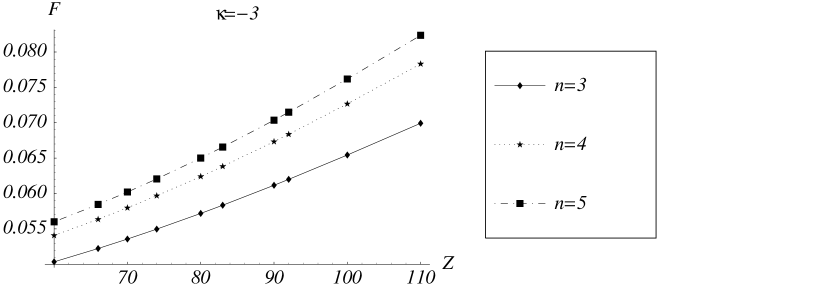
FIG. 1.: Scaled self-energy $F(Z\alpha)$ for $d_{5/2}$ states of levels $n=3$, 4 and 5.

FIG. 2.: Scaled self-energy $F(Z\alpha)$ for $f_{5/2}$ states of levels $n=4$ and 5.

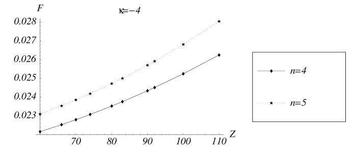
FIG. 3.: Scaled self-energy $F(Z\alpha)$ for $f_{7/2}$ states of levels $n$=4 and 5.

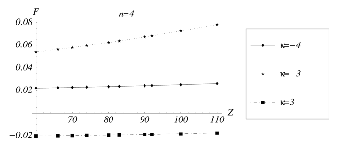
FIG. 4.: Scaled self-energy $F(Z\alpha)$ for atomic level $n=4$ and angular quantum numbers $\kappa=-3$, 3 and -4.

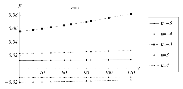
FIG. 5.: Scaled self-energy $F(Z\alpha)$ for atomic level $n=5$ and angular quantum numbers $\kappa$ such that $|\kappa|\geq 3$.