Large deformation of spherical vesicle studied by perturbation theory and Surface Evolver

Abstract

With tangent angle perturbation approach the axial symmetry deformation of a spherical vesicle in large under the pressure changes is studied by the elasticity theory of Helfrich spontaneous curvature model. Three main results in axial symmetry shape: biconcave shape, peanut shape, and one type of myelin are obtained. These axial symmetry morphology deformations are in agreement with those observed in lipsome experiments by dark-field light microscopy [Hotani, J. Mol. Biol. 178, 113 (1984)] and in the red blood cell with two thin filaments (myelin) observed in living state (see, Bessis, Living Blood Cells and Their Ultrastructure, Springer-Verlag, 1973). Furthermore, the biconcave shape and peanut shape can be simulated with the help of a powerful software, Surface Evolver [Brakke, Exp. Math. 1, 141 (1992)], in which the spontaneous curvature can be easy taken into account.

I introduction

Since the discovery of optical microscope, people have recognized that the human red blood cells (RBCs) [1] and lipsomes [2] can be in many beautiful and strange shapes depending on the environment in which they exist, such as pH value, osmotic pressure difference. The simplest model to explain these shapes is viewing RBC and lipsome as a vesicle of amphiphile bilayers.

For a long time, both the experimental and the theoretical aspects of amphiphile bilayers and monolayers have gathered much attention from physicists and chemists [3]. Helfrich has shown the importance of spontaneous curvature and has developed a phenomenological theory for the elasticity of fluid membranes by an analogy with the curvature elasticity of liquid crystals [4]. Many authors have studied the deformation of vesicles with different shapes among which the spherical vesicle plays a special role in these studies. The general shape equation of vesicles has been derived with differential geometry method [5], then some interesting numerical and analytical results have been reported [6, 7]. In the equation, the osmotic pressure difference between the external and internal sides of the vesicle membrane, especially the spontaneous curvature, and elastic modulus are important quantities. Among them, the influence of pressure on morphologic appearance of vesicle is the most important one to be considered. In shape study, RBC becomes an attractive model of vesicle in living cells. On the other hand, Hotani reported the lipsome shape transformation pathway when it was put in solution at certain concentration, and pointed out that osmotic pressure was found to be the driving force for the sequential transformations [2]. In the experiment the concentration changes slowly, and so does pressure, therefore, the shape formation of the lipsome can be seen as an equilibrium problem. In Hotani’s observation, single sphere finally formed and seemed to be stable forms because they showed no further morphological change. Jenkins and Peterson studied in detail the problem of the stability of RBC shapes [8], in which spherical vesicle was limit case. Ou-Yang and Helfrich studied instability and deformation of a spherical vesicle by pressure, and they found that any infinitesimal deformation corresponding to spherical harmonics $Y_{lm}$ would require a pressure difference larger than some threshold values [9]. The nonaxisymmetric deformation of RBC is investigated with a contour perturbation approach [10]. Obviously, the above approach is not able to deal with a large deformation of a vesicle shape , such as the myelin form in RBCs [1]. It then becomes a challenge to search for a method by which the large deformation of a spherical vesicle can be treated in theory of perturbation. In the present work we report an useful issue on solving the problem. The axial symmetry vesicle contour is expressed as $Z=-\int\tan\Psi d\rho$ where $\Psi$ is the tangent angle of the contour (see Fig. 1). One can find that a small change of $\Psi$ at $\Psi$ $\rightarrow$ $\pi/2$ is able to cause a large deformation in contour. Just like the method of Deuling and Helfrich [6], we introduce an alternative variable of $\sin\Psi$, $u$, thus, the contour Z will change with considerable amplitude as $\sin\Psi$ has small perturbation. with the issue we can calculate the large deformation of the contour via perturbation approach.

In this paper, we do some calculations about the large deformation of a spherical vesicle with the new approach via pressure perturbation, varied biconcave shapes and one kind of peanut shape can be obtained. Especially we show one type of myelin form with two long filaments attaching on the spherical vesicle. To confirm the analytic calculation we also perform some computer simulations with the help of a powerful software, Surface Evolver [11].

II perturbation theory

Equilibrium shapes of phospholipid vesicles are assumed to correspond to the local minima of the elastic free energy of these systems. In the Helfrich spontaneous curvature model, the spontaneous curvature plays a fundamental role in accounting for the different morphologic appearances of vesicles [4]. According to Helfrich’s theory, the free energy of a vesicle is written as

$$F=\frac{1}{2}k_{c}\oint(c_{1}+c_{2}-c_{0})^{2}dA+\Delta p\int dV+\lambda\oint dA,$$ (1)

where $k_{c}$ is the bending elastic modulus; $c_{1}$ and $c_{2}$ are the two principle curvatures of the surface of the vesicle, $c_{0}$ is the spontaneous curvature to describe the possible asymmetry of the outer and inner layers of membrane, and dA and dV are the surface area and the volume elements for the vesicle, respectively. The Lagrange Multipliers $\Delta p$ and $\lambda$ take account of the constraints of constant volume and area, respectively, and can be physically understood as the pressure difference between the external and the internal environment and the surface tensile coefficient. The general shape equation has been derived via variational calculus [5] to be

$$\Delta p-2\lambda H+k_{c}(2H+c_{0})(2H^{2}-2K-c_{0}H)+2k_{c}\bigtriangledown^{2}H$$ (3)

$$=0,$$

where $H$ and $K$ are the mean and the Gaussian curvatures, respectively, and $\bigtriangledown^{2}$ is the Laplace-Beltrami operator [9]. Assuming that the shape has axial symmetry, the general shape equation becomes a third order nonlinear differential equation

$$\cos^{3} \Psi\frac{d^{3}\Psi}{d\rho^{3}}=4\sin\Psi\cos^{2}\Psi\frac{d^{2}\Psi}{d\rho^{2}}\frac{d\Psi}{d\rho}$$ (9)

$$-\cos\Psi(\sin^{2}\Psi-\frac{1}{2}\cos^{2}\Psi)(\frac{d\Psi}{d\rho})^{3}$$

$$+7\frac{\sin\Psi\cos^{2}\Psi}{2\rho}(\frac{d\Psi}{d\rho})^{2}-\frac{2\cos^{3}\Psi}{\rho}(\frac{d^{2}\Psi}{d\rho^{2}})$$

$$+\left[\frac{c_{0}^{2}}{2}-\frac{2c_{0}\sin\Psi}{\rho}+\frac{\lambda}{k_{c}}-\frac{\sin^{2}\Psi-2\cos^{2}\Psi}{2\rho^{2}}\right]\times$$

$$\cos\Psi\frac{d\Psi}{d\rho}+\left[\frac{\Delta p}{k_{c}}+\frac{\lambda\sin\Psi}{k_{c}\rho}\right.$$

$$\left.+\frac{c_{0}^{2}\sin\Psi}{2\rho}-\frac{\sin^{3}\Psi+2\sin\Psi\cos^{2}\Psi}{2\rho^{3}}\right],$$

where $\rho$ is the distance from the symmetric $Z$ axis of rotation, $\Psi(\rho)$ is the angle made by the rotational axis and the surface normal of the vesicle, also the tangent angle of the contour $Z(\rho)$ (see Fig. 1). Let $\sin\Psi=u$, $\rho=x$ [12], the equation takes the following form

$$\frac{\Delta p}{k_{c}}+[\frac{1}{x^{3}}-\frac{1}{x}\left(\frac{\lambda}{k_{c}}+\frac{c_{0}^{2}}{2}\right)]u-\frac{u^{3}}{2x^{3}}-\left(\frac{1}{x^{2}}+\frac{\lambda}{k_{c}}+\frac{c_{0}^{2}}{2}\right)u^{\prime}$$ (10)

$$+\frac{3}{2}\frac{u^{2}u^{\prime}}{x^{2}}-\frac{3uu^{\prime 2}}{2x}+\frac{2c_{0}uu^{\prime}}{x}+\frac{u^{\prime 3}}{2}+\frac{2(1-u^{2})u^{\prime\prime}}{x}$$ (11)

$$-uu^{\prime}u^{\prime\prime}+(1-u^{2})u^{\prime\prime\prime}=0,$$ (12)

where prime means derivative of $u(x)$ with respect to x. It is obvious that a sphere with radius $r_{0}$ is always a solution of Eq. (12) ($u=x/r_{0}$), and its pressure difference $\Delta p\equiv\Delta p_{0}$ must obey

$$\Delta p_{0}r_{0}^{3}-2\lambda r_{0}^{2}+k_{c}c_{0}r_{0}(2-c_{0}r_{0})=0.$$ (13)

Jenkins [8], Ou-Yang and Helfrich [5] have studied the stability of the spherical vesicles. Now we calculate the first order pressure perturbation contribution to $u$ using the Eq. (12). When the pressure difference $\Delta p$ is slightly deviated from its equilibrium value $\Delta p_{0}$, i.e. , $\Delta p=\Delta p_{0}+\delta\Delta p$, Eq. (13) is no longer satisfied, what will be the shape of the vesicle? Here we give an answer to this question with our detailed calculation.

By expanding $u$ as $u=u_{0}+u_{1}+u_{2}+...$ with $u_{1}\sim\delta\Delta p$, $u_{2}\sim(\delta\Delta p)^{2}$, … , while $u_{0}$ takes $x/r_{0}$, we find $u_{1}$ to satisfy the following linear third-order differential equation

$$\left(1-\frac{x^{2}}{r_{0}^{2}}\right)u_{1}^{\prime\prime\prime}+\left(\frac{2}{x}-\frac{3x}{r_{0}^{2}}\right)u_{1}^{\prime\prime}$$ (14)

$$-\left(\frac{1}{x^{2}}+\frac{\lambda}{k_{c}}+\frac{c_{0}^{2}}{2}-\frac{2c_{0}}{r_{0}}\right)u_{1}^{\prime}$$ (15)

$$+\left[\frac{1}{x^{3}}-\frac{1}{x}\left(\frac{\lambda}{k_{c}}+\frac{c_{0}^{2}}{2}+\frac{2c_{0}}{r_{0}}\right)\right]u_{1}+\frac{\delta\Delta p}{k_{c}}=0,$$ (16)

where $\delta\Delta p$ is the pressure perturbation. After introducing a new variable $\xi=x/r_{0}$, i.e., $u_{0}$ takes $\xi$, the above perturbation equation becomes

$$( 1-\xi^{2})u_{1}^{\prime\prime\prime}+(\frac{2}{\xi}-3\xi)u_{1}^{\prime\prime}-(\frac{1}{\xi^{2}}+b)u_{1}^{\prime}$$ (18)

$$+(\frac{1}{\xi^{3}}-\frac{b}{\xi})u_{1}+p=0,$$

where two dimensionless parameters are: $b\equiv r_{0}^{2}\lambda/k_{c}+c_{0}^{2}r_{0}^{2}/2-2c_{0}r_{0}$, $p\equiv r_{0}^{3}\delta\Delta p/k_{c}$, and now prime means derivative of $u(\xi)$ with respect to $\xi$. It is obvious that $u_{1}=(p/2b)\xi$ is a particular solution. Here we suppose that $b\neq 0$. For the case of $b=0$, we discuss it in the next section. Then the first step for solving Eq. (18) is to solve the following homogeneous equation

$$( 1-\xi^{2})u_{1}^{\prime\prime\prime}+(\frac{2}{\xi}-3\xi)u_{1}^{\prime\prime}-(\frac{1}{\xi^{2}}+b)u_{1}^{\prime}$$ (20)

$$+\left(\frac{1}{\xi^{3}}-\frac{b}{\xi}\right)u_{1}=0.$$

It is lucky that $u_{1}=\xi^{-1}$ is a particular solution of this homogeneous equation. We denote it as $u_{10}=\xi^{-1}$, and let [13]

$$u_{1}=\frac{1}{\xi}\int z(\xi)d\xi,$$ (21)

Eq. (20) is thus reduced into the following second-order homogeneous differential equation

$$\xi^{2}(1-\xi^{2})z^{\prime\prime}-\xi z^{\prime}+(1-b\xi^{2})z=0.$$ (22)

To solve it, we refer to the following standard form of the equation [14]

$$x^{2}(ax^{n}-1)y_{xx}^{{}^{\prime\prime}}+x(atx^{n}+q)y_{x}^{{}^{\prime}}+(arx^{n}+s)y=0.$$ (23)

There are four roots $A_{1}$, $A_{2}$ and $B_{1}$, $B_{2}$ of the quadratic equations: $A^{2}-(q+1)A-s=0$ and $B^{2}-(t-1)B+r=0$. Then four parameters c, $\alpha$, $\beta$, and $\gamma$ can be defined by the relations: $c=A_{1}$, $\alpha=\frac{A_{1}+B_{1}}{n}$, $\beta=\frac{A_{1}+B_{2}}{n}$, $\gamma=\frac{A_{1}-A_{2}}{n}+1$ and the solution of the standard equation has the form $y=x^{c}\omega(ax^{n})$, where $\omega(\xi)$ is the general solution of the hypergeometric equation

$$\xi(\xi-1)\omega_{\xi\xi}^{{}^{\prime\prime}}+[(\alpha+\beta+1)-\gamma]\omega_{\xi}^{{}^{\prime}}+\alpha\beta\omega=0.$$ (24)

In the case of Eq. (22), we have $a=1$, $n=2$, $t=0$, $q=1$, $r=b$ and $s=-1$. Two quadratic algebra equations associated with Eq. (22) are introduced: $A^{2}-2A+1=0$ and $B^{2}+B+b=0$. Their roots are: $A_{1}=A_{2}=1$, and $B_{1}$, $B_{2}=(-1\pm\sqrt{1-4b})/2$. From them three characterized numbers can be calculated :

$$\alpha = \frac{A_{1}+B_{1}}{2}=\frac{1+\sqrt{1-4b}}{4},$$ (25)

$$\beta = \frac{A_{1}+B_{2}}{2}=\frac{1-\sqrt{1-4b}}{4},$$ (26)

$$\gamma = 1.$$ (27)

Then we have

$$z(\xi)=\xi\omega(\xi^{2}),$$ (28)

where $\omega(\eta)$, $\eta\equiv\xi^{2}$, is the solution of Gauss hypergeometric equation:

$$\eta(\eta-1)\omega^{\prime\prime}+[(\alpha+\beta+1)\eta-\gamma]\omega^{\prime}+\alpha\beta\omega=0.$$ (29)

At once, let its solution $\omega_{1}$ take the hypergeometric function [14] as

$$\omega_{1}=F(\alpha,\beta,\gamma,\eta).$$ (30)

Because $\gamma=1$ is an integral, we have the second solution of Eq. (29) [15]

$$\omega_{2}(\eta) = F(\alpha,\beta,\gamma,\eta)\ln(\eta)$$ (33)

$$+\sum_{k=0}^{\infty}\frac{(\alpha)_{k}(\beta)_{k}}{(k!)^{2}}\eta^{k}\{\phi(\alpha+k)$$

$$+\phi(\beta+k)-2\phi(1+k)\},$$

where $(\lambda)_{0}=1$, $(\lambda)_{n}=\lambda(\lambda+1)...(\lambda+n-1)=\frac{\Gamma(\lambda+n)}{\Gamma(\lambda)}$, $(n\geq 1)$, $\phi(\tau)=\frac{d\ln(\Gamma(\tau))}{d\tau}$, and $\Gamma(\tau)$ is Euler Gamma function. Finally, we find two solutions of Eq. (22)

$$z_{1} = \xi\omega_{1}(\eta)=\xi\omega_{1}(\xi^{2})=\xi F(\alpha,\beta,1,\xi^{2}),$$ (34)

$$z_{2} = \xi\omega_{2}(\eta)=\xi\omega_{2}(\xi^{2})=\xi F(\alpha,\beta,1,\xi^{2})\ln\xi^{2}+$$ (37)

$$\sum_{k=0}^{\infty}\frac{(\alpha)_{k}(\beta)_{k}}{(k!)^{2}}\eta^{2k+1}\{\phi(\alpha+k)$$

$$+\phi(\beta+k)-2\phi(1+k)\},$$

and two solutions of Eq. (20) $u_{11}=\frac{1}{2\xi}\int\omega_{1}(\xi^{2})d\xi^{2}$, $u_{12}=\frac{1}{2\xi}\int\omega_{2}(\xi^{2})d\xi^{2}$. To obtain the detailed forms of $u_{11}$ and $u_{12}$ two integrals, $\int F(\alpha,\beta,\gamma,\eta)d\eta$ and $\int F(\alpha,\beta,\gamma,\eta)\ln\eta d\eta$, need to calculate. We have (see the details in appendix)

$$\int F(\alpha,\beta,\gamma,\eta)d\eta$$ (38)

$$=\frac{1}{\alpha+\beta-\alpha\beta-1}F(\alpha,\beta,\gamma,\eta)\left[(\alpha+\beta-1)\eta+1-\gamma\right]$$ (39)

$$+\eta(\eta-1)F^{\prime}(\alpha,\beta,\gamma,\eta),$$ (40)

and, due to $\alpha+\beta-\alpha\beta-1\neq 0$ and $\gamma=1$,

$$\int \ln\eta F(\alpha,\beta,\gamma,\eta)d\eta$$ (45)

$$=\frac{1}{\alpha+\beta-\alpha\beta-1}\{F^{\prime}(\alpha,\beta,\gamma,\eta)\eta(\eta-1)\ln\eta$$

$$+(\alpha+\beta-1)\eta F(\alpha,\beta,1,\eta)\ln\eta+(1-\eta)F(\alpha,\beta,1,\eta)\}$$

$$+\frac{2-\alpha-\beta}{(\alpha+\beta-\alpha\beta-1)^{2}}\{\eta F(\alpha,\beta,1,\eta)(\alpha+\beta-1)$$

$$+\eta(\eta-1)F^{\prime}(\alpha,\beta,1,\eta)\},$$

where $F^{\prime}(\alpha,\beta,1,\eta)=\frac{d}{d\eta}F(\alpha,\beta,1,\eta)=\alpha\beta F(\alpha+1,\beta+1,2,\eta)$. Now, we can write down three independent solutions of Eq. (20):

$$u_{10} = \frac{1}{\xi},$$ (46)

$$u_{11} = \frac{1}{\xi}\int\xi F(\alpha,\beta,1,\xi^{2})d\xi$$ (47)

$$= \frac{1}{2\xi(\alpha+\beta-\alpha\beta-1)}\{F(\alpha,\beta,1,\xi^{2})(\alpha+\beta-1)\xi^{2}$$ (49)

$$+\xi^{2}(\xi^{2}-1)\alpha\beta F(\alpha+1,\beta+1,2,\xi^{2})\},$$

$$u_{12} = \frac{1}{\xi}\int\xi\ln\xi F(\alpha,\beta,\gamma,\xi^{2})d\xi$$ (52)

$$+\frac{1}{\xi}\int\sum_{k=0}^{\infty}\frac{(\alpha)_{k}(\beta)_{k}}{(k!)^{2}}\xi^{2k+1}\{\phi(\alpha+k)$$

$$+\phi(\beta+k)-2\phi(1+k)\}d\xi$$

$$= \frac{1}{2\xi}\{\frac{1}{\alpha+\beta-\alpha\beta-1}$$ (60)

$$[\alpha\beta F(\alpha+1,\beta+1,2,\xi^{2})\xi^{2}(\xi^{2}-1)\ln\xi^{2}$$

$$+(\alpha+\beta-1)\xi^{2}F(\alpha,\beta,1,\xi^{2})\ln\xi^{2}+$$

$$(1-\xi^{2})F(\alpha,\beta,1,\xi^{2})]+\frac{2-\alpha-\beta}{(\alpha+\beta-\alpha\beta-1)^{2}}\times$$

$$[\xi^{2}F(\alpha,\beta,1,\xi^{2})(\alpha+\beta-1)$$

$$+\xi^{2}(\xi^{2}-1)\alpha\beta F(\alpha+1,\beta+1,2,\xi^{2})]\}$$

$$+\sum_{k=0}^{\infty}\frac{(\alpha)_{k}(\beta)_{k}}{(k!)^{2}}\xi^{2k+1}\{\phi(\alpha+k)+\phi(\beta+k)$$

$$-2\phi(1+k)\}.$$

From Eq. (18), Eq. (20) and Eq. (60) we get the general solution of Eq. (12) as

$$u=u_{0}+pc_{10}\frac{1}{\xi}+pc_{11}u_{11}+pc_{12}u_{12}+p\frac{1}{2b}\xi,$$ (61)

where $c_{10}$, $c_{11}$, and $c_{12}$ are three integral constants.

In general, the hypergeometric function can be expressed as the series

$$F(\alpha,\beta,\gamma,\eta)=1+\sum_{k=0}^{\infty}\frac{(\alpha)_{k}(\beta)_{k}}{(\gamma)_{k}}\frac{\eta^{k}}{k!},$$ (62)

where $(\lambda)_{0}=1,(\lambda)_{n}=\lambda(\lambda+1)...(\lambda+n-1)$. $F(\alpha,\beta,\gamma,\eta)$ is a fortiori convergent for $|\eta|<1$. In the present case $\gamma=1$, $\alpha=(1+\sqrt{1-4b})/4$ and $\beta=(1-\sqrt{1-4b})/4$, the condition $Re(\gamma-\alpha-\beta)=\frac{1}{2}>0$ is satisfied, so $F(\alpha,\beta,1,\eta)$ is conditional convergent while $\eta=1$, and $F(\alpha,\beta,\gamma,1)=\frac{\Gamma(\gamma)\Gamma(\gamma-\alpha-\beta)}{\Gamma(\gamma-\alpha)\Gamma(\gamma-\beta)}$. But this case is not true to $F(\alpha+1,\beta+1,2,\eta)$ when $\eta=1$, and the analytical continuation for it gives the complex result. So we limit our discussion within $0\leq\xi<1$ to avoid the divergence and imaginary number. From another point of view, if we consider that $\xi$ can be or be more than unit, that three integral constants $c_{10}$, $c_{11}$ and $c_{12}$ in Eq. (60) must be zero, so the solution of Eq. (12) will be $u_{0}$ (sphere solution) adding that particular one, i.e.,

$$u=u_{0}+\frac{p}{2b}\xi,$$ (63)

the sphere still keeps its shape under a pressure perturbation varying its size only. After obtaining the total solution of Eq. (16), using the integration

$$Z=-\int\tan\Psi d\rho,$$ (64)

we can give the contour of the axial symmetry shape of vesicle with deformation. Our numerical calculation about Gauss hypergeometric function is worked out with the famous software, Mathematica. In the following sections some cases are shown for details.

III special case

First we discuss the special case of $b=0$ in the Eq. (18). That is to solve the following equation

$$(1-\xi^{2})u^{\prime\prime\prime}+(\frac{2}{\xi}-3\xi)u^{\prime\prime}-\frac{1}{\xi^{2}}u^{\prime}+\frac{1}{\xi^{3}}u+p=0.$$ (65)

It is convenient to check that $u=p/2\xi\log{\xi}$ is a particular solution. So the task remained is to solve the associated homogeneous third order equation

$$(1-\xi^{2})u^{\prime\prime\prime}+(\frac{2}{\xi}-3\xi)u^{\prime\prime}-\frac{1}{\xi^{2}}u^{\prime}+\frac{1}{\xi^{3}}u=0.$$ (66)

It is easy to verify that $u_{1}=\xi$, $u_{2}=1/\xi$ are two independent solutions. According to the handbook [14], the general solution of Eq. (66) is written as

$$u=c_{1}u_{10}+c_{2}u_{2}+c_{3}(u_{2}\int{u_{1}\theta dx}-u_{1}\int{u_{2}\theta dx})$$ (67)

where

$$\theta=\exp[\int(f_{2}/f_{3})dx](u_{1}u_{2}^{\prime}-u_{1}^{\prime}u_{2})^{-2},$$ (68)

$$f_{2}=2/\xi-3\xi,\quad and\quad f_{3}=1-\xi^{2}.$$ (69)

The final result is

$$u = \xi+c_{1}\xi+\frac{c_{2}}{\xi}+c_{3}(\xi\log{\frac{1+\sqrt{1-\xi^{2}}}{\xi}})$$ (71)

$$+\frac{p}{2}\xi\log{\xi}.$$

If   $c_{2}=c_{3}=0$, we have

$$u=\xi+c_{1}\xi+\frac{p}{2}\xi\log{\xi}.$$ (72)

Eq. (72) satisfies the general shape equation Eq. (12). It can give the biconcave shape [7] and many interesting shapes described as have been shown in [16].

IV Biconcave and peanut shape

With the help of microscopes people have made detailed observation of RBC which can assume various shapes [1]. Generally, RBC takes biconcave disk shape (in blood capillary it has very large deformation [17]), while some pathologic cells take other abnormality (such as in sickle cell disease). If RBC is subjected to different environment, various pH values for example, it will make some considerable deformations, such as, Cup (Stomatocyte), Bell (Codocyte), Sea urchin (Echinocyte) et al.. Moreover, beginning with biconcave lipsome vesicle Hotani present many beautiful transformations among which the peanut shape was included [2]. Surely the biconcave shape attracts many attention. In this section we use the general theory of the section II to show that spherical vesicle can transform into biconcave shape via pressure perturbation. Because $\Psi=0$ at $\rho=0$ and $\Psi=\pi/2$ at $\rho=\rho_{m}$ (see Fig. 1), there are two boundary conditions at $\rho=0$ and $\rho=\rho_{m}$, i.e., $\xi=0$ and $\xi=\xi_{m}$

$$u|_{\xi=0}=0;\qquad\qquad u|_{\xi=\xi_{m}}=1,$$ (73)

where $\xi_{m}=\rho_{m}/r_{0}$. Thus there are two relations between the three coefficients $c_{10}$, $c_{11}$ and $c_{12}$ as

$$c_{10} = \frac{-c_{12}}{2(\alpha+\beta-\alpha\beta-1)},$$ (74)

$$c_{11} = \{c_{12}\{\frac{2-\alpha-\beta}{(\alpha+\beta-\alpha\beta-1)}\frac{1}{2(\alpha+\beta-\alpha\beta-1)}\times$$ (77)

$$\frac{\Gamma(\gamma)\Gamma(\gamma-\alpha-\beta)}{\Gamma(\gamma-\alpha)\Gamma(\gamma-\beta)}-\frac{1}{2(\alpha+\beta-\alpha\beta-1)}\}+\frac{1}{2b}\}\times$$

$$\frac{2(\alpha+\beta-\alpha\beta-1)\Gamma(\gamma-\alpha)\Gamma(\gamma-\beta)}{\Gamma(\gamma)\Gamma(\gamma-\alpha-\beta)(\alpha+\beta-1)}.$$

So far, in the above solution there is still one relation to be determined. We can calculate it via using the conservation of area of sphere. For a rotational surface the area element can be expressed as

$$ds = 2\pi x(1-u^{2})^{-1/2}dx.$$ (79)

Using reduced dimensionless area $s_{r}$ defined by $ds=4\pi r_{0}^{2}ds_{r}$, we have $ds_{r}=\frac{1}{2}\xi(1-u^{2})^{-1/2}d\xi$, and another boundary condition to take account of the area conservation

$$\int_{0}^{\xi_{m}}\xi(1-u^{2})^{-1/2}d\xi=1.$$ (80)

Basing on Eq. (61), Eq. (LABEL:29) and Eq. (80), the values of $c_{10}$, $c_{11}$ and $c_{12}$ can be fixed completely. So the shape is also determined with Eq. (64). But in practical computation the value of $\xi_{m}$ in Eq. (80) can not be directly predicted. Therefore, in our computation, we treat it as a free boundary problem, i.e., we let $\xi_{m}$ takes a series of value, correspondingly, a series of deformation of the original spherical vesicle and their total energy can be calculated [18]. The less total energy, the easier the deformation can be observed in practice (experiments). From the Eq. (61) the different shapes can be got via Eq. (64). We show our numerical results in Fig. 3, Fig. 9 and Fig. 12. In fact, in Fig. 3 only the top right quadrant contours of vesicle are shown. In order to obtain the total vesicle surface two operations need to be done in succession: at first, rotate it with the $Z$ axis, this give the upper part of the surface; second, take mirror reflection. In order to describe the parameters corresponding to the curves in Figs. 3-6, we define a new parameter $v$ as $v$ $\equiv$ $V/V_{0}$ where $V$ is the volume of vesicle and $V_{0}$ is the volume of original spherical vesicle. The pressure corresponding to each curve is defined as $\frac{\Delta p-\Delta p_{0}}{\Delta p_{0}}$, $\Delta p$ is the pressure related to the deformed vesicle while $\Delta p_{0}$ is the pressure difference of the original spherical vesicle. The shapes given in Fig. 3 are obtained at the constant spontaneous curvature and surface tension, i.e., $c_{0}r_{0}$ =-2.4 and $\lambda r_{0}^{2}/k_{c}=0.01$. The values of ($\frac{\Delta p-\Delta p_{0}}{\Delta p_{0}}$, $v$) are calculated as ($-10^{-6}$, 0.99), (0.01, 0.3), (0.01, 0.5), (0.05, 0.3), (0.01, 0.62) for curves 2-6, respectively. The curve 1 is the initial shape of sphere. Two three-dimensional shapes of biconcave and peanut are shown in Fig. 9 and Fig. 12, respectively. In principle, energy corresponding to every curve can be calculated with the formula in [18]. The above calculated biconcave shape can be simulated on the basis of the elasticity theory of Helfrich spontaneous curvature model by Surface Evolver [11]. The simulated results, corresponding to biconcave and peanut shape, are shown in Fig. 13 and Fig. 16, respectively, in which the $A/A_{0}$ gives the ratio of surface area of vesicle to that of the initial spherical vesicle. Both they are observed in blood cell [1] and lipsome vesicles [2]. Furthermore, We turn to analysis the behavior of deformation near rotational axis. After obtaining the general solution Eq. (61), the behavior of deformation near the rotational axis can be got by expanding it to first order of $p$ as

$$u = \xi+\frac{1}{2}pc_{11}\xi+pc_{12}(\ln\xi+\frac{1}{2}+\frac{\frac{1}{2}\alpha\beta}{\alpha+\beta-\alpha\beta-1})\xi+\frac{p}{2b}\xi$$ (81)

$$= A\xi+B\xi\ln\xi.$$ (82)

This equation describes the shape near polar points, and the equation is very similar to the biconcave shape of red blood cell [7]. In this equation there is no any singular point in the region $0\leq\xi<1$.

V Myelin form

Myelin form may originate from all blood cells [1]. Shadowing technique in microscopy reveals that myelin forms are hollow structures. When a RBC is in aging, aged and damaged states, it gives rise to large myelin forms which may take various types: filaments, beads or strings of beads. These filaments, which are easily seen with phase contrast microscopy, may remain attached to the surface of the RBC at one end. Here we choose the so called Delaunay’s surface solution [7] from the general solution of the perturbation Eq. (16), which can give a type of myelin form generating from the vesicle. In the book of Bessis [1], there is a photo of this kind of Medusa head. Now let us first discuss the general solution Eq. (61) in the case of $c_{11}=c_{12}=0$:

$$u=(1+\frac{p}{2b})\xi+c_{10}/\xi.$$ (83)

Substituting it into the general shape equation Eq. (12) yields two relations: $1+p/2b=c_{0}r_{0}/2$, and $\Delta p=c_{0}\lambda$. It should be noticed that $\Delta p=\Delta p_{0}+p$. $\Delta p_{0}$ can be solved from Eq. (13), then we find

$$p=(2c_{0}-c_{0}^{2}r_{0})r_{0}-\frac{2\lambda r_{0}^{2}}{k_{c}}+\frac{c_{0}\lambda r_{0}^{3}}{k_{c}}.$$ (84)

Considering the mentioned relation $1+p/2b=c_{0}r_{0}$ we have

$$(c_{0}^{2}r_{0}-2c_{0})r_{0}+\frac{2\lambda r_{0}^{2}}{k_{c}}-\frac{c_{0}\lambda r_{0}^{3}}{k_{c}}=2b-c_{0}r_{0}b.$$ (85)

The value of $c_{10}$ in Eq. (83) can be determined via boundary condition: $u|_{\xi=\xi_{m}}=1$ ($\xi=\xi_{m}$, $\Psi=\pi/2$). It leads to $c_{10}=(\xi_{m}-(1+\frac{p}{2b})\xi_{m}^{2})$ and finally we obtained from Eq. (83) the Delaunay’s solution

$$u=\frac{c_{0}r_{0}}{2}\xi+\frac{\xi_{m}-c_{0}r_{0}\xi_{m}^{2}/2}{\xi}.$$ (86)

With different $c_{0}r_{0}$ and $\xi_{m}$, the various contours can be numerically calculated using Eq. (64) (see Fig. 18 and Fig. 20). Not total length of filament is drawn in this two figures. In fact, those filaments are swollen distally and our present calculation can not give an exact description yet.

VI conclusions and discussions

Now we give here our main conclusions as what follows: With tangent angle perturbation approach, we can calculate the large deformation of spherical vesicle under pressure perturbation. From the general perturbation solutions, the biconcave and peanut shapes can be obtained and a kind of myelin form is shown to be existed. Our all calculations are based on the elasticity theory of Helfrich spontaneous curvature model and it does give good accordance with some complex shapes of lipsome vesicles (see photographs in [2]) and RBCs (see photographs in [1]) with computer simulation [19, 1, 2].

two integrals relating to Gauss hypergeometric function

In the appendix we give the derivation of two relating integral about Gauss hypergeometric function. The main idea and method are to use hypergeometric equation itself. From the hypergeometric equation Eq. (29)

$$x~{}(1-x)\omega^{\prime\prime}+\left[\gamma-~{}(\alpha+\beta+1)x\right]\omega^{\prime}-\alpha\beta\omega=0,$$ (87)

we have

$$\omega=\frac{1}{\alpha\beta}x~{}(1-x)\omega^{\prime\prime}+\left[\gamma-~{}(\alpha+\beta+1)\right]\omega^{\prime},$$ (88)

and

$$\int\omega dx=\frac{x~{}(1-x)\omega^{\prime}}{1-\alpha-\beta+\alpha\beta}+\frac{\gamma-1+~{}(\alpha+\beta+1)x}{1-\alpha-\beta+\alpha\beta}\omega.$$ (89)

Using the same method and with the key point $\gamma=1$, through a lengthy derivation, we obtain

$$\int\ln x\omega dx = \frac{1}{\alpha+\beta+1}\times$$ (93)

$$[\omega^{\prime}x~{}(x-1)\ln x+~{}(\alpha+\beta-1)x\omega\ln x$$

$$+(1-x)\omega]+\frac{2-\alpha-\beta}{\left(\alpha+\beta-\alpha\beta-1\right)^{2}}\times$$

$$[x\omega~{}(\alpha+\beta-1)+x(x-1)\omega^{\prime}].$$

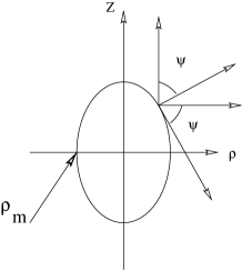
FIG. 1.: Convection of angle $\Psi$ for the contour of axial symmetry vesicle. At the north pole the $\Psi$ value takes zero. $\rho_{m}$ gives the boundary position of $\rho$.

FIG. 2.: The numerical results from the solution of Eq. (61). Only the top right quadrant contours are shown. Curve 1 corresponds to spherical vesicle, while curves 2-6 show much swelling or oblate biconcave shapes. The energy of each vesicle can be calculated with the formula given in [18].

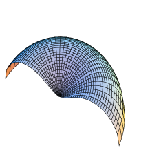
FIG. 3.: Biconcave shape in three-dimensional (half of upper part is shown) with $\xi_{m}=0.9999$, $v=0.1$ (the ratio of volume of the deformed vesicle to that of the initial sphere), $\lambda r_{0}^{2}/k_{c}=0.01$, $c_{0}r_{0}=-3.0$. When the parameters are adjusted, the other biconcave shapes can be formed, much oblate or much swelling (see, Fig. 3).

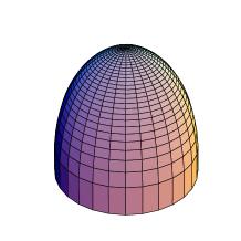
FIG. 4.: Numerical result of upper-half peanut shape in three-dimensional with $\xi_{m}=0.8$, $v=0.4$, $\lambda r_{0}^{2}/k_{c}=0.01$, and $c_{0}r_{0}=0.01$.

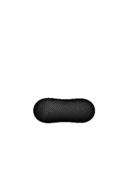
FIG. 5.: Biconcave shape in three-dimensional simulated with Surface Evolver. The parameters take $H_{0}$=-1.38, $k_{c}$=1, $A/A_{0}$=0.96 (the ratio of surface area of vesicle and that of the initial sphere), $v$=0.92, and $\lambda r_{0}^{2}/k_{c}$=0.48.

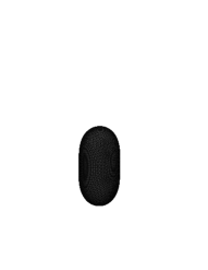
FIG. 6.: Peanut shape in three-dimensional simulated with Surface Evolver. The using parameters are $c_{0}r_{0}$=1.38, $k_{c}$=1, $A/A_{0}$=0.83 (the ratio between surface area of vesicle and that of the initial sphere), $v$=0.79, and $\lambda r_{0}^{2}/k_{c}$=0.48.

FIG. 7.: The numerical results corresponding to Eq. (65). Only the top right quadrant contours are shown. The parameters corresponds to curve 4 (contour in Fig. 20) are: $c_{0}r_{0}=2$, $\xi_{m}=0.9$.

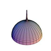
FIG. 8.: The calculated shape of upper-half of the myelin form of spherical vesicle in three-dimensional with $c_{0}r_{0}=2$, and $\xi_{m}=0.9$.

REFERENCES

- [1] M. Bessis, Living Blood Cells and Their Ultrastructure (Springer-Verlag, Berlin, 1973) (translated by Robert I. Weed); M. Bessis, et. al., Red Cell Shape, Physiology. Pathology. Ultrastructure (Springer-Verlag, New York, 1973).
- [2] H. Hotani, J. Mol. Biol. 178, 113 (1984).
- [3] For review, see (a) R. Lipowsky, Nature 349, 475 (1991); (b) Physics of Amphiphile Layers, edited by J. Meunier, D. Langeran and N. Boccara (Springer, Berlin, 1987); (c) Statistical Mechanics of Membranes and Surfaces, Ed. by D. Nelson et. al. (World Scientific, Singapore, 1989).
- [4] W. Helfrich, Z. Naturforch. 28C, 693 (1973).
- [5] Z.-C. Ou-Yang and W. Helfrich, Phys. Rev. Lett. 59, 2486 (1987).
- [6] H. J. Deuling and W. Helfrich, Biophys. J. 16, 861 (1976); L. Miao, B. Fourcade, M. Rao, and M. Wortis, Phys. Rev. A 43, 6843 (1991); U. Seifert, K. Berndl, and R. Lipowsky, Phys. Rev. A 41, 1182 (1991).
- [7] H. Naito, M. Okuda and Ou-Yang Zhong-can, Phys. Rev. E 48, 2304 (1993); Phys. Rev. Lett. 74, 4345 (1995).
- [8] J. T. Jenkins, J. Math. Biol. 4, 149 (1977); M. A. Peterson, J. Math. Phys. 26, 711 (1985); J. Appl. Phys. 57, 1739 (1985); Mol. Cryst. Liq. Cryst. 127, 159 (1985); ibid. 127, 257 (1985).
- [9] Ou-Yang Zhong-can and W. Helfrich, Phys. Rev. A 39, 5280 (1989).
- [10] H. Naito, M. Okuda and Z.-C. Ou-Yang , Phys. Rew. E 54, 2816 (1996); Q. Liu, J. Yan and Z.-C. Ou-Yang, Phys. Lett. A 260, 162 (1999).
- [11] K. Brakke, Exp. Math. 1, 141 (1992).
- [12] W. Zheng and Ou-Yang Zhong-can, Commun. Theor. Phys. 15, 505 (1991).
- [13] G. M. Murphy, Ordinary Differential Equations and Their Solutions (D. Van Nostrand Company, New York, 1960).
- [14] Andrei D. Polyanin, Valentin F. Zaitsev, Handbook of exact solutions for ordinary differential equations (CRC Press, Boca Raton, 1995).
- [15] E. T. Whittaker and G. N. Watson, Modern Analysis (Cambridge, 1927).
- [16] Q. Liu et al., Phys. Rev. E 60, 3227 (1999).
- [17] P.I. Brnemark and J. Lindstrm, Biorheology, 1, 139 (1963).
- [18] From , when keeps constant, the total energy is derived as . In the calculations this expression is expanded to first order of , and is considered.
- [19] J. Yan et al., Phys. Rev. E 58, 4730 (1998); other simulations from the Surface Evolver are in preparation.