Information-theoretic approach to the study of control systems

Abstract

We propose an information-theoretic framework for analyzing control systems based on the close relationship of controllers to communication channels. A communication channel takes an input state and transforms it into an output state. A controller, similarly, takes the initial state of a system to be controlled and transforms it into a target state. In this sense, a controller can be thought of as an actuation channel that acts on inputs to produce desired outputs. In this transformation process, two different control strategies can be adopted: (i) the controller applies an actuation dynamics that is independent of the state of the system to be controlled (open-loop control); or (ii) the controller enacts an actuation dynamics that is based on some information about the state of the controlled system (closed-loop control). Using this communication channel model of control, we provide necessary and sufficient conditions for a system to be perfectly controllable and perfectly observable in terms of information and entropy. In addition, we derive a quantitative trade-off between the amount of information gathered by a closed-loop controller and its relative performance advantage over an open-loop controller in stabilizing a system. This work supplements earlier results [H. Touchette, S. Lloyd, Phys. Rev. Lett. 84, 1156 (2000)] by providing new derivations of the advantage afforded by closed-loop control and by proposing an information-based optimality criterion for control systems. New applications of this approach pertaining to proportional controllers, and the control of chaotic maps are also presented.

I Introduction

It is common in studying controllers to describe the interplay between the sensors which estimate the state of a system intended to be controlled, and the actuators used to actually modify the dynamics of the controlled system as a transfer of information involving three steps: estimation, decision, and actuation. In the first step, sensors are used to gather information from the controlled system in the form of data relative to its state (estimation step). This information is then processed according to some plan or control strategy in order to determine which control dynamics is to be applied (decision step), to be finally transferred to the actuators which feed the processed information back to the controlled system to modify its dynamics, typically with the goal of decreasing the uncertainty in the value of the system’s variables (actuation step) wiener1948 ; dazzo1988 ; singh1987 .

Whether or not the estimation step is present in this sequence is optional, and determines which type of control strategy is used. In so-called closed-loop or feedback control techniques, actuators rely explicitly on the information provided by sensors to apply the actuation dynamics, whereas in open-loop control there is no estimation step preceding the actuation step. In other words, an open-loop controller distinguishes itself from a closed-loop controller in that it does not need a continual input of ‘selective’ information mackay1969 to work: like a throttle or a hand brake, it implements a control action independently of the state of the controlled system. In this respect, open-loop control techniques represent a subclass of closed-loop controls that neglect the information made available by estimation.

Since control is fundamentally about information (getting it, processing it, and applying it) it is perhaps surprising to note that few efforts have been made to develop a quantitative theory of controllers focused on a clear and rigorous definition of information. Indeed, although controllers have been described by numerous authors as information gathering and using systems (see, e.g., wiener1948 ; scano1965 ; ashby1956 ; ashby1965 ), and despite many results related to this problem sankoff1965 ; weidemann1969 ; pop1975 ; pop1980 ; wein1982 ; saridis1988 ; saridis21988 ; saridis1995 ; saridis1997 ; del1989 ; pande1990 ; lloyd1996 ; mitter1997 ; sahai1999 ; mitter2000 , there exists at present no general information-theoretic formalism characterizing the exchange of information between a controlled system and a controller, and more importantly, which allows for the assignation of a definite value of information in control processes belis1968 ; antsaklis2000 . To address this deficiency, we present in this paper with a quantitative study of the role of information in control. The basis of the results presented here was first elaborated first in hugo12000 , and draws upon the work of several of the papers cited above by bringing together some aspects of dynamical systems, information theory, in addition to probabilistic networks to construct control models in the context of which quantities analogous to entropy can be defined.

Central to our approach is the notion of a communication channel, and its extension to the idea of control channels. As originally proposed by Shannon shannon1948 , a (memoryless) communication channel can be represented mathematically by a probability transition matrix, say $p(y|x)$, relating the two random variables $X$ and $Y$ which are interpreted, respectively, as the input and the output of the channel. In the next two sections of the present work, we adapt this common probabilistic picture of communication engineering to describe the operation of a basic control setup, composed of a sensor linked to an actuator, in terms of two channels: one coupling the initial state of the system to be controlled and the state of the sensor (sensor channel), and another one describing the state evolution of the controlled system as influenced by the sensor-actuator’s states (actuation channel).

In Sections IV and V, we use this model in conjunction with the properties of entropy-like quantities to exhibit fundamental results pertaining to control systems. As a first of these results, we show that the classical definition of controllability, a concept well-known to the field of control theory, can be rephrased in an information-theoretic fashion. This definition is used, in turn, to show that a system is perfectly controllable upon the application of controls if, and only if, the target state of that system is statistically independent of any other external systems playing the role of noise sources. A similar information-theoretic result is also derived for the complementary concept of observability. Moreover, we provide bounds on the amount of information a feedback controller must gather in order to stabilize the state of a system. More precisely, we prove that the amount of information gathered by the controller must be bounded below by the difference $\Delta H_{\text{closed}}-\Delta H_{\text{open}}^{\max}$, where $\Delta H_{\text{closed }}$ is the closed-loop entropy reduction that results from utilizing information in the control process, and $\Delta H_{\text{open}}^{\max}$ is the maximum decrease of entropy attainable when restricted to open-loop control techniques. This last result, as we will see, can be used to define an information-based optimality criterion for control systems.

The idea of reducing the entropy of a system using information gathered from estimating its state is not novel by itself. Indeed, as he wondered about the validity of the second law of thermodynamics, the physicist James Clerk Maxwell was probably the first to imagine in 1897 a device (or a ‘demon’ as it was later called) whose task is to reduce the entropy of a gas using information about the positions and velocities of the particles forming the gas. (See leff1990 for a description of Maxwell’s demon and a guide to this subject’s literature.) In the more specific context of control theory, the problem of reducing the entropy of a dynamical system has also been investigated, notably by Poplavskiĭ pop1975 ; pop1980 and by Weidemann weidemann1969 . Poplavskiĭ analyzed the information gathered by sensors in terms of Brillouin’s notion of negentropy leff1990 ; brillouin1956 , and derived a series of physical limits to control. His study focuses on the sensor part of controllers, leaving aside the actuation process which, as will be shown, can be also treated in an information-theoretic fashion. In a similar way, Weidemann performed an information-based analysis of a class of linear controllers having measure preserving sensors. Other related ideas and results can be found in Refs. sankoff1965 ; wein1982 ; saridis1988 ; saridis21988 ; saridis1995 ; saridis1997 ; del1989 ; pande1990 ; lloyd1996 ; mitter1997 ; sahai1999 ; mitter2000 .

In the present paper, we build on these studies and go further by presenting results which apply equally to linear and nonlinear systems, and can be generalized with the aid of a few modifications to encompass continuous-space systems as well as continuous-time dynamics. To illustrate this scope of applications, we study in Section VI specific examples of control systems. Among these, we consider two variants of proportional controllers, which play a predominant role in the design of present-day controllers, in addition to complete our numerical investigation of noise-perturbed chaotic controllers initiated in hugo12000 . Finally, we remark in Section VII on the relationship of our framework with thermodynamics and optimal control theory.

II Channel-like models of control

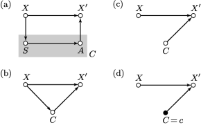
Figure 1: Directed acyclic graphs representing a basic control process. (a) Full control system with a sensor $S$ and an actuator $A$. (b) Reduced closed-loop diagram obtained by merging the sensor and the actuator into a single controller device, the controller. (c) Reduced open-loop control diagram. (d) Single actuation channel enacted by the controller’s state $C=c$.

In this section, we introduce a simple control model that allows investigation of the dynamical interplay that exists between a sensor and an actuator to ‘move’ a system from an unknown initial state to a desired final target state. Such a process is depicted schematically in Figure 1 in the form of directed acyclic graphs, also known as Bayesian networks pearl1988 ; jordan1999 . The vertices of these graphs correspond to random variables representing the state of a (classical) system; the arrows give the probabilistic dependencies among the random variables according to the general decomposition

$$p(x_{1},x_{2},\ldots,x_{N})=\prod_{i=1}^{N}p(x_{i}|\pi[X_{i}]),$$ (1)

where $\pi[X_{i}]$ is the set of random variables which are direct parents of $X_{i}$, $i=1,2,\ldots,N$, ($\pi[X_{1}]=\emptyset$). The acyclic condition of the graphs ensures that no vertex is a descendant or an ancestor of itself, in which case we can order the vertices chronologically, i.e., from ancestors to descendants. This defines a causal ordering, and, consequently, a time line directed on the graphs from left to right.

In the control graph of Figure 1a, the random variable $X$ represents the initial state of the system to be controlled, and whose values $x\in\mathcal{X}$ are drawn according to a fixed probability distribution $p_{X}(x)$ . In conformity with our introductory description of controllers, this initial state is controlled to a final state $X^{\prime}$ with state values $x^{\prime}\in\mathcal{X}$ by means of a sensor, of state variable $S$, and an actuator whose state variable $A$ influences the transition from $X$ to $X^{\prime}$. For simplicity, all the random variables describing the different systems are taken to be discrete random variables with finite sets of outcomes. The extension to continuous-state systems is discussed in Section IV. Also, to further simplify the analysis of this model, we assume throughout this paper that the sensor and the actuator are merged into a single device, called the controller, which fulfills both the roles of estimation and actuation (see Figure 1b). The state of the controller is denoted by $C$, and assumes values from some set $\mathcal{C}$ of admissible controls note1 .

Using this notation together with the decomposition of Eq.(1), the joint distribution $p(x,x^{\prime},c)$ describing the causal dependencies between the states of the control graphs can now be constructed. For instance, the complete joint distribution corresponding to the closed-loop graph of Figure 1b is written as

$$p(x,x^{\prime},c)_{\text{closed}}=p_{X}(x)p(c|x)p(x^{\prime}|x,c),$$ (2)

while the open-loop version of this graph, depicted in Figure 1c, is characterized by a joint distribution of the form

$$p(x,x^{\prime},c)_{\text{open}}=p_{X}(x)p_{C}(c)p(x^{\prime}|x,c).$$ (3)

Following the definition of closed- and open-loop control given above, what distinguishes probabilistically and graphically both control strategies is the presence, for closed-loop control, of a direct correlation link between $X$ and $C$ represented by the conditional probability $p(c|x)$. This correlation can be thought of as a (possibly noisy) communication channel, referred here to as the sensor or measurement channel, that enables the controller to gather an amount of information identified formally with the mutual information

$$I(X;C)=\sum_{x\in\mathcal{X},c\in\mathcal{C}}p_{XC}(x,c)\log\frac{p_{XC}(x,c)}{p_{X}(x)p_{C}(c)},$$ (4)

where $p_{X,C}(x,c)=p_{X}(x)p(c|x)$. (All logarithms are assumed to the base 2, except where explicitly noted.) Recall that $I(X;C)\geq 0$ with equality if and only if the random variables $X$ and $C$ are statistically independent cover1991 , so that in view of this quantity we are naturally led to define open-loop control with the requirement that $I(X;C)=0$; closed-loop control, on the other hand, must be such that $I(X;C)\neq 0$.

As for the actuation part of the control process, the joint distributions of Eqs.(2)-(3) show that it is accounted for by the channel-like probability transition matrix $p(x^{\prime}|x,c)$. The entries of this actuation matrix give the probability that the controlled system in state $X=x$ is actuated to $X^{\prime}=x^{\prime}$ given that the controller’s state is $C=c$. From here on, it will be convenient to think of the control actions indexed by each value of $C$ as a set of  actuation channels, with memoryless transition matrices

$$p(x^{\prime}|x)_{c}=p(x^{\prime}|x,c),$$ (5)

governing the transmission of the random variable $X$ to a target state $X^{\prime}$. In terms of the control graphs, such channels are represented in the same form as in Figure 1d to show that the fixed value $C=c$ (filled circle in the graph) enacts a transformation of the random variable $X$ (open circle) to a yet unspecified value associated with the random variable $X^{\prime}$ (open circle as well). Guided by this graphical representation, we will show in the next section that the overall action of a controller can be decomposed into a series of single conditional actuation actions or subdynamics triggered by the internal state of $C$.

Here we characterize the effect of the subdynamics available to a controller on the entropy of the initial state $X$:

$$H(X)=-\sum_{x\in\mathcal{X}}p_{X}(x)\log p_{X}(x).$$ (6)

In theory, this effect is completely determined by the choice of the initial state $X$, and the form of the actuation matrices. The effect of these two ‘variables’ on $H(X)$ is categorized according to the three following classes of dynamics:

One-to-one transitions: A given control subdynamics specified by $C=c$ conserves the entropy of the initial state $X$ if the corresponding probability matrix $p(x^{\prime}|x)_{c}$ is that of a noiseless channel. Permutations or translations of $X$ are examples of this sort of dynamics.

Many-to-one transitions: A control channel $p(x^{\prime}|x)_{c}$ may cause some subset $\mathcal{X}_{c}$ of the state space $\mathcal{X}$ to be mapped onto a smaller subset of values for $X^{\prime}$. In this case, the corresponding subdynamics is said to be dissipative or  volume-contracting as it decreases the entropy of ensembles of states lying in $\mathcal{X}_{c}$.

One-to-many transitions: A channel $p(x^{\prime}|x)_{c}$ can also lead $H(X)$ to increase if it is non-deterministic, i.e., if it specifies the image of one or more values of $X$ only up to a certain probability different than zero or one. This will be the case, for example, if the actuator is unable to accurately manipulate the dynamics of the controlled system, or if any part of the control system is affected by external and non-controllable systems.

From a strict mathematical point of view, note that any non-deterministic channel modeling a source of noise at the level of actuation or estimation can be represented abstractly as a randomly selected deterministic channel with transition matrix containing only zeros and ones. The outcome of a random variable undisclosed to the controller can be thought of as being responsible for the choice of the channel to use. Figure 2 shows specifically how this can be done by supplementing our original control graphs of Figure 1 with an exogenous and non-controllable random variable $Z$ in order to ‘purify’ the channel considered (actuation or estimation) note2 . For the actuation channel, as for instance, the purification condition simply refers to the two following properties:

(i) The mapping from $X$ to $X^{\prime}$ conditioned on the values $c$ and $z$, as described by the extended transition matrix $p(x^{\prime}|x,c,z)$, is deterministic for all $c\in\mathcal{C}$ and $z\in\mathcal{Z}$;

(ii) When traced out of $Z$, $p(x^{\prime}|x,c,z)$ reproduces the dynamics of $p(x^{\prime}|x,c)$, i.e.,

$$p(x^{\prime}|x,c)=\sum_{z\in\mathcal{Z}}p(x^{\prime}|x,c,z)p_{Z}(z),$$ (7)

for all $x^{\prime}$, $x\in\mathcal{X}$, and all $c\in\mathcal{C}$.

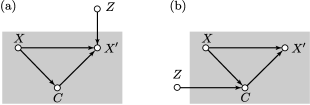
Figure 2: Control diagrams illustrating the purification procedure for (a) the actuation channel, and (b) the sensor channel. Purifying a channel, for instance the sensor channel, simply means that knowing the value of $X$ and $Z$ enables one to know with probability one the value of $C$. However, discarding (viz, tracing out) any information concerning $Z$ leaves us with some uncertainty as to which $C$ is reached from a given value for $X$.

III Conditional analysis

To complement the material introduced in the previous section, we now present a technique for analyzing the control graphs that emphasizes further the conceptual importance of the actuation channel and its graphical representation. The technique is based on a useful symmetry of Figure 1c that enables us to separate the effect of the random variable $X$ in the actuation matrix from the effect of the control variable $C$. From one perspective, the open-loop decomposition

$$p_{X^{\prime}}(x^{\prime})_{\text{open}}=\sum_{c}p_{C}(c)\left[\sum_{x}p(x^{\prime}|x,c)p_{X}(x)\right]$$ (8)

suggests that an open-loop control process can be decomposed into an ensemble of actuations, each one indexed by a particular value $c$ that takes the initial distribution $p_{X}(x)$ to a conditional distribution (first sum in parentheses)

$$p(x^{\prime}|c)_{\text{open}}=\sum_{x\in\mathcal{X}}p(x^{\prime}|x,c)p_{X}(x).$$ (9)

The final marginal distribution $p_{X^{\prime}}(x^{\prime})_{\text{open}}$ is then obtained by evaluating the second sum in Eq.(8), thus averaging $p(x^{\prime}|c)_{\text{open}}$ over the control variable. From another perspective, Eq.(8), re-ordered as

$$p_{X^{\prime}}(x^{\prime})_{\text{open}}=\sum_{x}p_{X}(x)\left[\sum_{c}p(x^{\prime}|x,c)p_{C}(c)\right],$$ (10)

indicates that the overall action of a controller can be seen as transmitting $X$ through an ‘averaged’ channel (sum in parentheses) whose transition matrix is given by

$$p(x^{\prime}|x)=\sum_{c\in\mathcal{C}}p(x^{\prime}|x,c)p_{C}(c).$$ (11)

In the former perspective, each actuation subdynamics represented by the control graph of Figure 1d can be characterized by a conditional open-loop entropy reduction defined by

$$\Delta H_{\text{open}}^{c}=H(X)-H(X^{\prime}|c)_{\text{open}}$$ (12)

where

$$H(X^{\prime}|c)=-\sum_{x^{\prime}\in\mathcal{X}}p(x^{\prime}|c)\log p(x^{\prime}|c).$$ (13)

(Subscripts of $H$ indicate from which distribution the entropy is to be calculated.) In the latter perspective, the entropy reduction associated with the unconditional transition from $X$ to $X^{\prime}$ is simply the open-loop entropy reduction

$$\Delta H_{\text{open}}=H(X)-H(X^{\prime})_{\text{open}}$$ (14)

which characterizes the control process as a whole, without regard to any knowledge of the controller’s state.

For closed-loop control, the decomposition of the control action into a set of conditional actuations seems a priori inapplicable, for the controller’s state itself depends on the initial state of the controlled system, and thus cannot be fixed at will. Despite this fact, one can use the Bayesian rule of statistical inference

$$p(x|c)=\frac{p(c|x)p_{X}(x)}{p_{C}(c)},$$ (15)

where

$$p_{C}(c)=\sum_{x\in\mathcal{X}}p(c|x)p_{X}(x),$$ (16)

to invert the dependency between $X$ and $C$ in the sensor channel so as to rewrite the closed-loop decomposition in the following form:

$$p_{X^{\prime}}(x^{\prime})_{\text{closed}}=\sum_{c}p_{C}(c)\left[\sum_{x}p(x^{\prime}|x,c)p(x|c)\right].$$ (17)

By comparing this last equation with Eq.(8), we see that a closed-loop controller is essentially an open-loop controller acting on the basis of $p(x|c)$ instead of $p_{X}(x)$ ho1964 . Thus, given that $c$ is fixed, a closed-loop equivalent of Eq.(12) can be calculated simply by substituting $p_{X}(x)$ with $p(x|c)$, thereby obtaining

$$\Delta H_{\text{closed}}^{c}=H(X|c)-H(X^{\prime}|c)$$ (18)

for all $c$.

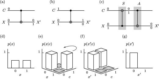
Figure 3: Controlled-not controller. (a) Boolean circuit illustrating the effect of the controller’s state $C=0$ on the input states ${0,1}$ of the controlled system $X$ (identity in this case). (b) Control action triggered by $C=1$ (swapping). (c) Complete control system with sensor $S$ and actuator $A$. Note that the sensor itself is modeled by a cnot gate. (d)-(g) State of the controlled system at different stages of the control depicted in the spirit of conditional analysis. (d) A uniformly distributed input state $X$ is measured by the sensor in such a way that the conditional random variable $X|c$ is deterministic (e). (f) The control action triggered by $C$ has the effect of swapping the values $x$ for which $C=1$. (g) Deterministic probability distribution for the final state $X^{\prime}$ upon averaging over $C$.

The rationale for decomposing a closed-loop control action into a set of conditional actuations can be justified by observing that a closed-loop controller, after the estimation step, can be thought of as an ensemble of open-loop controllers acting on a set of estimated states. In other words, what differentiates open-loop and closed-loop control from the viewpoint of the actuator is the fact that, for the former strategy, a given control action selected by $C=c$ transforms all the values $x$ contained in the support of $X$, i.e., the set

$$\text{supp}(X)=\{x\in\mathcal{X}:p_{X}(x)>0\},$$ (19)

whereas for the latter strategy, namely closed-loop control, the same actuation only affects the support of the posterior distribution $p(x|c)$ associated with $X|c$, the random variable $X$ conditioned on the outcome $c$ . This is so because the decision as to which control value is used has been determined according to the observation of specific values of $X$ which are in turn affected by the chosen control value. By combining the influence of all the control values, we thus have that information gathered by the sensor affects the entire control process by inducing a covering of the support space

$$\text{supp}(X)=\bigcup_{c\in\mathcal{C}}\text{supp}(X|c),$$ (20)

in such a way that values $x\in\text{supp}(X|c_{1})$, for a fixed $c_{1}\in\mathcal{C}$, are controlled by the corresponding actuation channel $p(x^{\prime}|x,C=c_{1})$, while other values in $\text{supp}(X|c_{2})$ are controlled using $p(x^{\prime}|x,C=c_{2})$, and so on for all $c_{i}\in\mathcal{C}$. This is manifest if one compares Eqs.(8) and (17). Note that a particular value $x$ included in $\text{supp}(X)$ may be actuated by many different control values if it is part of more than one ‘conditional’ support $\text{supp}(X|c)$. Hence the fact that Eq.(20 ) only specifies a covering, and not necessarily a partition constructed from non-overlapping sets. Whenever this occurs, we say that the control is mixing.

To illustrate the above ideas about subdynamics applied to conditional subsets of $\mathcal{X}$ in a more concrete setting, we proceed in the next paragraph with a basic example involving the control of a binary state system using a controller restricted to use permutations as actuation rules hugo12000 . This example will be used throughout the article as a test situation for other concepts.

Example 1. Let $C$ be a binary state controller acting on a bit $X$ by means of a so-called controlled-not (cnot) logical gate. As shown in the circuits of Figures 3a-b, the state $X$, under the action of the gate, is left intact or is negated depending on the control value:

$$x^{\prime}=\left\{\begin{array}[]{ll}x,&\text{if }c=0\\ x\oplus 1,&\text{if }c=1.\end{array}\right.$$ (21)

($\oplus$ stands for modulo $2$ addition.) Furthermore, assume that the controller’s state is determined by the outcome of a ‘perfect’ sensor which can be modeled by another cnot gate such that $C=X$ when $C$ is initially set to $0$ (Figure 3c). As a result of these actuation rules, it can be verified that $\Delta H_{\text{open}}^{c}=\Delta H_{\text{closed}}^{c}=0$ , and so the application of a single open- or closed-loop control action cannot increase the uncertainty $H(X)$. In fact, whether the subdynamics is applied in an open- or closed-loop fashion is irrelevant here: a permutation is just a permutation in either cases. Now, since $C=X$, we have that the random variable $X$ conditioned on $C=c$ must be equal to $c$ with probability one. For closed-loop control, this implies that the value $X=0$, which is the only element of $\text{supp}(X|C=0)$, is kept constant during actuation, whereas the value $X=1$ in $\text{supp}(X|C=1)$ is negated to $0$ in accordance with the controller’s state $C=1$ (Figure 3e). Under this control action, the conditional random variable $X^{\prime}|c$ is forced to assume the same deterministic value for all $c$, implying that $X^{\prime}$ must be deterministic as well, regardless of the statistics of $C$ (Figures 3f-g). Therefore, $H(X^{\prime})_{\text{closed}}=0$. In contrast, the application of the same actuation rules in an open-loop fashion transform the state $X$ to a final state having, at best, no less uncertainty than what is initially specified by the statistics of $X$, i.e., $H(X^{\prime})_{\text{open}}\geq H(X)$. $\blacksquare$

IV Entropic formulation of controllability and observability

The first instance of the general control problem that we now proceed to study involves the dual concepts of controllability and observability. In control theory, the importance of these concepts arises from the fact that they characterize mathematically the input-output structure of a system intended to be controlled, and thereby determine whether a given control task is realizable or not dazzo1988 ; singh1987 . In short, controllability is concerned with the possibilities and limitations of the actuation channel or, in other words, the class of control dynamics that can be effected by a controller. Observability, on the other hand, is concerned with the set of states which are accessible to estimation given that a particular sensor channel is used. In this section, prompted by preliminary results obtained by Lloyd and Slotine lloyd1996 , we define entropic analogs of the widely held control-theoretic definitions of controllability and observability, and explore the consequences of these new definitions.

IV.1 Controllability

In its simplest expression, a system is said to be controllable at $X=x$ if any of the final state $X^{\prime}=x^{\prime}$ can be reached from $X=x$ using at least one control input $C=c$ dazzo1988 ; singh1987 . Allowing for non-deterministic control actions, we may refine this definition and say that a system is perfectly controllable at $X=x$ if it is controllable at $X=x$ with probability 1, i.e., if, for any $x^{\prime}$, there exists at least one $c$ such that $p(x^{\prime}|x,c)=1$ . In other words, a system is perfectly controllable if (i) all final states for $X^{\prime}$ are reachable from $X=x$ (complete reachability condition); and (ii) all final states for $X^{\prime}$ are connected to $X=x$ by at least one deterministic subdynamics (deterministic transitions condition). In terms of entropy, these two conditions are translated as follows. (The next result was originally put forward in lloyd1996 without a complete proof.)

Theorem 1. A system is perfectly controllable at $X=x$ if and only if there exists a distribution $p(c|x)$ note3 such that

$$p(x^{\prime}|x)=\sum_{c\in\mathcal{C}}p(x^{\prime}|x,c)p(c|x)\neq 0$$ (22)

for all $x^{\prime}$, and

$$H(X^{\prime}|x,C)=\sum_{c\in\mathcal{C}}H(X^{\prime}|x,c)p(c|x)=0,$$ (23)

where

$$H(X^{\prime}|x,c)=-\sum_{x^{\prime}\in\mathcal{X}}p(x^{\prime}|x,c)\log p(x^{\prime}|x,c).$$ (24)

Proof. If $x$ is controllable, then for each $x^{\prime}$ there exists at least one control value $c=c(x^{\prime},x)\in\mathcal{C}$ such that $p(x^{\prime}|x,c)=1$, and thus $H(X^{\prime}|x,c)=0$. Also, choosing

$$\text{supp}(C|x)=\{c:p(x^{\prime}|x,c)=1\}$$ (25)

over all $x^{\prime}\in\mathcal{X}$ and $X=x$ ensures that the average conditional entropy over the conditional random variable $C|x$ vanishes, and that $p(x^{\prime}|x)\neq 0$. This proves the direct part of the theorem. To prove the converse, note that if $p(x^{\prime}|x)\neq 0$ for a given $x^{\prime}$, then there is at least one value $c$ for which $p(x^{\prime}|x,c)\neq 0$, which means that there is at least one subdynamics connecting $x$ to $x^{\prime}$. If in addition we have $H(X^{\prime}|x,C)=0$, then we can conclude that such a subdynamics must in fact be deterministic. As this is verified for any state value $x^{\prime}$, we obtain in conclusion that for all $x^{\prime}\in\mathcal{X}$ there exists a $c$ such that $p(x^{\prime}|x,c)=1$. $\blacksquare$

In the case where a system is only approximately controllable, i.e., controllable but not in a deterministic fashion, the conditional entropy $H(X^{\prime}|x,C)$ has the desirable feature of being interpretable as the residual uncertainty or uncontrolled variation left in the output $X^{\prime}$ when the controller’s state $C$ is chosen with respect to the initial value $x$ lloyd1996 . If one regards $C$ as an input to a communication channel and $X^{\prime}$ as the channel output, then the degree to which the final state $X^{\prime}$ is controlled by manipulating the controller’s state can be identified with the conditional mutual information $I(X^{\prime};C|x)$. This latter quantity can be expressed either using a formula similar to Eq.(4), or by using the expression

$$I(X^{\prime};C|x)=H(X^{\prime}|x)-H(X^{\prime}|x,C),$$ (26)

which is a conditional version of the chain rule

$$I(X;Y)=H(X)-H(X|Y),$$ (27)

valid for any random variables $X$ and $Y$.

Note that the two above equations allow for another interpretation of $H(X^{\prime}|x,C)$. The conditional entropy $H(X|Y)$, entering in (27 ), is often interpreted in communication theory as representing an information loss (the so-called equivocation of Shannon shannon1948 ), which results from substracting the maximum noiseless capacity $I(X;X)=H(X)$ of a communication channel with input $X$ and output $Y$ from the actual capacity of that channel as measured by $I(X;Y)$. In our case, we can apply the same reasoning to Eq.(26), and interpret the quantity $H(X^{\prime}|x,C)$ as a control loss which appears as a negative contribution in the expression of $I(X^{\prime};C|x)$, the number of bits of accuracy to which specifying the control variable specifies the output state of the controlled system. This means that higher is the quantity $H(X^{\prime}|x,C)$, then higher is the uncertainty or imprecision associated with the outcome of $X^{\prime}$ upon application of the control action.

IV.2 Complete and average controllability

In order to characterize the complete controllability of a system, i.e., its controllability properties over all possible initial states, define

$$L_{C} = \min_{\{p(c|x)\}}H(X^{\prime}|X,C)$$ (28)

$$= \min_{\{p(c|x)\}}\sum_{x\in\mathcal{X}}p_{X}(x)\sum_{c\in\mathcal{C}}H(X^{\prime}|x,c)p(c|x)$$

as the average control loss. (The minimization over all conditional distributions for $C$ is there to ensure that $L_{C}$ reflects the properties of the actuation channel, and does not depend on one’s choice of control inputs.) With this definition, we have that a system is perfectly controllable over the support of $X$ if $L_{C}=0$ and $p(x^{\prime}|x)\neq 0$ for all $x^{\prime}$. In any other cases, it is approximately controllable for at least one $x$. The proof of this result follows essentially by noting that, since discrete entropy is positive definite, the condition $H(X^{\prime}|X,C)=0$ necessarily implies $H(X^{\prime}|x,C)=0$ for all $x\in\text{supp}(X)$.

The next two results relate the average control loss with other quantities of interest. Control graphs containing the purification of the actuation channel, as depicted in Figure 2, are used throughout the rest of this section.

Theorem 2. Under the assumption that $X^{\prime}$ is a deterministic random variable conditioned on the values $x$, $c$, and $z$ (purification assumption), we have $L_{C}\leq H(Z)$ with equality if, and only if, $H(Z|X^{\prime},X,C)=0$.

Proof. Using the general inequality $H(X)\leq H(X,Y)$, and the chain rule for joint entropies, one may write

$$H(X^{\prime}|X,C) \leq H(X^{\prime},Z|X,C)$$ (29)

$$= H(Z|X,C)+H(X^{\prime}|X,C,Z).$$

However, $H(X^{\prime}|X,C,Z)=0$, since the knowledge of the triplet $(x,c,z)$ is sufficient to infer the value of $X^{\prime}$ (see the conditions in Section II). Hence,

$$H(X^{\prime}|X,C) \leq H(Z|X,C)$$ (30)

$$= H(Z),$$

where the last equality follows from the fact that $Z$ is chosen independently of $X$ and $C$ as illustrated in the control graph of Figure 2a. Now, from the chain rule

$$H(X^{\prime},Z|X,C)=H(X^{\prime}|X,C)+H(Z|X^{\prime},X,C),$$ (31)

it is clear that equality in the first line of expression (29) is achieved if and only if $H(Z|X^{\prime},X,C)=0$. $\blacksquare$

The result of Theorem 2 demonstrates that the uncertainty associated with the control of the state $X$ is upper bounded by the noise level of the actuation channel as measured by the entropy of $Z$. This agrees well with the fact that one goal of controllers is to protect a system against the effects of its environment so as to ensure that it is minimally affected by noise. In the limit where the control loss vanishes, the state $X^{\prime}$ of the controlled system should show no variability given that we know the initial state and the control action, even in the presence of actuation noise, and should thus be independent of the random variable $Z$. This is the essence of the next two results which hold for the same conditions as Theorem 2 (the minimization over the set of conditional probability distributions $\{p(c|x)\}$ is implied at this point).

Theorem 3. $L_{C}=I(X^{\prime};Z|X,C)$.

Proof. From the chain rule of mutual information, we can easily derive

$$I(X^{\prime};Z|X,C)=H(X^{\prime}|X,C)-H(X^{\prime}|X,C,Z).$$ (32)

Thus, $I(X^{\prime};Z|X,C)=H(X^{\prime}|X,C)$ if we use again the deterministic property of the random variable $X^{\prime}|x,c,z$ upon purification of $p(x^{\prime}|x,c)$. $\blacksquare$

Theorem 4. $L_{C}=I(X^{\prime};X,C,Z)-I(X^{\prime};X,C)$.

Proof. Using the chain rule of mutual information, we write

$$I(X^{\prime};X,C,Z) = H(X^{\prime})-H(X^{\prime}|X,C,Z)$$ (33)

$$= H(X^{\prime})-H(X^{\prime}|X,C,Z)$$

$$+H(X^{\prime}|X,C)-H(X^{\prime}|X,C)$$

$$= I(X^{\prime};X,C)+I(X^{\prime};Z|X,C).$$

For the last equality, we have used Eq.(32). Now, by substituting $L_{C}=I(X^{\prime};Z|X,C)$ from the previous theorem, we obtain the desired result. $\blacksquare$

As a direct corollary of these two results, we have that a system is completely and perfectly controllable if, and only if, $I(X^{\prime};Z|X,C)$ is equal to zero or equivalently if, and only if,

$$I(X^{\prime};X,C,Z)=I(X^{\prime};X,C).$$ (34)

Hence, a necessary and sufficient entropic condition for perfect controllability is that the final state of the controlled system, after the actuation step, is statistically independent of the noise variable $Z$ given $X$ and $C$. In that case, the ‘information’ $I(X^{\prime};Z|X,C)$ conveyed in the form of noise from $Z$ to the controlled system is zero. Another ‘common sense’ interpretation of this result can be given if the quantity $I(X^{\prime};Z|X,C)$ is instead viewed as representing the ‘information’ about $X^{\prime}$ that has been transferred to the non-controllable state $Z$ in the form of ‘lost’ correlations.

This analysis of control systems in terms of noise and information protection is similar to that of error-correcting codes. The design of error-correcting codes is closely related to that of control systems: the information duplicated by a code, when corrupted by noise, is used to detect errors (sensor step) which are then corrected by enacting specific correcting or erasure actions (actuation step) shannon1948 ; roman1992 ; cerf1997 . The analogy to error-correcting codes can be strengthened even further if probabilities accounting for undetected and uncorrected errors are modeled by means of communication channels similar to the sensor and actuation channels. In this context, whether or not a prescribed set of erasure actions is sufficient to correct for a particular type of errors is determined by the control loss.

IV.3 Observability

The concept of observability is concerned with the issue of inferring the state $X$ of the controlled system based on some knowledge or data of the state provided by a measurement apparatus, taken here to correspond to $C$. More precisely, a controlled system is termed perfectly observable if the sensor’s transition matrix $p(c|x)$ maps no two values of $X$ to a single observational output value $c$, or in other words if for all $c\in\mathcal{C}$ there exists only one value $x$ such that $p(x|c)=1$. As a consequence, we have the following result lloyd1996 . (We omit the proof which readily follows from well-known properties of entropy.)

Theorem 5. A system with state variable $X$ is perfectly observable, with respect to all observed value $c\in\text{supp}(C)$, if and only if

$$H(X|C)=\sum_{c\in\mathcal{C}}H(X|c)p_{C}(c)=0.$$ (35)

The information-theoretic analog of a perfectly observable system is a lossless communication channel $X\rightarrow Y$ characterized by $H(X|Y)=0$ for all input distributions cover1991 . As a consequence of this association, we interpret the conditional entropy $H(X|C)$ as the information loss, or sensor loss, of the sensor channel, denoted by $L_{S}$. We now extend our results on controllability into the domain of observability. The first question that arises is, given the similarity between the average control loss $L_{C}$ and the sensor loss, do we obtain true results for observability by merely substituting $L_{C}$ by $L_{S}$ in Theorems 2 and 3?

The answer is no: the fact that a communication channel is lossless has nothing to do with the fact that it can be non-deterministic. An example of such a channel is one that maps the singleton input set $\mathcal{X}=\{0\}$ to multiple instances of the output set $\mathcal{C}$ with equal probabilities. This is clearly a non-deterministic channel, and yet since there is only one possible value for $X$, the conditional entropy $H(X|c)$ must be equal to zero for all $c\in\mathcal{C}$. Hence, contrary to Theorem 2, the observation loss $L_{S}$ cannot be bounded above by the entropy of the random variable responsible for the non-deterministic properties of the sensor channel. However, we are not far from a similar result: by analyzing the meaning of the sensor loss a bit further, the generalization of Theorem 2 for observability can in fact be derived using the ‘backward’ version of the sensor channel. More precisely, $L_{S}\leq H(Z_{B})$ where $Z_{B}$ is now the random variable associated with the purification of the transition matrix $p(x|c)$. To prove this result, the reader may revise the proof of Theorem 2, and replace the forward purification condition $H(C|X,Z)=0$ for the sensor channel by its backward analog $H(X|C,Z_{B})=0$.

To close this section, we present next what is left to generalization of the results on controllability. One example aimed at illustrating the interplay between the controllability and observability properties of a system is also given.

Theorem 6. If the state $X$ is perfectly observable, then $I(X;Z|C)=0$. (The random variable $Z$ stands for the purification variable of the ‘forward’ sensor channel $p(c|x)$.)

Proof. The proof is rather straightforward. Since $H(X|C)\geq H(X|C,Z)$, the condition $L_{S}=0$ implies $H(X|C,Z)=0$. Thus by the chain rule

$$I(X;Z|C)=H(X|C)-H(X|C,Z),$$ (36)

we conclude with $I(X;Z|C)=0$. $\blacksquare$

Corollary 7. If $L_{S}=0$, then $I(X;C,Z)=I(X;C)$.

The interpretations of the two above results follow closely those given for controllability. We will not discuss these results further except to mention that, contrary to the case of controllability, $I(X;Z|C)=0$ is not a sufficient condition for a system to be observable. This follows simply from the fact that $I(X;Z|C)=0$ implies $H(X|C)=H(X|C,Z)$, and at this point the purification condition $H(C|X,Z)=0$ for the sensor channel is of no help to obtain $H(X|C)=0$.

Example 2. Consider again the control system of Figure 3. Given the actuation rules described by the cnot logical gate, it can be verified easily that for $X=0$ or $1$, $H(X^{\prime}|x,C)=0$ and $p(x^{\prime}|x)\neq 0$ for all $x^{\prime}$. Therefore, the controlled system is completely and perfectly controllable. This implies, in particular, that $\Delta H_{\text{open}}^{c}=\Delta H_{\text{closed}}^{c}=0$, and that the final state of the controlled system may be actuated to a single value with probability 1, as noted before. For the latter observation, note that $X^{\prime}=x^{\prime}$ with probability 1 so long as the initial state $X$ is known with probability 1 (perfectly observable). In general, if a system is perfectly controllable (actuation property) and perfectly observable (sensor property), then it is possible to perfectly control its state to any desired value with vanishing probability of error. In such a case, we can say that the system is closed-loop controllable. $\blacksquare$

IV.4 The case of continuous random variables

The concept of a deterministic continuous random variable is somewhat ill-defined, and, in any case, cannot be associated with the condition $H(X)=0$ formally. (Consider, e.g., the peaked distribution $p(x)=\delta(x-x_{0})$ which is such that $H(X)=-\infty$.) To circumvent this difficulty, controllability and observability for continuous random variables may be extended via a quantization or coarse-graining of the relevant state spaces cover1991 . For example, a continuous-state system can be defined to be perfectly controllable at $x$ if for every final destination $x^{\prime}$ there exists at least one control value $c$ which forces the system to reach a small neighborhood of radius $\Delta>0$ around $x^{\prime}$ with probability 1. Equivalently, $x$ can be termed perfectly controllable to accuracy $\Delta$ if the variable $x^{\Delta}$ obtained by quantizing $\mathcal{X}$ at a scale $\Delta$ is perfectly controllable. Similar definitions involving quantized random variables can also be given for observability. The recourse to the quantized description of continuous variables has the virtue that $H(X^{\Delta})$ and $H(X^{\Delta}|C^{\Delta})$ are well-defined functions which cannot be infinite. It is also the natural representation used for representing continuous-state models on computers.

V Stability and entropy reduction

The emphasis in the previous section was on proving upper limits for the control and the observation loss, and on finding conditions for which these losses vanish. In this section, we depart from these quantities to focus our attention on other measures which are interesting in view of the stability properties of a controlled system. How can a system be stabilized to a target state or a target subset (attractor) of states? Also, how much information does a controller need to gather in order to achieve successfully a stabilization procedure? To answer these questions, we first propose an entropic criterion of stability, and justify its usefulness for problems of control. In a second step, we investigate the quantitative relationship between the closed-loop mutual information $I(X;C)$ and the gain in stability which results from using information in a control process.

V.1 Stochastic stability

Intuitively, a stable system is a system which, when activated in the proximity of a desired operating point, stays relatively close to that point indefinitely in time, even in the presence of small perturbations. In the field of control engineering, there exist several formalizations of this intuition, some less stringent than others, whose range of applications depend on theoretical as well as practical considerations. It would be impossible, and, perhaps inappropriate, to review here all the definitions of stability currently used in the study and design of control systems; for our purposes, it suffices to say that a necessary condition for stabilizing a dynamical system is to be able to decrease its entropy, or immunize it from sources of entropy like those associated with environment noise, motion instabilities, and incomplete specification of control conditions. This entropic aspect of stabilization is implicit in almost all criteria of stability insofar as a probabilistic description of systems focusing on sets of responses, rather than on individual response one at a time, is adopted stengel1994 ; schlo1980 ; shaw1981 ; farmer1982 . In this sense, what is usually sought in controlling a system is to confine its possible states, trajectories or responses within a set as small as possible (low entropy final state) starting from a wide range of initial states or initial conditions (high entropy initial random state).

The fundamental role of entropy reduction in control suggests the two following problems. First, given the initial state $X$ and its entropy $H(X)$ , a set of actuation subdynamics, and the type of controller (open- or closed-loop), what is the maximum entropy reduction achievable during the controlled transition from $X$ to $X^{\prime}$? Second, what is the quantitative relationship between the maximal open-loop entropy reduction and the closed-loop entropy reduction? Note that for control purposes it does not suffice to reduce the entropy of $X^{\prime}$ conditionally on the state of another system (the controller in particular). For instance, the fact that $H(X^{\prime}|C)$ vanishes for a given controller acting on a system does not imply by itself that $H(X^{\prime})$ must vanish as well, or that $X^{\prime}$ is stabilized. What is required for control is that actuators modify the dynamics of the system intended to be controlled by acting directly on it, so as to reduce the marginal entropy $H(X^{\prime})$ . This unconditional aspect of stability has been discussed in more detail in hugo12000 ; hugo22000 .

V.2 Open-loop control optimality

Using the concavity property of entropy, and the fact that $\Delta H_{\text{ open}}$ is upper bounded by the maximum of $\Delta H_{\text{open}}^{c}$ over all control values $c$, we show in this section that the maximum decrease of entropy achieved by a particular subdynamics of control variable

$$\hat{c}=\arg\max_{c\in\mathcal{C}}\Delta H_{\text{open}}^{c}$$ (37)

is open-loop optimal in the sense that no random (i.e., non-deterministic) choice of the controller’s state can improve upon that decrease. More precisely, we have the following results. (Theorem 9 was originally stated without a proof in hugo12000 .)

Lemma 8. For any initial state $X$, the open-loop entropy reduction $\Delta H_{\text{open}}$ satisfies

$$\Delta H_{\text{open}}\leq\Delta H_{\text{open}}^{C},$$ (38)

where

$$\Delta H_{\text{open}}^{C} = \sum_{c\in\mathcal{C}}p_{C}(c)\Delta H_{\text{ open }}^{c}$$ (39)

$$= H(X)-H(X^{\prime}|C)_{\text{open}}$$

with $\Delta H_{\text{open}}^{c}$ defined as in Eq.(12). The equality is achieved if and only if $I(X^{\prime};C)=0$.

Proof. Using the inequality $H(X^{\prime})\geq H(X^{\prime}|C)$, we write directly

$$\Delta H_{\text{open}} = H(X)-H(X^{\prime})_{\text{open}}$$ (40)

$$\leq H(X)-H(X^{\prime}|C)_{\text{open}}.$$

Now, let us prove the equality part. If $C$ is statistically independent of $X^{\prime}$, then $H(X^{\prime}|C)=H(X^{\prime})$, and

$$\Delta H_{\text{open}}=\Delta H_{\text{open}}^{C}.$$ (41)

Conversely, the above equality implies $H(X^{\prime}|C)=H(X^{\prime})$, and thus we must have that $C$ is independent of $X^{\prime}$. $\blacksquare$

Theorem 9. The entropy reduction achieved by a set of actuation subdynamics used in open-loop control is always such that

$$\Delta H_{\text{open}}\leq\max_{c\in\mathcal{C}}\Delta H_{\text{open}}^{c},$$ (42)

for all $p_{X}(x)$. The equality can always be achieved for the deterministic controller $C=\hat{c}$, with $\hat{c}$ defined as in Eq.(37).

Proof. The average conditional entropy $H(X^{\prime}|C)$ is always such that

$$\min_{c\in\mathcal{C}}H(X^{\prime}|c)\leq\sum_{c\in\mathcal{C}}p_{C}(c)H(X^{\prime}|c).$$ (43)

Therefore, making use of the previous lemma, we obtain

$$\Delta H_{\text{open}} \leq \Delta H_{\text{open}}^{C}$$ (44)

$$\leq H(X)-\min_{c\in\mathcal{C}}H(X^{\prime}|c)$$

$$= \max_{c\in\mathcal{C}}\Delta H_{\text{open}}^{c}.$$

Also, note that if $C=\hat{c}$ with probability 1, then the two above inequalities are saturated since in this case $I(X^{\prime};C)=0$ and $\Delta H_{\text{open}}^{C}=\Delta H_{\text{open}}^{\hat{c}}$. $\blacksquare$

An open-loop controller or a control strategy is called pure if the control random variable $C$ is deterministic, i.e., if it assumes only one value with probability 1. An open-loop controller that is not pure is called mixed. (We also say that a mixed controller activates a mixture of control actions.) In view of these definitions, what we have just proved is that a pure controller with $C=\hat{c}$ is necessarily optimal; any mixture of the control variable either achieves the maximum entropy decrease prescribed by Eq.(42) or yields a smaller value. As shown in the next example, this is so even if the actuation subdynamics used in the control process are deterministic.

Example 3. For the cnot controller of Example 1, we noted that $H(X^{\prime})_{\text{open}}=H(X)$, or equivalently that $\Delta H_{\text{open}}=0$, only at best. To be more precise, $\Delta H_{\text{ open}}=0$ only if a pure controller is used or if $H(X)=1$ bit (already at maximum entropy). If the control is mixed, and if $H(X)<1$ bit, then $\Delta H_{\text{open}}$ must necessarily be negative. This is so because uncertainty as to which actuation rule is used must imply uncertainty as to which state the controlled system is actuated to. $\blacksquare$

Note that purity alone is not a sufficient condition for open-loop optimality, nor it is a necessary one in fact. To see this, note on the one hand that a pure controller having

$$C=\arg\min_{c\in\mathcal{C}}\Delta H_{\text{open}}^{c}$$ (45)

with probability one is surely not optimal, unless all entropy reductions $\Delta H_{\text{open}}^{c}$ have the same value. On the other hand, to prove that a mixed controller can be optimal, note that if any subset $\mathcal{C}_{o}\subseteq\mathcal{C}$ of actuation subdynamics is such that $p(x^{\prime}|c)=p_{X^{\prime}}(x^{\prime})$, and $\Delta H_{\text{open}}^{c}$ assumes a constant value for all $c\in\mathcal{C}_{o}$, then one can build an optimal controller by choosing a non-deterministic distribution $p(c)$ with $\text{ supp}(C)=\mathcal{C}_{o}$.

V.3 Closed-loop control optimality

The distinguishing characteristic of an open-loop controller is that it usually fails to operate efficiently when faced with uncertainty and noise. An open-loop controller acting independently of the state of the controlled system, or solely based on the statistical information provided by the distribution $p_{X}(x)$, cannot reliably determine which control subdynamics is to be applied in order for the initial (a priori unknown) state $X$ to be propagated to a given target state. Furthermore, an open-loop control system cannot compensate actively in time for any disturbances that add to the actuator’s driving state (actuation noise). To overcome these difficulties, the controller must be adaptive: it must be capable of estimating the unpredictable features of the controlled system during the control process, and must be able to use the information provided by estimation to decide of specific control actions, just as in closed-loop control.

A basic closed-loop controller was presented in Example 1. For this example, we noted that the perfect knowledge of the initial state’s value ($X=0$ or $1$) enabled the controller to decide which actuation subdynamics (identity or permutation) is to be used in order to actuate the system to $X^{\prime}=0$ with probability 1. The fact that the sensor gathers $I(X;C)=H(X)$ bits of information during estimation is a necessary condition for this specific controller to achieve $H(X^{\prime})_{\text{closed}}=0$, since having $I(X;C)<H(X)$ may result in generating the value $X^{\prime}=1$ with non-vanishing probability. In general, just as a subdynamics mapping the input states $\{0,1\}$ to the single value $\{0\}$ would require no information to force $X^{\prime}$ to assume the value $0$, we expect that the closed-loop entropy reduction should not only depend on $I(X;C)$, the effective information available to the controller, but should also depend on the reduction of entropy attainable by open-loop control. The next theorem, which constitutes the main result of this work, embodies exactly this statement by showing that one bit of information gathered by the controller has a maximum value of one bit in the improvement of entropy reduction that closed-loop gives over open-loop control.

Theorem 10. The amount of entropy

$$\Delta H_{\text{closed}}=H(X)-H(X^{\prime})_{\text{closed}}$$ (46)

that can be extracted from a system with given initial state $X$ by using a closed-loop controller with fixed set of actuation subdynamics satisfies

$$\Delta H_{\text{closed}}\leq\Delta H_{\text{open}}^{\max}+I(X;C).$$ (47)

where

$$\Delta H_{\text{open}}^{\max}=\max_{p_{X}(x)\in\mathcal{P},c\in\mathcal{C}}\Delta H_{\text{open}}^{c}$$ (48)

is the maximum entropy decrease that can be obtained by (pure) open-loop control over any input distribution chosen in the set $\mathcal{P}$ of all probability distributions.

A proof of the result, based on the conservation of entropy for closed systems, was given in hugo12000 following results found in lloyd1989 ; caves1996 . Here, we present an alternative proof based on conditional analysis which has the advantage over our previous work to give some indications about the conditions for equality in (47). Some of these conditions are derived in the next section.

Proof. Given that $\Delta H_{\text{open}}^{\max}$ is the optimal entropy reduction for open-loop control over any input distribution, we can write

$$H(X^{\prime})_{\text{open}}\geq H(X)-\Delta H_{\text{open}}^{\max}.$$ (49)

Now, using the fact that a closed-loop controller is formally equivalent to an ensemble of open-loop controllers acting on the conditional supports $\text{supp}(X|c)$ instead of $\text{supp}(X)$, we also have for all $c\in\mathcal{C}$

$$H(X^{\prime}|c)_{\text{closed}}\geq H(X|c)-\Delta H_{\text{open}}^{\max},$$ (50)

and, on average,

$$H(X^{\prime}|C)_{\text{closed}}\geq H(X|C)-\Delta H_{\text{open}}^{\max}.$$ (51)

That $\Delta H_{\text{open}}^{\max}$ must enter in the lower bounds of $H(X^{\prime})_{\text{open}}$ and $H(X^{\prime})_{\text{closed}}$ can be explained in other words by saying that each conditional distribution $p(x|c)$ is a legitimate input distribution for the initial state of the controlled system. It is, in any cases, an element of $\mathcal{P}$. This being said, notice now that $H(X^{\prime})\geq H(X^{\prime}|C)$ implies

$$H(X^{\prime})_{\text{closed}}\geq H(X|C)-\Delta H_{\text{open}}^{\max}.$$ (52)

Hence, we obtain

$$\Delta H_{\text{closed}} \leq H(X)-H(X|C)+\Delta H_{\text{closed}}^{\max}$$ (53)

$$= I(X;C)+\Delta H_{\text{closed}}^{\max},$$

which is the desired upper bound. To close the proof, note that $\Delta H_{\text{open}}^{\max}$ cannot be evaluated using the initial distribution $p_{X}(x)$ alone because the maximum reduction of entropy in open-loop control starting from $p_{X}(x)$ may differ from the reduction of entropy obtained when some actuation channel is applied in closed-loop to $p(x|c)$. See hugo22000 for a specific example of this. $\blacksquare$

The above theorem enables us to finally understand all the results of Example 1. As noted already, since the actuation subdynamics consist of permutations, we have $\Delta H_{\text{open}}^{\max}=0$ for any distribution $p_{X}(x)$. Thus, we should have $\Delta H_{\text{closed}}\leq I(X;C)$. For the particular case studied where $C=X$, the controller is found to be optimal, i.e., it achieves the maximum possible entropy reduction $\Delta H_{\text{closed}}=I(X;C)$. This proves, incidentally, that the bound of inequality (47) is tight. In general, we may define a control system to be optimal in terms of information if the gain in stability obtained by substracting $H(X^{\prime})_{\text{open}}$ from $H(X^{\prime})_{\text{closed}}$ is exactly equal to the sensor mutual information $I(X;C)$. Equivalently, a closed-loop control system is optimal if its efficiency $\eta$, defined by

$$\eta=\frac{H(X^{\prime})_{\text{open}}-H(X^{\prime})_{\text{closed}}}{I(X;C)},$$ (54)

is equal to 1.

Having determined that optimal controllers do exist, we now turn to the problem of finding general conditions under which a given controller is found to be either optimal ($\eta=1$) or sub-optimal ($\eta<1$). By analyzing thoroughly the proof of Theorem 10, one finds that the assessment of the condition $I(X^{\prime};C)=0$, which was not a sufficient condition for open-loop optimality, is again not sufficient here to conclude that a closed-loop controller is optimal. This comes as a result of the fact that not all control subdynamics applied in a closed-loop fashion are such that $\Delta H_{\text{closed}}^{c}=\Delta H_{\text{open}}^{\max}$ in general. Therefore the average final condition entropy $H(X^{\prime}|C)_{\text{ closed }}$ need not necessarily be equal to the bound imposed by inequality ( 51). However, in a scenario where the entropy reductions $\Delta H_{\text{ open}}^{c}$ and $\Delta H_{\text{closed}}^{c}$ are both equal to a constant for all control subdynamics, then we effectively recover an analog of the open-loop optimality condition, namely that a zero mutual information between the controller and the controlled system after actuation is a necessary and sufficient condition for optimality.

Theorem 11. Under the condition that, for all $c\in\mathcal{C}$,

$$\Delta H_{\text{open}}^{c}=\Delta H_{\text{closed}}^{c}=\Delta H,$$ (55)

where $\Delta H$ is a constant, then a closed-loop controller is optimal if and only if $I(X^{\prime};C)=0$.

Proof. To prove the sufficiency part of the theorem, note that the constancy condition (55) implies that the minimum for $H(X^{\prime})_{\text{open}}$ equals $H(X)-\Delta H$. Similarly, closed-loop control must be such that

$$H(X^{\prime}|C)_{\text{closed}}=H(X|C)-\Delta H.$$ (56)

Combining these results with the fact that $I(X^{\prime};C)=0$, or equivalently that

$$H(X^{\prime})_{\text{closed}}=H(X^{\prime}|C)_{\text{closed}},$$ (57)

we obtain

$$H(X^{\prime})_{\text{open}}^{\min}-H(X^{\prime})_{\text{closed}} = H(X)-H(X|C)$$ (58)

$$= I(X;C).$$

To prove the converse, namely that optimality under condition (55) implies $I(X^{\prime};C)=0$, notice that Eq.(56) leads to

$$H(X^{\prime})_{\text{open}}^{\min}-H(X^{\prime}|C)_{\text{closed}} = H(X)-H(X|C)$$ (59)

$$= I(X;C).$$

Hence, given that we have optimality, i.e., given Eq.(58), then $X^{\prime}$ must effectively be independent of $C$. $\blacksquare$

Example 4. Consider again the now familiar cnot controller. Let us assume that instead of the perfect sensor channel $C=X$, we have a binary symmetric channel such that $p(c=x|x)=1-e$ and $p(c=x\oplus 1|x)=e$ where $0\leq e\leq 1$, i.e., an error in the transmission occurs with probability $e$ cover1991 . The mutual information for this channel is readily calculated to be

$$I(X;C) = H(C)-\sum_{x\in\{0,1\}}p(x)H(C|x)$$ (60)

$$= H(C)-H(e),$$

where

$$H(e)=-e\log e-(1-e)\log(1-e)$$ (61)

is the binary entropy function. By proceeding similarly as in Example 1, the distribution of the final controlled state can be calculated. The solution is $p_{X^{\prime}}(0)=1-e$ and $p_{X^{\prime}}(1)=e$, so that $H(X^{\prime})=H(e)$ and

$$\Delta H_{\text{closed}}=H(X)-H(e).$$ (62)

By comparing the value of $\Delta H_{\text{closed}}$ with the mutual information $I(X;C)$ (recall that $\Delta H_{\text{open}}^{\max}=0$), we arrive at the conclusion that the controller is optimal for $e=0$, $e=1$ (perfect sensor channel), and for $H(X)=1$ (maximum entropy state). In going through more calculations, it can be shown that these cases of optimality are all such that $I(X^{\prime};C)=0$. $\blacksquare$

V.4 Continuous-time limit

To derive a differential analog of the closed-loop optimality theorem for systems evolving continuously in time, one could try to proceed as follows: sample the state, say $X(t)$, of a controlled system at two time instants separated by some (infinitesimal) interval $\Delta t$, and from there directly apply inequality (47) to the open- and closed-loop entropy reductions associated with the two end-points $X(t)$ and $X(t+\Delta t)$ using $I(X(t);C(t))$ as the information gathered at time $t$. However sound this approach might appear, it unfortunately proves to be inconsistent for many reasons. First, although one may obtain well-defined rates for $H(X(t))$ in the open- or closed-loop regime, the quantity

$$\lim_{\Delta t\rightarrow 0}\frac{I(X(t);C(t))}{\Delta t}$$ (63)

does not constitute a rate, for $I(X(t);C(t))$ is not a differential element which vanishes as $\Delta t$ approaches $0$. Second, our very definition of open-loop control, namely the requirement that $I(X;C)$ be equal to $0$ prior to actuation, fails to apply for continuous-time dynamics. Indeed, open-loop controllers operating continuously in time must always be such that $I(X(t);C(t))\neq 0$ if purposeful control is to take place. Finally, are we allowed to extend a result derived in the context of a Markovian or memoryless model of controllers to sampled continuous-time processes, even if the sampled version of such processes has a memoryless structure? Surely, the answer is no.

To overcome these problems, we suggest the following conditional version of the optimality theorem. Let $X(t-\Delta t)$, $X(t)$ and $X(t+\Delta t)$ be three consecutive sampled points of a controlled trajectory $X(t)$. Also, let $C(t-\Delta t)$ and $C(t)$ be the states of the controller during the time interval in which the state of the controlled system is estimated. (The actuation step is assumed to take place between the time instants $t$ and $t+\Delta t$.) Then, by redefining the entropy reductions as conditional entropy reductions following

$$\Delta H^{t}=H(X(t)|C^{t-\Delta t})-H(X(t+\Delta t)|C^{t-\Delta t}),$$ (64)

where $C^{t}$ represents the control history up to time $t$, we must have

$$\Delta H_{\text{closed}}^{t}\leq\Delta H_{\text{open}}^{t}+I(X(t);C(t)|C^{t-\Delta t}).$$ (65)

Note that by thus conditioning all quantities with $C^{t-\Delta t}$, we extend the applicability of the closed-loop optimality theorem to any class of control processes, memoryless or not. Now, since

$$I(X(t-\Delta t);C(t-\Delta t)|C^{t-\Delta t})=0$$ (66)

by the definition of the mutual information, we also have

$$\Delta H_{\text{closed}}^{t} \leq \Delta H_{\text{open}}^{t}+I(X(t);C(t)|C^{t-\Delta t})$$ (67)

$$-I(X(t-\Delta t);C(t-\Delta t)|C^{t-\Delta t}).$$

As a result, by dividing both sides of the inequality by $\Delta t$, and by taking the limit $\Delta t\rightarrow 0$, we obtain the rate equation

$$\dot{H}_{\text{closed}}\leq\dot{H}_{\text{open}}+\dot{I}$$ (68)

if, indeed, the limit exists. This equation relates the rate at which the conditional entropy $H(X(t)|C^{t-\Delta t})$ is dissipated in time with the rate at which the conditional mutual information $I(X(t);C(t)|C^{t-\Delta t})$ is gathered upon estimation. The difference between the above information rate and the previous pseudo-rate reported in Eq.(63) lies in the fact that $I(X(t);C(t)|C^{t-\Delta t})$ represents the differential information gathered during the latest estimation stage of the control process. It does not include past correlations induced by the control history $C^{t-\Delta t}$. This sort of conditioning allows, in passing, a perfectly meaningful re-definition of open-loop control in continuous-time, namely $\dot{I}=0$, since the only correlations between $X(t)$ and $C(t)$ which can be accounted for in the absence of direct estimation are those due to the past control history.

VI Applications

VI.1 Proportional controllers

There are several controllers in the real world which have the character of applying a control signal with amplitude proportional to the distance or error between some estimate $\hat{X}$ of the state $X$, and a desired target point $x^{*}$. In the control engineering literature, such controllers are designated simply by the term proportional controllers stengel1994 . As a simple version of a controller of this type, we study in this section the following system:

$$X^{\prime} = X-C$$

$$C = \hat{X}-x^{*},$$ (69)

with all random variables assuming values on the real line. For simplicity, we set $x^{*}=0$ and consider two different estimation or sensor channels defined mathematically by

$$C_{\Delta}=\hat{X}=\left(\left\lfloor\frac{X}{\Delta}\right\rfloor+\frac{1}{2}\right)\Delta,$$ (70)

and

$$C_{Z}=\hat{X}=X+Z,$$ (71)

where $Z\sim\mathcal{N}(0,N)$ (Gaussian distribution with zero mean and variance $N$). The first kind of estimation, Eq.(70), is a coarse-grained measurement of $X$ with a grid of size $\Delta$; it basically allows the controller to ‘see’ $X$ within a precision $\Delta$, and selects the middle coordinate of each cell of the grid as the control value for $C_{\Delta}$. The other sensor channel represented by the control state $C_{Z}$ is simply the Gaussian channel with noise variance $N$.

Let us start our study of the proportional controller by considering the coarse-grained sensor channel first. If we assume that $X\sim\mathcal{U}(0,\varepsilon)$ (uniform distribution over an interval $\varepsilon$ centered around $0$), and pose that $\varepsilon/\Delta$ is an integer, then we must have

$$I(X;C_{\Delta})=\log(\varepsilon/\Delta).$$ (72)

Now, to obtain $p_{X^{\prime}}(x^{\prime})_{\text{closed}}$, note that the conditional random variables $X|c$ defined by conditional analysis are all uniformly distributed over non-overlapping intervals of width $\varepsilon/\Delta$, and that, moreover, all of these intervals must be moved under the control law around $X^{\prime}=0$ without deformation. Hence, $X^{\prime}\sim\mathcal{U}(0,\Delta)$, and

$$\Delta H_{\text{closed}} = \log\varepsilon-\log\Delta$$ (73)

$$= \log(\varepsilon/\Delta).$$

These results, combined with the fact that $\Delta H_{\text{open}}^{\max}=0$ , prove that the coarse-grained controller is always optimal, at least provided again that $\varepsilon$ is a multiple of $\Delta$.

In the case of the Gaussian channel, the situation for optimality is different. Under the application of the estimation law (71), the final state of the controlled system is

$$X^{\prime}=X-C=X-(X+Z)=-Z,$$ (74)

so that $X^{\prime}\sim Z$. This means that if we start with $X\sim\mathcal{N}(0,P)$, then

$$\Delta H_{\text{closed}} = \frac{1}{2}\log(2\pi eP)-\frac{1}{2}\log(2\pi eN)$$ (75)

$$= \frac{1}{2}\log\frac{P}{N},$$

and

$$I(X;C_{Z})=\frac{1}{2}\log\left(1+\frac{P}{N}\right).$$ (76)

Again, $\Delta H_{\text{open}}^{\max}=0$ (recall that $\Delta H_{\text{open}}^{\max}$ does not depend on the choice of the sensor channel), and so we conclude that optimality is achieved only in the limit where the signal-to-noise ratio goes to infinity. Non-optimality, for this control setup, can be traced back to the presence of some overlap between the different conditional distributions $p(x|c)$ which is responsible for the mixing upon application of the control. As $P/N\rightarrow\infty$, the ‘area’ covered by the overlapping regions decreases, and so is $I(X^{\prime};C)$. Based on this observation, we have attempted to change the control law slightly so as to minimize the mixing in the control while keeping the overlap constant and found that complete optimality for the Gaussian channel controller can be achieved if the control law is modified to

$$X^{\prime}=X-\gamma C,$$ (77)

with a gain parameter $\gamma$ set to

$$\gamma=\frac{P}{P+N}.$$ (78)

This controller can readily be verified to be optimal.

VI.2 Noisy control of chaotic maps

The second application is aimed at illustrating the closed-loop optimality theorem in the context of a controller restricted to use entropy-increasing actuation dynamics, as is often the case in the control of chaotic systems. To this end, we consider the feedback control scheme proposed by Ott, Grebogi and Yorke (OGY) ott1990 as applied to the logistic map

$$x_{n+1}=f(r_{n},x_{n})=r_{n}x_{n}(1-x_{n}),$$ (79)

where $x_{n}\in[0,1]$, and $r_{n}\in[0,4]$, $n=0,1,2,\ldots$. In a nutshell, the OGY control method consists in setting the control parameter $r_{n}$ at each time step $n$ according to

$$r_{n} = r+\delta r_{n}$$

$$\delta r_{n} = -\gamma(c_{n}-x^{*})$$ (80)

whenever the estimated state $c_{n}=\hat{x}_{n}$ falls into a small control region $D$ in the vicinity of a target point $x^{*}$. This target state is usually taken to be an unstable fixed point satisfying the equation $f(r,x^{*})=x^{*}$, where $f(r,x^{*})$ is the unperturbed map having $r_{n}=r$ as a constant control parameter. Moreover, the gain $\gamma$ is fixed so as to ensure that the trajectory $\{x_{n}\}_{n=0}^{\infty}$ is stable under the control action. (See shin1993 ; schust1995 for a derivation of the stability conditions for $\gamma$ based on linear analysis, and shin1995 ; boc2000 for a review of the field of chaotic control.)

Figure 4: (a) Typical uncontrolled trajectory of the logistic map with $r=3.7825$. (b) Controlled trajectory which results from applying the OGY feedback control at time $n=50$. Note the instant resurgence of instability as the control is switched off at $n=150$. The gain for this simulation was set to $\gamma=-7.0$, and $D=[0.725,0.745]$. (c) Entropy $H(X_{n})$ (in arbitrary units) associated with the position of the controlled system versus time (see text).

Figure 4 illustrates the effect of OGY controller when applied to the logistic map. The plot of Figure 4a shows a typical chaotic trajectory obtained by iterating the dynamical equation (79) with $r_{n}=r=3.7825$. Note on this plot the presence of non-recurring oscillations around the unstable fixed point $x^{*}(r)=(r-1)/r\simeq 0.7355$. Figure 4b shows the orbit of the same initial point $x_{0}$ now stabilized by the OGY controller around $x^{*}$ for $n\in[50,150]$. For this latter simulation, and more generally for any initial points in the unit interval, the controller is able to stabilize the state of the logistic map in some region surrounding $x^{*}$, provided that $\gamma$ is a stable gain, and that the sensor channel is not too noisy. To evidence the stability properties of the controller, we have calculated the entropy $H(X_{n})$ by constructing a normalized histogram $p_{X_{n}}(x_{n})$ of the positions of a large ensemble of trajectories ($\sim 10^{4}$) starting at different initial points. The result of this numerical computation is shown in Figure 4c. On this graph, one can clearly distinguish four different regimes in the evolution of $H(X_{n})$, numbered from (i) to (iv), which mark four different regimes of dynamics:

(i) Chaotic motion with constant $r$: Exponential divergence of nearby trajectories initially located in a very small region of the state space. The slope of the linear growth of entropy, the signature of chaos beck1993 ; vito1999 , is probed by the value of the Lyapunov exponent

$$\lambda(r)=\lim_{N\rightarrow\infty}\frac{1}{N}\sum_{n=0}^{N-1}\ln\left|\left.\frac{\partial f(r,x)}{\partial x}\right|_{x_{n}}\right|.$$ (81)

(ii) Saturation: At this point, the distribution of positions $p_{X_{n}}(x_{n})$ for the chaotic system has reached a limiting or equilibrium distribution which nearly fills all the unit interval.

(iii) Transient stabilization: When the controller is activated, the set of trajectories used in the calculation of $H(X_{n})$ is compressed around $x^{*}$ exponentially rapidly in time.

(iv) Controlled regime: An equilibrium situation is reached whereby $H(X_{n})$ stays nearly constant. In this regime, the system has been controlled down to a given residual entropy which specifies the size of the basin of control, i.e., the average distance from $x^{*}$ to which $x_{n}$ has been controlled.

Figure 5: (Data points) Control interval $\varepsilon$ as a function of the effective coarse-grained interval of measurement $\varepsilon_{m}$ for four different target points. (Solid line) Optimal linear relationship predicted by the closed-loop optimality theorem. The values of $r$ and the Lyapunov exponents $\lambda^{*}$ associated with the target points are listed in Table 1 and displayed in Figure 6.

It is the size of the basin of control, and, more precisely, its dependence on the amount of information provided by the sensor channel which is of interest to us here. In order to study this dependence, we have simulated the OGY controller, and have compared the value of the residual entropy $H(X_{n})$ for two types of sensor channel: the coarse-grained channel $C_{n}=C_{\Delta}(X_{n})$, and the Gaussian channel $C_{n}=C_{Z}(X_{n})$.

In the case of the coarse-grained channel, we have found that the distribution of $X_{n}$ in the controlled regime was well approximated by a uniform distribution of width $\varepsilon$ centered around the target point $x^{*}$. Thus, the indicator value for the size of the basin of control is taken to correspond to

$$\varepsilon=e^{H(X_{n})},$$ (82)

which, according to the closed-loop optimality theorem, must be such that

$$\varepsilon\geq e^{\lambda^{*}}\varepsilon_{m},$$ (83)

where $\lambda^{*}$ is the Lyapunov exponent associated with the $r$ value of the unperturbed logistic map, and where $\varepsilon_{m}$ is the coarse-grained measurement interval or precision of the sensor channel. (All logarithms are in natural base in this section.) To understand the above inequality, note that a uniform distribution for $X_{n}$ covering an interval of size $\delta$ must stretch by a factor $e^{\lambda(r)}$ after one iteration of the map with parameter $r$. This follows from the fact that $\lambda(r)$ corresponds to an entropy rate of the dynamical system beck1993 ; vito1999 (see also shaw1981 ; farmer1982 ), and holds in an average sense inasmuch as the support of $X_{n}$ is not too small or does not cover the entire unit interval. Now, for open-loop control, it can be seen that if $\lambda(r)>0$ for all admissible control values $r$, then no control of the state $X_{n}$ is possible, and the optimal control strategy must consist in using the smallest Lyapunov exponent $\lambda_{\min}$ available in order to achieve

$$\Delta H_{\text{open}}^{\max} = H(X_{n})-H(X_{n+1})_{\text{open}}$$ (84)

$$= \ln\delta-\ln e^{\lambda_{\min}}\delta$$

$$= -\lambda_{\min}<0.$$

In the course of the simulations, we noticed that only a very narrow range of $r$ values were actually used in the controlled regime, which means that $\Delta H_{\text{open}}^{\max}$ can be taken for all purposes to be equal to $-\lambda^{*}$. At this point, then, we need only to use expression (72) for the mutual information of the coarse-grained channel, substituting $\Delta$ with $\varepsilon_{m}$, to obtain

$$\Delta H_{\text{closed}}\leq-\lambda^{*}+\ln(\varepsilon/\varepsilon_{m}).$$ (85)

This expression yields the aforementioned inequality by posing $\Delta H_{\text{closed}}=0$ (controlled regime).

Figure 6: (a) Lyapunov spectrum $(r,\lambda(r))$ of the logistic map. The positive Lyapunov exponents associated with the four target points listed in Table 1 are located by the circles. The set of $r$ values used during the control spans approximately the diameter of the circles. Note that the few negative values of $\lambda(r)$ close to the $\lambda^{*}$’s are effectively suppressed by the noise in the sensor channel. This is evidenced by the graph of (b) which was obtained by computing the sum (81) up to $N=2\times 10^{4}$ with an additive noise component of very small amplitude. See crutch1982 ; crutch21982 for more details on this point.

Table 1: Characteristics of the four target points.

Target point	$x^{*}$	$r$	$\lambda^{*}$ (base $e$)
$1$	$0.7218$	$3.5950$	$0.1745$
$2$	$0.7284$	$3.6825$	$0.3461$
$3$	$0.7356$	$3.7825$	$0.4088$
$4$	$0.7455$	$3.9290$	$0.5488$

Figure 7: (Data points) Dispersion $P$ characterizing the basin of attraction of the controlled system as a function of the noise power $N$ introduced in the Gaussian sensor channel. The horizontal and vertical axes are to be rescaled by a factor $10^{-5}$. (Solid line) Optimal lower bound.

The plots of Figure 5 present our numerical calculations of $\varepsilon$ as a function of $\varepsilon_{m}$. Each of these plots has been obtained by calculating Eq.(82) using the entropy of the normalized histogram of the positions of about $10^{4}$ different controlled trajectories. Other details about the simulations may be found in the caption. What differentiates the four plots is the fixed point to which the ensemble of trajectories have been stabilized, and, accordingly, the value of the Lyapunov exponent $\lambda^{*}$ associated to $x^{*}(r)$. These are listed in Table 1 and illustrated in Figure 6. One can verify on the plots of Figure 5 that the points of $\varepsilon$ versus $\varepsilon_{m}$ all lie above the critical line (solid line in the graphs) which corresponds to the optimality prediction of inequality (83). Also, the relatively small departure of the numerical data from the optimal prediction shows that the OGY controller with the coarse-grained channel is nearly optimal with respect to the entropy criterion. This may be explained by noticing that this sort of controller complies with all the requirements of the first class of linear proportional controllers studied previously. Hence, we expect it to be optimal for all precision $\varepsilon_{m}$, although the fact must be considered that $\Delta H_{\text{open}}^{\max}=-\lambda^{*}$ is only an approximation. In reality, not all points are controlled with the same parameter $r$ for a given value of $\varepsilon_{m}$, as shown in Figure 6. Moreover, how $\varepsilon$ is calculated explicitly relies on the assumption that the distribution for $X_{n}$ is uniform. This assumption has been verified numerically; yet, it must also be regarded as an approximation. Taken together, these two approximations may explain the observed deviations of $\varepsilon$ from its optimal value.

For the Gaussian channel, optimality is also closely related to our results about proportional controllers. The results of our simulations, for this type of channel, indicated that the normalized histogram of the controlled positions for $X_{n}$ is very close to a normal distribution with mean $x^{*}$ and variance $P$. As a consequence, we now consider the variance $P$, which for Gaussian random variables is given by

$$P=\frac{e^{2H(X_{n})}}{2\pi e},$$ (86)

as the correlate of the size of the basin of control. For this quantity, the closed-loop optimality theorem with $\Delta H_{\text{closed}}=0$ yields

$$P\geq(e^{2\lambda^{*}}-1)N,$$ (87)

where $N$ is the variance of the zero-mean Gaussian noise perturbing the sensor channel.

In Figure 7, we have displayed our numerical data for $P$ as a function of the noise power $N$. The solid line gives the optimal relationship which results from taking equality in the above expression, and from substituting the Lyapunov exponent associated with one of the four stabilized points listed in Table 1. From the plots of this figure, we verify again that $P$ is lower bounded by the optimal value predicted analytically. However, now it can be seen that $P$ deviates significantly from its optimal value, making clear that the OGY controller driven by the Gaussian noisy sensor channel is not optimal (except in the trivial limit where $N\rightarrow 0$). This is in agreement with our proof that linear proportional controllers with Gaussian sensor channel are not optimal in general. On the plots of Fig. 7, it is quite remarkable to see that the data points all converge to straight lines. This suggests that the mixing induced by the controller, the source of non-optimality, can be accounted for simply by modifying our inequality for $P$ so as to obtain

$$P=(e^{2\lambda^{\prime}}-1)N.$$ (88)

The new exponent $\lambda^{\prime}$ can be interpreted as an  effective Lyapunov exponent; its value is necessarily greater than $\lambda^{*}$, since the chaoticity properties of the controlled system are enhanced by the mixing effect of the controller.

VII Concluding remarks

VII.1 Control and thermodynamics

The reader familiar with thermodynamics may have noted a strong similarity between the functioning of a controller, when viewed as a device aimed at reducing the entropy of a system, and the thought experiment of Maxwell known as the Maxwell’s demon paradox leff1990 . Such a similarity was already noted in the Introduction section of this work. In the case of Maxwell’s demon, the system to be controlled or ‘cooled’ is a volume of gas; the entropy to be reduced is the equilibrium thermodynamic entropy of the gas; and the ‘pieces’ of information gathered by the controller (the demon) are the velocities of the atoms or molecules constituting the gas. When applied to this scheme, our result on closed-loop optimality can be translated into an absolute limit to the ability of the demon, or any control devices, to convert heat to work. Indeed, consider a feedback controller operating in a cyclic fashion on a system in contact with a heat reservoir at temperature $T$. According to Clausius law of thermodynamic reif1965 , the amount of heat $\Delta Q_{\text{closed}}$ extracted by the controller upon reducing the entropy of the controlled system by a concomitant amount $\Delta H_{\text{closed}}$ must be such that

$$\Delta Q_{\text{closed}}=(k_{B}T\ln 2)\Delta H_{\text{closed}}.$$ (89)

In the above equation, $k_{B}$ is the Boltzmann constant which provides the necessary conversion between units of energy (Joule) and units of temperature (Kelvin); the constant $\ln 2$ arises because physicists usually prefer to express logarithms in base $e$. From the closed-loop optimality theorem, we then write

$$\Delta Q_{\text{closed}} \leq (k_{B}T\ln 2)[\Delta H_{\text{open}}^{\max}+I(X;C)]$$ (90)

$$= \Delta Q_{\text{open}}^{\max}+(k_{B}T\ln 2)I(X;C),$$

where $\Delta Q_{\text{open}}^{\max}=(k_{B}T\ln 2)\Delta H_{\text{open}}^{\max}$. This limit should be compared with analogous results found by other authors on the subject of thermodynamic demons (see, e.g., the articles reprinted in leff1990 , and especially Szilard’s analysis of Maxwell’s demon szilard1929 which contains many premonitory insights about the use of information in control.)

It should be remarked that the connection between the problem of Maxwell’s demon, thermodynamics, and control is effective only to the extent that Clausius law provides a link between entropy and the physically measurable quantity that is energy. But, of course, the notion of entropy is a more general notion than what is implied by Clausius law; it can be defined in relation to several situations which have no direct relationship whatsoever with physics (e.g., coding theory, rate distortion theory, decision theory). This versatility of entropy is implicit here. Our results do not rely on thermodynamic principles, or even physical principles for that matter, to be true. They constitute valid results derived in the context of a general model of control processes whose precise nature is yet to be specified.

VII.2 Entropy and optimal control theory

Consideration of entropy as a measure of dispersion and uncertainty led us to choose this quantity as a control function of interest, but other information-theoretic quantities may well have been chosen instead if different control applications require so. From the point of view of optimal control theory, all that is required is to minimize a desired performance criterion (a cost or a Lyapunov function), such as the distance to a target point or the energy consumption, while achieving some desired dynamic performance (stability) using a set of permissible controls stengel1994 ; saridis1995 . For example, one may be interested in maximizing $\Delta H_{\text{closed}}$ instead of minimizing this quantity if destabilization (anti-control) or mixing is an issue alessand1999 . As other examples, let us mention the minimization of the relative entropy distance between the distribution of the state of a controlled system and some target distribution beghi1996 , the problem of coding ahl1998 , as well as the minimization of rate-like functions in decision or game theory jianhua1988 ; kelly1956 ; bellman1957 ; weidemann21969 ; guiasu1970 ; middleton1996 ; cover1991 .

VII.3 Future work

Many questions pertaining to issues of information and control remain at present unanswered. We have considered in this paper the first level of investigation of a much broader and definitive program of research aimed at providing information-theoretic tools for the study of general control systems, such as those involving many interacting components, as well as controllers exploiting non-Markovian features of dynamics (e.g., memory, learning, and adaptation). In a sense, what we have studied can be compared with the memoryless channel of information theory; what is needed in the future is something like a control analog of network information theory. Work is ongoing along this direction.

- (1) N. Wiener, Cybernetics: or Control and Communication in the Animal and the Machine (MIT Press, Cambridge, MA, 1948).
- (2) J.J. D’Azzo, C.H. Houpis, Linear Control Systems Analysis and Design, 3rd ed. (McGraw-Hill, New York, 1988).
- (3) M.G. Singh (ed.), Systems and Control Encyclopedia (Pergamon Press, Oxford, 1987).
- (4) D.M. Mackay, Information, Mechanism, and Meaning (MIT Press, Cambridge, MA, 1969).
- (5) E. Scano, Cybernetica VIII, 188 (1965).
- (6) W.R. Ashby, An Introduction to Cybernetics (Wiley, New York, 1956).
- (7) W.R. Ashby, Cybernetica VIII, 5 (1965); reprinted in R. Conant (ed.), Mechanisms of Intelligence: Ross Ashby’s Writings on Cybernetics (Intersystems Publications, Seaside, CA, 1981).
- (8) D. Sankoff, M.Sc. Thesis, McGill University (1965); unpublished.
- (9) H.L. Weidemann, in C. Leonodes (ed.), Advances in Control Systems, vol. 7 (Academic Press, New York, 1969).
- (10) R. Poplavskiĭ, Sov. Phys. Usp. 18, 222 (1975); original Russian version in Usp. Fiz. Nauk 115, 465 (1975).
- (11) R. Poplavskiĭ, Sov. Phys. Usp. 22, 371 (1979); original Russian version in Usp. Fiz. Nauk 128, 165 (1979).
- (12) A.M. Weinberg, Interdisciplinary Sci. Rev. 7, 47 (1982).
- (13) K.P. Valavanis, G.N. Saridis, IEEE Trans. Syst. Man, and Cybern. 18, 852 (1988).
- (14) G.N. Saridis, IEEE Trans. Automat. Cont. 33 , 713 (1988).
- (15) G.N. Saridis, Stochastic Processes, Estimation, and Control: the Entropy Approach (John Wiley, New York, 1995).
- (16) J.C. Musto, G.N. Saridis, IEEE Trans. Syst. Man, and Cybern. 27, 239 (1997).
- (17) D.F. Delchamps, Proc. 28th Conf. Decision and Cont. (1989).
- (18) I. Pandelidis, IEEE Trans. Syst. Man, and Cybern. 20, 1234 (1990).
- (19) S. Lloyd, J.-J.E. Slotine, Int. J. Adapt. Cont. Sig. Proc. 10, 499 (1996).
- (20) V.S. Borkar, S.K. Mitter, in A. Paulraj, V. Roychowdhury, C.D. Schaper (eds.), Communications, Computation, Control and Signal Processing (Kluwer, Boston, 1997).
- (21) S. Tatikonda, A. Sahai, S. Mitter, Proc. Amer. Cont. Conf. (1999).
- (22) S.K. Mitter, IEEE Info. Th. Soc. Newslett. 50 , 1 (2000); and references cited therein.
- (23) M. Belis, S. Guiasu, IEEE Trans. Info. Th. 14, 593 (1968).
- (24) P.J. Antsaklis, IEEE Cont. Syst. Mag., Feb., 50 (2000).
- (25) H. Touchette, S. Lloyd, Phys. Rev. Lett. 84, 1156 (2000).
- (26) C.E. Shannon, Bell Sys. Tech. J. 27, 379, 623 (1948); reprinted in C.E. Shannon, W. Weaver, The Mathematical Theory of Communication (University of Illinois Press, Urbana, 1963).
- (27) H.S. Leff, A.F. Rex (eds.), Maxwell’s Demon 2: Entropy, Classical and Quantum Information, Computing (Institute of Physics Publishing, Bristol, 2002).
- (28) L. Brillouin, Science and Information Theory (Academic Press, New York, 1956).
- (29) J. Pearl, Probabilistic Reasoning in Intelligent Systems (Morgan Kaufmann, San Mateo, 1988).
- (30) M.I. Jordan (ed.), Learning in Graphical Models (MIT Press, Cambridge, MA, 1999).
- (31) From the viewpoint of information, the simplification amounts to a situation whereby the sensor is connected to the actuator by a noiseless communication channel described by a one-to-one mapping between the input and the output of the controller.
- (32) T.M. Cover, J.A. Thomas, Elements of Information Theory (Wiley, New York, 1991).
- (33) The embedding of classical noisy channels into non-noisy channels is analogous to a procedure commonly used in quantum information theory which consists in embedding superoperators into unitary transformations. See C.H. Bennett, P.W. Shor, IEEE Trans. Info. Th. 44, 2724, 1998 for more details.
- (34) Y.C. Ho, R.C.K. Lee, IEEE Trans. Automat. Cont. 9 , 333 (1964).
- (35) How the distribution for is chosen depends, in general, on which value is characterized as being controllable; hence the fact that we must consider a conditional distribution for and not the unconditional distribution .
- (36) S. Roman, Coding and Information Theory (Springer, New York, 1992).
- (37) N.J. Cerf, R. Cleve, Phys. Rev. A 56, 1721 (1997).
- (38) R.F. Stengel, Optimal Control and Estimation (Dover, New York, 1994).
- (39) F. Schlögl, Phys. Rep. 62, 267 (1980).
- (40) R. Shaw, Z. Naturforsch. 36a, 80 (1981).
- (41) J.D. Farmer, Z. Naturforsch. 37a, 1304 (1982).
- (42) H. Touchette, M.Sc. Thesis, MIT (2000); unpublished.
- (43) S. Lloyd, Phys. Rev. A 39, 5378 (1989).
- (44) R. Schack, C.M. Caves, Phys. Rev. E 53, 3387 (1996).
- (45) E. Ott, C. Grebogi, J.A. Yorke, Phys. Rev. Lett. 64 , 1196 (1990).
- (46) T. Shinbrot, C. Grebogi, E. Ott, J.A. Yorke, Nature 363, 411 (1993).
- (47) H.G. Schuster, Deterministic Chaos, 3rd ed. (VCH, Weinheim, 1995).
- (48) T. Shinbrot, Adv. Phys. 44, 73 (1995).
- (49) S. Boccaletti, C. Grebogi, Y.-C. Lai, H. Mancini, D. Maza, Phys. Rep. 329, 103 (2000).
- (50) C. Beck, F. Schlögl, Thermodynamics of Chaotic Systems (Cambridge University Press, Cambridge, 1993).
- (51) V. Latora, M. Baranger, Phys. Rev. Lett. 82, 520 (1999).
- (52) J.P. Crutchfield, J.D. Farmer, B.A. Huberman, Phys. Rep. 92, 54 (1982).
- (53) J.P. Crutchfield, N.H. Packard, Int. J. Theor. Phys. 21, 433 (1982).
- (54) R. Reif, Fundamentals of Statistical and Thermal Physics (McGraw-Hill, New York, 1965).
- (55) L. Szilard, Behavioral Science 9, 301 (1964); original version in Z. f. Physik 53, 840 (1929).
- (56) D. D’Alessandro, M. Dahleh, I. Mezić, IEEE Trans. Automat. Cont. 44, 1852 (1999).
- (57) A. Beghi, IEEE Trans. Info. Th. 42, 1529 (1996).
- (58) R. Ahlswede, N. Cai, IEEE Trans. Info. Th. 44, 542 (1998).
- (59) W. Jianhua, The Theory of Games (Clarendon Press, Oxford, 1988).
- (60) J. Kelly, Bell Sys. Tech. J. 35, 917 (1956).
- (61) R. Bellman, R. Kalaba, IEEE Trans. Info. Th. 3 , 197, 1957.
- (62) H.L. Weidemann, Info. and Cont. 14, 493 (1969).
- (63) S. Guiasu, Info. and Cont. 16, 103 (1970).
- (64) D. Middleton, An Introduction to Statistical Communication Theory (IEEE Press, New York, 1996); see Sections 23.3-23.5.