Three-potential formalism for the three-body scattering problem with attractive Coulomb interactions

Abstract

A three-body scattering process in the presence of Coulomb interaction can be decomposed formally into a two-body single channel, a two-body multichannel and a genuine three-body scattering. The corresponding integral equations are coupled Lippmann-Schwinger and Faddeev-Merkuriev integral equations. We solve them by applying the Coulomb-Sturmian separable expansion method. We present elastic scattering and reaction cross sections of the $e^{+}+H$ system both below and above the $H(n=2)$ threshold. We found excellent agreements with previous calculations in most cases.

]

The three-body Coulomb scattering problem is one of the most challenging long-standing problems of non-relativistic quantum mechanics. The source of the difficulties is related to the long-range character of the Coulomb potential. In the standard scattering theory it is supposed that the particles move freely asymptotically. That is not the case if Coulombic interactions are involved. As a result the fundamental equations of the three-body problems, the Faddeev-equations, become ill-behaved if they are applied for Coulomb potentials in a straightforward manner.

The first, and formally exact, approach was proposed by Noble [1]. His formulation was designed for solving the nuclear three-body Coulomb problem, where all Coulomb interactions are repulsive. The interactions were split into short-range and long-range Coulomb-like parts and the long-range parts were formally included in the ”free” Green’s operator. Therefore the corresponding Faddeev-Noble equations become mathematically well-behaved and in the absence of Coulomb interaction they fall back to the standard equations. However, the associated Green’s operator is not known. This formalism, as presented at that time, was not suitable for practical calculations.

In Noble’s approach the separation of the Coulomb-like potential into short-range and long-range parts were carried out in the two-body configuration space. Merkuriev extended the idea of Noble by performing the splitting in the three-body configuration space. This was a crucial development since it made possible to treat attractive Coulomb interactions on an equal footing as repulsive ones. This theory has been developed using integral equations with connected (compact) kernels and transformed into configuration-space differential equations with asymptotic boundary conditions [2]. In practical calculations, so far only the latter version of the theory has been considered. The primary reason is that the more complicated structure of the Green’s operators in the kernels of the Faddeev-Merkuriev integral equations has not yet allowed any direct solution. However, use of integral equations is a very appealing approach since no boundary conditions are required.

Recently, one of us has developed a novel method for treating the three-body problem with repulsive Coulomb interactions in three-potential picture [3]. In this approach a three-body Coulomb scattering process can be decomposed formally into a two-body single channel, a two-body multichannel and a genuine three-body scattering. The corresponding integral equations are coupled Lippmann-Schwinger and Faddeev-Noble integral equations, which were solved by using the Coulomb-Sturmian separable expansion method. The approach was tested first for bound-state problems [4] with repulsive Coulomb plus nuclear potential. Then it was extended to calculate $p-d$ scattering at energies below the breakup threshold [3] and more recently we have used the method to calculate resonances of three-$\alpha$ systems [5]. Also atomic bound-state problems with attractive Coulomb interactions have been considered [6]. These calculations showed an excellent agreement with the results of other well established methods. The efficiency and the accuracy of the method was demonstrated.

The aim of this paper is to generalize this method for solving the three-body Coulomb problem with repulsive and attractive Coulomb interactions. We combine the concept of three-potential formalism with the Merkuriev’s splitting of the interactions and solve the resulting set of Lippmann-Schwinger and Faddeev-Merkuriev integral equations by applying the Coulomb-Sturmian separable expansion method. In this paper we restrict ourselves to energies below the three-body breakup threshold.

I Integral equations of the three-potential picture

We consider a three-body system with Hamiltonian

$$H=H^{0}+v_{\alpha}^{C}+v_{\beta}^{C}+v_{\gamma}^{C},$$ (1)

where $H^{0}$ is the three-body kinetic energy operator and $v_{\alpha}^{C}$ denotes the Coulomb-like interaction in subsystem $\alpha$. The potential $v_{\alpha}^{C}$ may have repulsive or attractive Coulomb tail and any short-range component. We use the usual configuration-space Jacobi coordinates $x_{\alpha}$ and $y_{\alpha}$; $x_{\alpha}$ is the coordinate between the pair $(\beta,\gamma)$ and $y_{\alpha}$ is the coordinate between the particle $\alpha$ and the center of mass of the pair $(\beta,\gamma)$. Thus the potential $v_{\alpha}^{C}$, the interaction of the pair $(\beta,\gamma)$, appears as $v_{\alpha}^{C}(x_{\alpha})$. We also use the notation $X=\{x_{\alpha},y_{\alpha}\}\in{\bf R}^{6}$.

A Merkuriev’s cut of the Coulomb potential

The Hamiltonian (1) is defined in the three-body Hilbert space. The two-body potential operators are formally embedded in the three-body Hilbert space

$$v^{C}=v^{C}(x){\bf 1}_{y}.$$ (2)

Merkuriev introduced a separation of the three-body configuration space into different asymptotic regions. The two-body asymptotic region $\Omega_{\alpha}$ is defined as a part of the three-body configuration space where the conditions

$$|x_{\alpha}|<x^{0}_{\alpha}(1+|y_{\alpha}|/y^{0}_{\alpha})^{1/\nu},$$ (3)

with $x^{0}_{\alpha},y^{0}_{\alpha}>0$ and $\nu>2$, are satisfied. He proposed to split the Coulomb interaction in the three-body configuration space into short-range and long-range terms

$$v_{\alpha}^{C}=v_{\alpha}^{(s)}+v_{\alpha}^{(l)},$$ (4)

where the superscripts $s$ and $l$ indicate the short- and long-range attributes, respectively. The splitting is carried out with the help of a splitting function $\zeta$,

$$v^{(s)}(x,y) = v^{C}(x)\zeta(x,y),$$ (5)

$$v^{(l)}(x,y) = v^{C}(x)[1-\zeta(x,y)].$$ (6)

The function $\zeta$ is defined such that

$$\zeta(x,y)\xrightarrow{X\to\infty}\left\{\begin{array}[]{ll}1,&X\in\Omega_{\alpha}\\ 0&\mbox{otherwise.}\end{array}\right.$$ (7)

In practice, in the configuration-space differential equation approaches, usually the functional form

$$\zeta(x,y)=2/\left\{1+\left[{(x/x^{0})^{\nu}}/{(1+y/y^{0})}\right]\right\},$$ (8)

was used.

The long-range Hamiltonian is defined as

$$H^{(l)}=H^{0}+v_{\alpha}^{(l)}+v_{\beta}^{(l)}+v_{\gamma}^{(l)},$$ (9)

and its resolvent operator is

$$G^{(l)}(z)=(z-H^{(l)})^{-1}.$$ (10)

Then, the three-body Hamiltonian takes the form

$$H=H^{(l)}+v_{\alpha}^{(s)}+v_{\beta}^{(s)}+v_{\gamma}^{(s)}.$$ (11)

In the conventional Faddeev theory the wave function components are defined by

$$|\psi_{\alpha}\rangle=(z-H^{0})^{-1}v_{\alpha}|\Psi\rangle,$$ (12)

where $v_{\alpha}$ is a short-range potential and $|\psi_{\alpha}\rangle$ is the Faddeev component of the total wave function $|\Psi\rangle$. While the total wave function $|\Psi\rangle$, in general, has three different kind of two-body asymptotic channels, $|\psi_{\alpha}\rangle$ possesses only $\alpha$-type two-body asymptotic channel. The other channels are suppressed by the short-range potential $v_{\alpha}$. This procedure is called asymptotic filtering and it guarantees the asymptotic orthogonality of the Faddeev components [7].

The aim of the Merkuriev procedure was to formally obtain a three-body Hamiltonian with short-range potentials $v^{(s)}$ and long-range Hamiltonian $H^{(l)}$ in order that we can repeat the procedure of the conventional Faddeev theory. The total wave function $|\Psi\rangle$ is split into three components,

$$|\Psi\rangle=|\psi_{\alpha}\rangle+|\psi_{\beta}\rangle+|\psi_{\gamma}\rangle,$$ (13)

with components defined by

$$|\psi_{\alpha}\rangle=G^{(l)}v_{\alpha}^{(s)}|\Psi\rangle.$$ (14)

This procedure is an example of asymptotic filtering. The short-range potential $v_{\alpha}^{(s)}$ acting on $|\Psi\rangle$ suppresses the possible $\beta$ and $\gamma$ asymptotic two-body channels, provided $G^{(l)}$ itself does not introduce any new two-body asymptotic channels. With the Merkuriev splitting this is avoided because $H^{(l)}$ does not have two-body asymptotic channels even if some of the long-range potentials have attractive Coulomb tail. In the attractive case $v^{(l)}$ appears as a valley along the $y=x^{\nu}$ parabola-like curve with Coulomb-like asymptotic behavior in $x$ at any finite $y$. (See Figs. 1 and 2 for the short- and long-range parts, respectively). However, as $y\to\infty$ the depth of the valley goes to zero, consequently the two-body bound states are pushed up, and finally the system does not have any two-body asymptotic channels. We note that the Merkuriev formalism contains the Noble’s in the limit $y^{0}\to\infty$.

B The three-potential picture

In Ref. [3] the three body scattering problem with repulsive Coulomb interactions were considered in the three-potential picture. In this picture the scattering process can be decomposed formally into three consecutive scattering processes: a two-body single channel, a two-body multichannel and a genuine three-body scattering. This formalism also provides the integral equations and the method of constructing the $S$-matrix. Below we adapt this formalism to attractive Coulomb interactions along the Merkuriev approach.

The asymptotic Hamiltonian is defined as

$$H_{\alpha}=H^{0}+v_{\alpha}^{C},$$ (15)

and the asymptotic states are the eigenstates of $H_{\alpha}$

$$H_{\alpha}|\Phi_{\alpha}\rangle=E|\Phi_{\alpha}\rangle,$$ (16)

where $\langle x_{\alpha}y_{\alpha}|\Phi_{\alpha}\rangle=\langle y_{\alpha}|\chi_{\alpha}\rangle\langle x_{\alpha}|\phi_{\alpha}\rangle$ is a product of a scattering state in coordinate $y_{\alpha}$ and a bound state in the two-body subsystem $x_{\alpha}$.

We define the two asymptotic long-range Hamiltonians as

$$H_{\alpha}^{(l)}=H^{0}+v_{\alpha}^{C}+v_{\beta}^{(l)}+v_{\gamma}^{(l)}$$ (17)

and

$$\widetilde{H}_{\alpha}=H^{0}+v_{\alpha}^{C}+u_{\alpha}^{(l)},$$ (18)

where $u_{\alpha}^{(l)}$ is an auxiliary potential in coordinate $y_{\alpha}$, and it is required to have the asymptotic form

$$u_{\alpha}^{(l)}\sim{Z_{\alpha}(Z_{\beta}+Z_{\gamma})}/{y_{\alpha}}$$ (19)

as ${y_{\alpha}\to\infty}$. In fact, $u_{\alpha}^{(l)}$ is an effective Coulomb-like interaction between the center of mass of the subsystem $\alpha$ (with charge $Z_{\beta}+Z_{\gamma}$) and the third particle (with charge $Z_{\alpha}$). We introduced this potential in order that we compensate the long range Coulomb tail of $v_{\beta}^{(l)}+v_{\gamma}^{(l)}$ in $\Omega_{\alpha}$.

Let us introduce the resolvent operators:

$$G(z)=(z-H)^{-1},$$ (20)

$$G_{\alpha}^{(l)}(z)=(z-H_{\alpha}^{(l)})^{-1},$$ (21)

$$\widetilde{G}_{\alpha}(z)=(z-\widetilde{H}_{\alpha})^{-1}.$$ (22)

The operator $G_{\alpha}^{(l)}$ is the long-range channel Green’s operator and $\widetilde{G}_{\alpha}$ is the channel distorted long-range Green’s operator. These operators are connected via the following resolvent relations:

$$G(z)=G_{\alpha}^{(l)}(z)+G_{\alpha}^{(l)}(z)V^{\alpha}G(z),$$ (23)

$$G_{\alpha}^{(l)}(z)=\widetilde{G}_{\alpha}(z)+\widetilde{G}_{\alpha}(z)U^{\alpha}G_{\alpha}^{(l)}(z),$$ (24)

where $V^{\alpha}=v^{(s)}_{\beta}+v^{(s)}_{\gamma}$ and $U^{\alpha}=v_{\beta}^{(l)}+v_{\gamma}^{(l)}-u_{\alpha}^{(l)}$.

The scattering state, which evolves from the asymptotic state $|\Phi_{\alpha}\rangle$ under the influence of $H$, is given as

$$|\Psi_{\alpha}^{(\pm)}\rangle=\lim\limits_{\varepsilon\to 0}\mbox{i}\varepsilon G(E_{\alpha}\pm\mbox{i}\varepsilon)|\Phi_{\alpha}\rangle.$$ (25)

Similarly, we can define the following auxiliary scattering states

$$|\Phi_{\alpha}^{{(l)}(\pm)}\rangle=\lim\limits_{\varepsilon\to 0}\mbox{i}\varepsilon G_{\alpha}^{(l)}(E\pm\mbox{i}\varepsilon)|\Phi_{\alpha}\rangle$$ (26)

and

$$|\widetilde{\Phi}_{\alpha}^{(\pm)}\rangle=\lim\limits_{\varepsilon\to 0}\mbox{i}\varepsilon\widetilde{G}_{\alpha}(E\pm\mbox{i}\varepsilon)|\Phi_{\alpha}\rangle,$$ (27)

which describe scattering processes due to Hamiltonians $H^{(l)}_{\alpha}$ and $\widetilde{H}_{\alpha}$, respectively.

The S-matrix elements of scattering processes are obtained from the resolvent of the total Hamiltonian by the reduction technique [8]

$$S_{\beta j,\alpha i}=\lim\limits_{t\to\infty}\lim\limits_{\varepsilon\to 0}\mbox{i}\varepsilon\mbox{e}^{\mbox{i}(E_{\beta j}-E_{\alpha i})t}\langle\Phi_{\beta j}|G(E_{\alpha i}+\mbox{i}\varepsilon)|\Phi_{\alpha i}\rangle.$$ (28)

The subscript $i$ and $j$ denotes the $i$-th and $j$-th eigenstates of the corresponding subsystems, respectively. If we substitute (23) into (28) we get the following two terms:

$$S_{\beta j,\alpha i}^{(1,2)}=\lim\limits_{t\to\infty}\lim\limits_{\varepsilon\to 0}\mbox{i}\varepsilon\mbox{e}^{\mbox{i}(E_{\beta j}-E_{\alpha i})t}\langle\Phi_{\beta j}|G_{\alpha}^{(l)}(E_{\alpha i}+\mbox{i}\varepsilon)|\Phi_{\alpha i}\rangle$$ (29)

$$S_{\beta j,\alpha i}^{(3)} = \lim\limits_{t\to\infty}\lim\limits_{\varepsilon\to 0}\mbox{i}\varepsilon\mbox{e}^{\mbox{i}(E_{\beta j}-E_{\alpha i})t}\langle\Phi_{\beta j}|G_{\alpha}^{(l)}(E_{\alpha i}+\mbox{i}\varepsilon)$$ (31)

$$V^{\alpha}G(E_{\alpha i}+\mbox{i}\varepsilon)|\Phi_{\alpha i}\rangle.$$

Substituting Eq. (24) into (29), the first term yields two more terms

$$S_{\beta j,\alpha i}^{(1)}=\lim\limits_{t\to\infty}\lim\limits_{\varepsilon\to 0}\mbox{i}\varepsilon\mbox{e}^{\mbox{i}(E_{\beta j}-E_{\alpha i})t}\langle\Phi_{\beta j}|\widetilde{G}_{\alpha}(E_{\alpha i}+\mbox{i}\varepsilon)|\Phi_{\alpha i}\rangle$$ (32)

$$S_{\beta j,\alpha i}^{(2)} = \lim\limits_{t\to\infty}\lim\limits_{\varepsilon\to 0}\mbox{i}\varepsilon\mbox{e}^{\mbox{i}(E_{\beta j}-E_{\alpha i})t}\langle\Phi_{\beta j}|\widetilde{G}_{\alpha}(E_{\alpha i}+\mbox{i}\varepsilon)$$ (34)

$$U^{\alpha}G_{\alpha}^{(l)}(E_{\alpha i}+\mbox{i}\varepsilon)|\Phi_{\alpha i}\rangle.$$

Using of the properties of the resolvent operators the limits can be performed and we arrive at the following, physically plausible, result. The first term, $S_{\beta j,\alpha i}^{(1)}$, is the S-matrix of a two-body single channel scattering on the potential $u_{\alpha}^{(l)}$

$$S_{\beta j,\alpha i}^{(1)}=\delta_{\beta\alpha}\delta_{ji}S(u_{\alpha}^{(l)}).$$ (35)

If $u_{\alpha}^{(l)}$ is a pure Coulomb interaction $S(u_{\alpha}^{(l)})$ falls back to the S-matrix of the Rutherford scattering, if $u_{\alpha}^{(l)}$ is identically zero $S_{\beta j,\alpha i}^{(1)}$ equals to unity. The second term, $S_{\beta j,\alpha i}^{(2)}$, describes a two-body multichannel scattering on the potential $U^{\alpha}$

$$S_{\beta j,\alpha i}^{(2)}=-2\pi\mbox{i}\delta_{\beta\alpha}\delta(E_{\beta j}-E_{\alpha i})\langle\widetilde{\Phi}_{\beta j}^{(-)}|U^{\alpha}|\Phi_{\alpha i}^{(l)(+)}\rangle.$$ (36)

The third term gives account of the complete three-body dynamics

$$S_{\beta j,\alpha i}^{(3)}=-2\pi\mbox{i}\delta(E_{\beta j}-E_{\alpha i})\langle\Phi_{\beta j}^{(l)(-)}|V^{\alpha}|\Psi_{\alpha i}^{(+)}\rangle.$$ (37)

C Lippmann-Schwinger integral equation for $|\Phi_{\alpha}^{(l)}\rangle$

Starting from the definition of $|\Phi_{\alpha}^{(l)}\rangle$, Eq. (26), by utilizing the resolvent relation (24) and the definition (27), we easily derive a Lippmann-Schwinger equation

$$|\Phi_{\alpha}^{(l)(\pm)}\rangle=|\widetilde{\Phi}_{\alpha}^{(\pm)}\rangle+\widetilde{G}_{\alpha}(E\pm\mbox{i}\epsilon)U^{\alpha}|\Phi_{\alpha}^{(l)(\pm)}\rangle,$$ (38)

where $|\widetilde{\Phi}_{\alpha}^{(\pm)}\rangle$ are given by

$$|\widetilde{\Phi}_{\alpha}^{(\pm)}\rangle=|\widetilde{\chi}_{\alpha}^{(\pm)}\rangle|\phi_{\alpha}\rangle.$$ (39)

The state $|\widetilde{\chi}_{\alpha}^{(\pm)}\rangle$ is a scattering state in the Coulomb-like potential $u_{\alpha}^{(l)}(y_{\alpha})$.

D Faddeev-Merkuriev integral equations for the wave function components

The integral equations for the wave function $|\Psi_{\alpha}^{(\pm)}\rangle$ are arrived at by combining the resolvent relation (23) and Eq. (25). In this case however we have three resolvent relations and therefore we obtain a triad of Lippmann-Schwinger equations

$$|\Psi_{\alpha}^{(\pm)}\rangle =|\Phi_{\alpha}^{(l)(\pm)}\rangle+ G_{\alpha}^{(l)}(E\pm{\mathrm{i}}0)V^{\alpha}|\Psi_{\alpha}^{(\pm)}\rangle$$ (40)

$$|\Psi_{\alpha}^{(\pm)}\rangle =\phantom{|\Phi_{\alpha}^{(l)}\rangle+\ \ \ \ \ } G_{\beta}^{(l)}(E\pm{\mathrm{i}}0)V^{\beta}|\Psi_{\alpha}^{(\pm)}\rangle$$ (41)

$$|\Psi_{\alpha}^{(\pm)}\rangle =\phantom{|\Phi_{\alpha}^{(l)}\rangle+\ \ \ \ \ } G_{\gamma}^{(l)}(E\pm{\mathrm{i}}0)V^{\gamma}|\Psi_{\alpha}^{(\pm)}\rangle.$$ (42)

Although these three equations together provide unique solutions [9], their kernels are not connected therefore they cannot be solved by iterations. The way out of the problem is to use the Faddeev decomposition which leads to equations with connected kernels, thus they are effectively Fredholm-type integral equations.

Multiplying each elements of the triad from left by $G^{(l)}v_{\alpha}^{(s)}$ and utilizing (14) we get the set of Faddeev-Merkuriev integral equations for the components

$$|\psi_{\alpha}^{(\pm)}\rangle =|\Phi_{\alpha}^{(l)(\pm)}\rangle+ G_{\alpha}^{(l)}(E\pm{\mathrm{i}}0)v^{(s)}_{\alpha}[|\psi_{\beta}^{(\pm)}\rangle+|\psi_{\gamma}^{(\pm)}\rangle]$$ (43)

$$|\psi_{\beta}^{(\pm)}\rangle =\phantom{|\Phi_{\beta i}^{(l)(\pm)}\rangle+\ \ } G_{\beta}^{(l)}(E\pm{\mathrm{i}}0)v^{(s)}_{\beta}[|\psi_{\gamma}^{(\pm)}\rangle+|\psi_{\alpha}^{(\pm)}\rangle]$$ (44)

$$|\psi_{\gamma}^{(\pm)}\rangle =\phantom{|\Phi_{\beta i}^{(l)(\pm)}\rangle+\ \ } G_{\gamma}^{(l)}(E\pm{\mathrm{i}}0)v^{(s)}_{\gamma}[|\psi_{\alpha}^{(\pm)}\rangle+|\psi_{\beta}^{(\pm)}\rangle].$$ (45)

Merkuriev showed that after a certain number of iterations these equations were reduced to Fredholm integral equations of the second kind with compact kernels for all energies, including energies below $(E<0)$ and above $(E>0)$ the three-body breakup threshold [2]. Thus all the nice properties of the original Faddeev equations established for short-range interactions remain valid also for the case of Coulomb-like potentials. We note that the triad of Lippmann-Schwinger equations and the set of Faddeev equations describe the same physics, the equations have identical spectra and in fact, the Faddeev equations are the adjoint representations of the triad of Lippmann-Schwinger equations [10].

Utilizing the properties of the Faddeev components the matrix elements in (37) can be rewritten in a form better suited for numerical calculations

$$\langle\Phi_{\beta j}^{(l)(-)}|V^{\alpha}|\Psi_{\alpha i}^{(+)}\rangle=\sum_{\gamma\neq\beta}\langle\Phi_{\beta j}^{(l)(-)}|v^{(s)}_{\beta}|\psi_{\gamma i}^{(+)}\rangle.$$ (46)

Summarizing, in the three-potential formalism, starting from $|\widetilde{\Phi}_{\alpha}^{(\pm)}\rangle$, by solving a Lippmann-Schwinger equation, we determine $|{\Phi}_{\alpha}^{(l)(\pm)}\rangle$. Then from $|{\Phi}_{\alpha}^{(l)(+)}\rangle$, by solving the set of Faddeev-Merkuriev equations, we determine the components $|\psi_{\alpha}^{(+)}\rangle$. Finally using Eqs. (36) and (46) we construct the $S$-matrix.

II Coulomb-Sturmian separable expansion approach to the three-body integral equations

In order to solve operator equations in quantum mechanics one needs a suitable representation for the operators. For solving integral equations it is especially advantageous if one uses a representation where the Green’s operator is simple. For the two-body Coulomb Green’s operator there exists a Hilbert-space basis in which its representation is very simple. This is the Coulomb-Sturmian (CS) basis. In this representation-space the Coulomb Green’s operator can be given by simple and well-computable analytic functions [11]. This basis forms a countable set. If we represent the interaction term on a finite subset of the basis it looks like a kind of separable expansion of the potential, and so the integral equation becomes a set of algebraic equations which can then be solved without any further approximation. The completeness of the basis ensures the convergence of the method.

This approximation scheme has been thoroughly tested in two-body calculations. Bound- and resonant-state calculations were presented first [11]. Then the method was extended to scattering states [12]. Since only the asymptotically irrelevant short-range interaction is approximated, the correct Coulomb asymptotic is guaranteed [13]. A recent account of this method is presented in Ref. [14]. The method also proved to be very efficient in solving three-body Faddeev-Noble integral equations for bound- [4] and scattering-state [3] problems with repulsive Coulomb interactions.

In subsection A we define the basis states in two- and three-particle Hilbert space. In subsection B we review some of the most important formulae of the two-body problem. In subsections C and D we describe the calculation of the $S$-matrix and the solution of the Faddeev-Merkuriev integral equations. We follow the line presented in Ref. [3].

A Basis states

The Coulomb-Sturmian functions [15] in some angular momentum state $l$ are defined as

$$\langle r|nl\rangle=\left[\frac{n!}{(n+2l+1)!}\right]^{1/2}(2br)^{l+1}\exp({-br})L_{n}^{2l+1}(2br),$$ (47)

$n=0,1,2,\ldots$. Here, $L$ represents the Laguerre polynomials and $b$ is a fixed parameter. In an angular momentum subspace they form a complete set

$${\bf{1}}=\lim\limits_{N\to\infty}\sum_{n=0}^{N}|\widetilde{nl}\rangle\langle nl|=\lim\limits_{N\to\infty}{\bf{1}}_{N},$$ (48)

where $|\widetilde{nl}\rangle$ in configuration-space representation reads $\langle r|\widetilde{nl}\rangle=\langle r|nl\rangle/r$.

The three-body Hilbert space is a direct sum of two-body Hilbert spaces. Thus, the appropriate basis in angular momentum representation should be defined as a direct product

$$|n\nu l\lambda\rangle_{\alpha}=|nl\rangle_{\alpha}\otimes|\nu\lambda\rangle_{\alpha},\ \ \ \ (n,\nu=0,1,2,\ldots),$$ (49)

with the CS states of Eq. (47). Here $l$ and $\lambda$ denote the angular momenta associated with Jacobi coordinates $x$ and $y$, respectively. In our three-body Hilbert space basis we take bipolar harmonics in the angular variables and CS functions in the radial coordinates. The completeness relation takes the form (with angular momentum summation implicitly included)

$${\bf 1}=\lim\limits_{N\to\infty}\sum_{n,\nu=0}^{N}|\widetilde{n\nu l\lambda}\rangle_{\alpha}\ \mbox{}_{\alpha}\langle{n\nu l\lambda}|=\lim\limits_{N\to\infty}{\bf 1}_{N}^{\alpha},$$ (50)

where $\langle x_{\alpha}y_{\alpha}|\widetilde{n\nu l\lambda}\rangle_{\alpha}=\langle x_{\alpha}y_{\alpha}|{\ n\nu l\lambda}\rangle_{\alpha}/(x_{\alpha}y_{\alpha})$. It should be noted that in the three-particle Hilbert space we can introduce three equivalent basis sets which belong to fragmentation $\alpha$, $\beta$ and $\gamma$.

B Coulomb-Sturmian separable expansion in two-body scattering problems

Let us study a two-body case of short-range plus Coulomb-like interactions

$$v_{l}=v^{(s)}_{l}+v^{C}$$ (51)

and consider the inhomogeneous Lippmann-Schwinger equation for the scattering state $|\psi_{l}\rangle$ in some partial wave $l$

$$|\psi_{l}\rangle=|\phi_{l}^{C}\rangle+g_{l}^{C}(E)v^{(s)}_{l}|\psi_{l}\rangle.$$ (52)

Here $|\phi_{l}^{C}\rangle$ is the regular Coulomb function, $g_{l}^{C}(E)$ is the two-body Coulomb Green’s operator

$$g_{l}^{C}(E)=(E-h_{l}^{0}-v^{C})^{-1}$$ (53)

with the free Hamiltonian $h_{l}^{0}$. We make the following approximation on Eq. (52)

$$|\psi_{l}\rangle=|\varphi_{l}^{C}\rangle+g_{l}^{C}(E){\bf{1}}_{N}v^{(s)}_{l}{\bf{1}}_{N}|\psi_{l}\rangle,$$ (54)

i.e. we approximate the short-range potential $v_{l}^{(s)}$ by a separable form

$$v_{l}^{(s)}=\lim_{N\to\infty}{\bf{1}}_{N}v_{l}^{(s)}{\bf{1}}_{N}\approx{\bf{1}}_{N}v_{l}^{(s)}{\bf{1}}_{N}=\sum_{n,n^{\prime}=0}^{N}|\widetilde{nl}\rangle\;\underline{v}_{l}^{(s)}\;\mbox{}\langle\widetilde{n^{\prime}l}|$$ (55)

where the matrix

$$\underline{v}_{l_{nn^{\prime}}}^{(s)}=\langle nl|v_{l}^{(s)}|n^{\prime}l\rangle.$$ (56)

These matrix elements can always be calculated (numerically) for any reasonable short-range potential. In practice we use Gauss-Laguerre quadrature, which is well-suited to the CS basis.

Multiplied with the CS states $\langle\widetilde{nl}|$ from the left, Eq. (54) turns into a linear system of equations for the wave-function coefficients $\underline{\psi}_{l_{n}}=\langle\widetilde{nl}|\psi_{l}\rangle$

$$[(\underline{g}_{l}^{C}(E))^{-1}-\underline{v}_{l}^{(s)}]\underline{\psi}_{l}=(\underline{g}_{l}^{C}(E))^{-1}\underline{\varphi}_{l}^{C},$$ (57)

where the underlined quantities are matrices with the following elements

$$\underline{\varphi}_{l_{n}}^{C}=\langle\widetilde{nl}|\varphi_{l}^{C}\rangle$$ (58)

and

$$\underline{g}_{l_{nn^{\prime}}}^{C}(E)=\langle\widetilde{nl}|g_{l}^{C}(E)|\widetilde{n^{\prime}l}\rangle.$$ (59)

1 The matrix elements $\langle\widetilde{nl}|g_{l}^{C}(z)|\widetilde{n^{\prime}l}\rangle$

The key point in the whole procedure is the exact and analytic calculation of the CS matrix elements of the Coulomb Green’s operator and of the overlap of the Coulomb and CS functions. For the Green’s matrix we have developed two independent, analytic approaches. Both are based on the observation that the Coulomb Hamiltonian possesses an infinite symmetric tridiagonal (Jacobi) matrix structure on CS basis.

Let us consider the radial Coulomb Hamiltonian

$$h^{\rm C}_{l}=-\frac{\hbar^{2}}{2m}\left(\frac{\mbox{d}^{2}}{\mbox{d}r^{2}}-\frac{l(l+1)}{r^{2}}\right)+\frac{Z}{r}\ ,$$ (60)

where $m$, $l$ and $Z$ stands for the mass, angular momentum and charge, respectively. The matrix $\underline{J}^{\rm C}_{nn^{\prime}}=\langle n|(z-h^{\rm C}_{l})|n^{\prime}\rangle$ possesses a Jacobi structure,

$$\underline{J}^{\rm C}_{nn}=2(n+l+1)(k^{2}-b^{2})\frac{\hbar^{2}}{4mb}-Z$$ (61)

and

$$\underline{J}^{\rm C}_{nn-1}=-[n(n+2l+1)]^{1/2}(k^{2}+b^{2})\frac{\hbar^{2}}{4mb}\ ,$$ (62)

where $k=(2mz/\hbar^{2})^{1/2}$ is the wave number. The main result of Ref. [16] is that for Jacobi matrix systems the $N$’th leading submatrix $\underline{g}^{{\rm C}(N)}_{nn^{\prime}}$ of the infinite Green’s matrix can be determined by the elements of the Jacobi matrix

$$\underline{g}^{{\rm C}(N)}_{nn^{\prime}}=[\underline{J}^{\rm C}_{nn^{\prime}}+\delta_{nN}\,\,\delta_{n^{\prime}N}\,\,\underline{J}^{\rm C}_{NN+1}\,\,C]^{-1}\ ,$$ (63)

where $C$ is a continued fraction

$$C=-\frac{u_{N}}{d_{N}+\frac{\displaystyle u_{N+1}}{\displaystyle d_{N+1}+\frac{\displaystyle u_{N+2}}{\displaystyle d_{N+2}+\cdots}}}\ ,$$ (64)

with coefficients

$$u_{n}=-{\underline{J}^{\rm C}_{n,n-1}}/{\underline{J}^{\rm C}_{n,n+1}},\quad d_{n}=-{\underline{J}^{\rm C}_{n,n}}/{\underline{J}^{\rm C}_{n,n+1}}\ .$$ (65)

In Ref. [16] it was shown that although the continued fraction $C$ is convergent only on the upper-half $k$ plane it can be continued analytically to the whole $k$ plane. This is because the $u_{n}$ and $d_{n}$ coefficients satisfy the limit properties

$$u \equiv \lim_{n\rightarrow\infty}u_{n}=-1$$ (66)

$$d \equiv \lim_{n\rightarrow\infty}d_{n}=2(k^{2}-b^{2})/(k^{2}+b^{2})\ .$$ (67)

Then the continued fraction appears as

$$C=-\frac{u_{N}}{d_{N}+\frac{\displaystyle u_{N+1}}{\displaystyle d_{N+1}+\cdots+\frac{\displaystyle u}{\displaystyle d+\frac{\displaystyle u}{\displaystyle d+\cdots}}}}\ .$$ (68)

Therefore the tail $w$ of $C$ satisfies the implicit relation

$$w=\frac{u}{d+w}\ ,$$ (69)

which is solved by

$$w_{\pm}=(b\pm{\mathrm{i}}k)^{2}/(b^{2}+k^{2})\ .$$ (70)

Replacing the tail of the continued fraction by its explicit analytical form $w_{\pm}$, we can speed up the convergence and, more importantly turn a non-convergent continued fraction into a convergent one [17]. Analytic continuation is achieved by using $w_{\pm}$ instead of the non-converging tail. In Ref. [16] it was shown that $w_{+}$ provides an analytic continuation of the Green’s matrix to the physical, while $w_{-}$ to the unphysical Riemann-sheet. This way Eq. (64) together with (63) provides the CS basis representation of the Coulomb Green’s operator on the whole complex $k$ plane. We note here that with the choice of $Z=0$ the Coulomb Hamiltonian (60) reduces to the kinetic energy operator and our formulas provide the CS basis representation of the Green’s operator of the free particle as well. We emphasize that this procedure does not truncate the Coulomb Hamiltonian, because all the higher $\underline{J}_{nn^{\prime}}$ matrix elements are implicitly contained in the continued fraction.

We note that $\underline{g}^{C}$ has already been calculated before [11]. From the J-matrix structure a three-term recursion relation follows for the matrix elements $\underline{g}^{C}_{nn^{\prime}}$. This recursion relation is solvable if the first element $\underline{g}^{C}_{00}$ is known. It is given in a closed analytic form

$$\underline{g}^{C}_{00} = \frac{4mb}{\hbar^{2}}\frac{1}{(b-\mbox{i}k)^{2}}\frac{1}{l+\mbox{i}\eta+1}$$ (72)

$$\times{{}_{2}}F_{1}\left(-l+\mbox{i}\eta,1;l+\mbox{i}\eta+2,\left(\frac{b+\mbox{i}k}{b-\mbox{i}k}\right)^{2}\right),$$

where $\eta=Zm/(\hbar^{2}k)$ is the Coulomb parameter and ${{}_{2}}F_{1}$ is the hypergeometric function. For those cases where the first or the second index of ${{}_{2}}F_{1}$ is equal to unity, there exists a continued fraction representation, which is very efficient in practical calculations. It was shown that the two methods lead to numerically identical results for all energies and our numerical continued fraction representation possesses all the analytic properties of $g^{C}$. The exact analytic knowledge of $g^{C}$ allows us to calculate the matrix elements of the full Green’s operator in the whole complex plane

$$\underline{g}_{l}(z)=((\underline{g}_{l}^{C}(z))^{-1}-\underline{v}_{l}^{(s)})^{-1}.$$ (73)

The overlap vector of CS and the Coulomb functions $\langle\widetilde{nl}|\varphi_{l}^{C}\rangle$ is known analytically [12]. It can be calculated by a three-term recursion, derived from the J-matrix, using the starting value

$$\langle\widetilde{0l}|\varphi_{l}^{C}\rangle = \exp(2\eta\arctan(k/b))\sqrt{\frac{2\pi\eta}{\exp(2\pi\eta)-1}}$$ (75)

$$\times\left(\frac{2k/b}{1+k^{2}/b^{2}}\right)^{l+1}\prod_{i=1}^{l}\left(\frac{\eta^{2}+i^{2}}{i(i+1/2)}\right)^{1/2}.$$

C Calculation of the three-body S-matrix

The aim of any scattering calculation is to determine the S-matrix elements. In our case we need to calculate the terms (35), (36) and (46) of the three-potential picture.

The term $S^{(1)}_{\beta j,\alpha i}$ is trivial because it is just the two-body S-matrix of the Coulomb-like potential $u_{\alpha}^{(l)}$.

To calculate the second term, $S^{(2)}_{\beta j,\alpha i}$ of Eq. (36), the matrix elements $\langle\widetilde{\Phi}_{\alpha j}^{(-)}|U^{\alpha}|\Phi_{\alpha i}^{(l)(+)}\rangle$ are needed. Since $\langle\widetilde{\Phi}_{\alpha j}^{(-)}|$ contains a two-body bound-state wave function in coordinate $x_{\alpha}$ this matrix element is confined to $\Omega_{\alpha}$, where $U^{\alpha}$ is of short-range type. Therefore a separable approximation is justified

$$\langle\widetilde{\Phi}_{\alpha j}^{(-)}|U^{\alpha}|\Phi_{\alpha i}^{(l)(+)}\rangle\approx\langle\widetilde{\Phi}_{\alpha j}^{(-)}|{\bf 1}_{N}^{\alpha}U^{\alpha}{\bf 1}_{N}^{\alpha}|\Phi_{\alpha i}^{(l)(+)}\rangle,$$ (76)

i.e, in this matrix element, we can approximate $U^{\alpha}$ by a separable form

$$U^{\alpha} = \lim_{N\to\infty}{\bf 1}_{N}^{\alpha}U^{\alpha}{\bf 1}_{N}^{\alpha}\approx{\bf 1}_{N}^{\alpha}U^{\alpha}{\bf 1}_{N}^{\alpha}$$ (77)

$$\approx \sum_{n,\nu,n^{\prime},\nu^{\prime}=0}^{N}|\widetilde{n\nu l\lambda}\rangle_{\alpha}\;\underline{U}^{\alpha}\;\mbox{}_{\alpha}\langle\widetilde{n^{\prime}\nu^{\prime}l^{\prime}\lambda^{\prime}}|$$ (78)

where

$$\underline{U}^{\alpha}_{n\nu l\lambda,n^{\prime}\nu^{\prime}l^{\prime}\lambda^{\prime}}=\mbox{}_{\alpha}\langle n\nu l\lambda|U^{\alpha}|n^{\prime}\nu^{\prime}l^{\prime}{\lambda}^{\prime}\rangle_{\alpha}.$$ (79)

The matrix element appears as

$$\langle\widetilde{\Phi}_{\alpha j}^{(-)}|U^{\alpha}|\Phi_{\alpha i}^{(l)(+)}\rangle\approx\sum^{N}\langle\widetilde{\Phi}_{\alpha j}^{(-)}|\widetilde{n\nu l\lambda}\rangle_{\alpha}\underline{U}^{\alpha}\mbox{}_{\alpha}\langle\widetilde{n^{\prime}\nu^{\prime}l^{\prime}\lambda^{\prime}}|\Phi_{\alpha i}^{(l)(+)}\rangle.$$ (80)

In calculating the third term, $S^{(3)}_{\beta j,\alpha i}$ of (46), we have matrix elements of the type $\langle\widetilde{\Phi}_{\alpha j}^{l(-)}|v_{\alpha}^{(s)}|\psi_{\beta i}^{(+)}\rangle$. Here we can again approximate the short-range potential $v_{\alpha}^{(s)}$ in the three-body Hilbert space by a separable form

$$v_{\alpha}^{(s)} = \lim_{N\to\infty}{\bf 1}_{N}^{\alpha}v_{\alpha}^{(s)}{\bf 1}_{N}^{\beta}\approx{\bf 1}_{N}^{\alpha}v_{\alpha}^{(s)}{\bf 1}_{N}^{\beta}$$ (81)

$$\approx \sum_{n,\nu,n^{\prime},\nu^{\prime}=0}^{N}|\widetilde{n\nu l\lambda}\rangle_{\alpha}\;\underline{v}_{\alpha\beta}^{(s)}\;\mbox{}_{\beta}\langle\widetilde{n^{\prime}\nu^{\prime}l^{\prime}\lambda^{\prime}}|$$ (82)

where

$$\underline{v}_{{\alpha\beta}_{n\nu l\lambda,n^{\prime}\nu^{\prime}l^{\prime}\lambda^{\prime}}}^{(s)}=\mbox{}_{\alpha}\langle n\nu l\lambda|v_{\alpha}^{(s)}|n^{\prime}\nu^{\prime}l^{\prime}{\lambda}^{\prime}\rangle_{\beta}.$$ (83)

In (82) the ket and bra states belong to different fragmentations depending on the neighbors of the potential operators in the matrix elements. Finally, the matrix elements take the form

$$\langle{\Phi}_{\alpha j}^{l(-)}|v_{\alpha}^{(s)}|\psi_{\beta i}^{(+)}\rangle\approx\sum^{N}\langle{\Phi}_{\alpha j}^{l(-)}|\widetilde{n\nu l\lambda}\rangle_{\alpha}\;\underline{v}_{\alpha\beta}^{(s)}\;\mbox{}_{\beta}\langle\widetilde{n^{\prime}\nu^{\prime}l^{\prime}\lambda^{\prime}}|\psi_{\beta i}^{(+)}\rangle.$$ (84)

We conclude that to calculate the S-matrix of the three-potential formulae we need the CS matrix elements (79) and (83), which can always be evaluated numerically by using the transformation of Jacobi coordinates [18]. In addition we need the CS wave function components $\mbox{}_{\alpha}\langle\widetilde{n\nu l\lambda}|\widetilde{\Phi}_{\alpha i}^{(\pm)}\rangle$, $\mbox{}_{\alpha}\langle\widetilde{n\nu l\lambda}|{\Phi}_{\alpha i}^{l(\pm)}\rangle$ and $\mbox{}_{\alpha}\langle\widetilde{n\nu l\lambda}|\psi_{\alpha}^{(+)}\rangle$. We determine them in the following section by solving Lippmann-Schwinger and Faddeev-Merkuriev integral equations.

It should be noted that the approximations (78) and (82) used in calculating the matrix elements (80) and (84) become equalities as $N$ goes to infinity. In practical calculations we increase $N$ until we observe numerical convergence in scattering observables.

D Solution of the three-body integral equations

In the set of Faddeev-Merkuriev equations (43-45) we make the approximation of (82)

$$|\psi_{\alpha}\rangle =|\Phi_{\alpha i}^{(l)}\rangle+ G_{\alpha}^{(l)}[{\bf 1}_{N}^{\alpha}v^{(s)}_{\alpha}{\bf 1}_{N}^{\beta}|\psi_{\beta}\rangle+{\bf 1}_{N}^{\alpha}v^{(s)}_{\alpha}{\bf 1}_{N}^{\gamma}|\psi_{\gamma}\rangle]$$ (85)

$$|\psi_{\beta}\rangle =\phantom{|\Phi_{\alpha i}^{(l)}\rangle+\ } G_{\beta}^{(l)}[{\bf 1}_{N}^{\beta}v^{(s)}_{\beta}{\bf 1}_{N}^{\gamma}|\psi_{\gamma}\rangle+{\bf 1}_{N}^{\beta}v^{(s)}_{\beta}{\bf 1}_{N}^{\alpha}|\psi_{\alpha}\rangle]$$ (86)

$$|\psi_{\gamma}\rangle =\phantom{|\Phi_{\alpha i}^{(l)}\rangle+\ } G_{\gamma}^{(l)}[{\bf 1}_{N}^{\gamma}v^{(s)}_{\gamma}{\bf 1}_{N}^{\alpha}|\psi_{\alpha}\rangle+{\bf 1}_{N}^{\gamma}v^{(s)}_{\gamma}{\bf 1}_{N}^{\beta}|\psi_{\beta}\rangle].$$ (87)

Multiplied by the CS states $\mbox{}_{\alpha}\langle\widetilde{n\nu l\lambda}|$, $\mbox{}_{\beta}\langle\widetilde{n\nu l\lambda}|$ and $\mbox{}_{\gamma}\langle\widetilde{n\nu l\lambda}|$, respectively, from the left the set of integral equations turn into a linear system of algebraic equations for the coefficients of the Faddeev components $\underline{\psi}_{\alpha_{n\nu l\lambda}}=\mbox{}_{\alpha}\langle\widetilde{n\nu l\lambda}|\psi_{\alpha}\rangle$:

$$[(\underline{G}^{(l)})^{-1}-\underline{v}^{(s)}]\underline{\psi}=(\underline{G}^{(l)})^{-1}\underline{\Phi}^{(l)},$$ (88)

with

$$\underline{G}_{\alpha_{n\nu l\lambda,n^{\prime}\nu^{\prime}l^{\prime}\lambda^{\prime}}}^{(l)}=\ \mbox{}_{\alpha}\langle\widetilde{n\nu l\lambda}|G_{\alpha}^{(l)}|\widetilde{n^{\prime}\nu^{\prime}{l^{\prime}}{\lambda^{\prime}}}\rangle_{\alpha},$$ (89)

and

$$\underline{\Phi}_{\alpha_{n\nu l\lambda}}^{(l)}=\mbox{}_{\alpha}\langle\widetilde{n\nu l\lambda}|\Phi_{\alpha}^{(l)}\rangle.$$ (90)

Notice that the matrix elements of the Green’s operator are needed only between the same partition $\alpha$ whereas the matrix elements of the potentials occur only between different partitions $\alpha$ and $\beta$.

1 The matrix elements $\mbox{}_{\alpha}\langle\widetilde{n\nu l\lambda}|G_{\alpha}^{(l)}|\widetilde{n^{\prime}\nu^{\prime}{l^{\prime}}{\lambda^{\prime}}}\rangle_{\alpha}$ and $\mbox{}_{\alpha}\langle\widetilde{n\nu l\lambda}|\Phi_{\alpha}^{(l)}\rangle$

Unfortunately neither the matrix elements (89) nor the overlaps (90) are known. The appropriate Lippmann-Schwinger equation for $G_{\alpha}^{(l)}$ was proposed by Merkuriev [2]

$$G_{\alpha}^{(l)}(z)=G_{\alpha}^{as}(z)+G_{\alpha}^{as}(z)V^{as}_{\alpha}G_{\alpha}^{(l)}(z),$$ (91)

where $G_{\alpha}^{as}$ and $V^{as}_{\alpha}$ are the asymptotic channel Green’s operator and potential, respectively. A similar equation is valid for $|\Phi_{\alpha}^{(l)}\rangle$

$$|\Phi_{\alpha}^{(l)}\rangle=|\Phi_{\alpha}^{as}\rangle+G_{\alpha}^{as}(z)V^{as}_{\alpha}|\Phi_{\alpha}^{(l)}\rangle.$$ (92)

Both $G_{\alpha}^{(l)}$ and $|\Phi_{\alpha}^{(l)}\rangle$ are genuine three-body quantities. One may wonder why a single Lippmann-Schwinger equation suffices. The Hamiltonian $H_{\alpha}^{(l)}$ has a peculiar property - it has only $\alpha$-type two-body asymptotic channels. For such systems a single Lippmann-Schwinger equation provides a unique solution [19].

The objects $G_{\alpha}^{as}$, $V^{as}_{\alpha}$ and $\Phi^{as}_{\alpha}$ are very complicated. Their leading order terms were constructed in configurations space in the different asymptotic regions. The potential $V^{as}$, as $|X|\to\infty$, decays faster than the Coulomb potential in all directions of the three-body configuration space: $V^{as}\sim{\cal O}(|X|^{-1-\epsilon}),\ \epsilon>0$ [2]. Therefore we may express the solutions of Eqs. (91) and (92) formally as

$$(\underline{G}^{(l)}_{\alpha})^{-1}=(\underline{{G}}^{as}_{\alpha})^{-1}-\underline{V}^{as}_{\alpha}$$ (93)

and

$$[(\underline{G}^{as}_{\alpha})^{-1}-\underline{V}^{as}_{\alpha}]\underline{\Phi}_{\alpha}^{(l)}=(\underline{G}^{as}_{\alpha})^{-1}\underline{\Phi}^{as}_{\alpha},$$ (94)

respectively, where

$$\underline{{G}}^{as}_{\alpha_{n\nu l\lambda,n^{\prime}\nu^{\prime}l^{\prime}{\lambda}^{\prime}}}=\mbox{}_{\alpha}\langle n\nu l\lambda|{G}^{as}_{\alpha}|n^{\prime}\nu^{\prime}l^{\prime}{\lambda}^{\prime}\rangle_{\alpha},$$ (95)

$$\underline{V}^{as}_{\alpha_{n\nu l\lambda,n^{\prime}\nu^{\prime}l^{\prime}{\lambda}^{\prime}}}=\mbox{}_{\alpha}\langle n\nu l\lambda|V^{as}_{\alpha}|n^{\prime}\nu^{\prime}l^{\prime}{\lambda}^{\prime}\rangle_{\alpha}$$ (96)

and

$$\underline{\Phi}^{as}_{\alpha_{n\nu l\lambda}}=\mbox{}_{\alpha}\langle\widetilde{n\nu l\lambda}|{\Phi}^{as}_{\alpha}\rangle.$$ (97)

Here, ${G}^{as}_{\alpha}$, ${V}^{as}_{\alpha}$ and $\Phi^{as}_{\alpha}$ appear between finite number of of square-integrable CS states, which confine the domain of integration to $\Omega_{\alpha}$. In this region, however, $G_{\alpha}^{as}$ coincides with $\widetilde{G}_{\alpha}$, $V^{as}_{\alpha}$ with $U^{\alpha}$ and $\Phi^{as}_{\alpha}$ with $\widetilde{\Phi}_{\alpha}$ [2]. Finally we have

$$(\underline{G}^{(l)}_{\alpha})^{-1}=(\underline{\widetilde{G}}_{\alpha})^{-1}-\underline{U}^{\alpha},$$ (98)

where

$$\underline{\widetilde{G}}_{\alpha_{n\nu l\lambda,n^{\prime}\nu^{\prime}l^{\prime}{\lambda}^{\prime}}}=\mbox{}_{\alpha}\langle n\nu l\lambda|\widetilde{G}_{\alpha}|n^{\prime}\nu^{\prime}l^{\prime}{\lambda}^{\prime}\rangle_{\alpha}$$ (99)

and

$$\underline{U}^{\alpha}_{n\nu l\lambda,n^{\prime}\nu^{\prime}l^{\prime}{\lambda}^{\prime}}=\mbox{}_{\alpha}\langle n\nu l\lambda|U^{\alpha}|n^{\prime}\nu^{\prime}l^{\prime}{\lambda}^{\prime}\rangle_{\alpha}.$$ (100)

And in a similar way

$$[(\underline{\widetilde{G}}_{\alpha})^{-1}-\underline{U}^{\alpha}]\underline{\Phi}_{\alpha}^{(l)}=(\underline{\widetilde{G}}_{\alpha})^{-1}\underline{\widetilde{\Phi}}_{\alpha},$$ (101)

where

$$\underline{\widetilde{\Phi}}_{\alpha_{n\nu l\lambda}}=\mbox{}_{\alpha}\langle\widetilde{n\nu l\lambda}|\widetilde{\Phi}_{\alpha}\rangle.$$ (102)

We note that from Eq. (98) follows that the left side of Eq. (101) is just the inhomogeneous term of Eq. (88). Both Eqs. (101) and (88) are solved with the same inhomogeneous term.

2 The matrix elements $\mbox{}_{\alpha}\langle n\nu l\lambda|\widetilde{G}_{\alpha}|n^{\prime}\nu^{\prime}l^{\prime}{\lambda}^{\prime}\rangle_{\alpha}$ and $\mbox{}_{\alpha}\langle\widetilde{n\nu l\lambda}|\widetilde{\Phi}_{\alpha}\rangle$

The three-particle free Hamiltonian can be written as a sum of two-particle free Hamiltonians

$$H^{0}=h_{x_{\alpha}}^{0}+h_{y_{\alpha}}^{0}.$$ (103)

Then the Hamiltonian $\widetilde{H}_{\alpha}$ of Eq. (18) appears as a sum of two Hamiltonians acting on different coordinates

$$\widetilde{H}_{\alpha}=h_{x_{\alpha}}+h_{y_{\alpha}},$$ (104)

with $h_{x_{\alpha}}=h_{x_{\alpha}}^{0}+v_{\alpha}^{C}(x_{\alpha})$ and $h_{y_{\alpha}}=h_{y_{\alpha}}^{0}+u_{\alpha}^{(l)}(y_{\alpha})$, which, of course, commute. The state $|\widetilde{\Phi}_{\alpha}\rangle$, which is an eigenstate of $\widetilde{H}_{\alpha}$, is a product of a two-body bound-state wave function in coordinate $x_{\alpha}$ and a two-body scattering-state wave function in coordinate $y_{\alpha}$. Their CS representations are known from the two-particle case described before.

The matrix elements of $\widetilde{G}_{\alpha}$ can be determined by making use of the convolution theorem

$$\widetilde{G}_{\alpha}(z) = (z-h_{x_{\alpha}}-h_{y_{\alpha}})^{-1}$$ (105)

$$= \frac{1}{2\pi\mbox{i}}\oint_{C}dz^{\prime}(z-z^{\prime}-h_{x_{\alpha}})^{-1}(z^{\prime}-h_{y_{\alpha}})^{-1}.$$ (106)

The contour $C$ should encircle, in positive direction, the spectrum of $h_{y_{\alpha}}$ without penetrating into the spectrum of $h_{x_{\alpha}}$.

The convolution theorem follows from a more general formula. A function of a self adjoint operator $h$ is defined as

$$f(h)=\frac{1}{2\pi\mbox{i}}\oint_{C}dzf(z)(z-h)^{-1},$$ (107)

where $C$ is a contour around the spectrum of $h$ and $f$ should be analytic on the region encircled by $C$.

In the following we suppose that $u^{(l)}$ either vanishes or is a repulsive Coulomb-like potential. This assumption is not necessary but it greatly simplifies the analysis below. Numerical examples show that there are a great many physical three-body systems where this condition is satisfied. This condition ensures that $h_{y}$ does not have bound states.

To examine the analytic structure of the integrand (106) let us shift the spectrum of $g_{x_{\alpha}}$ by taking $z=E+{\mathrm{i}}\varepsilon$ with positive $\varepsilon$. In doing so, the two spectra become well separated and the spectrum of $g_{y_{\alpha}}$ can be encircled. The contour $C$ is deformed analytically in such a way that the upper part descends to the unphysical Riemann sheet of $g_{y_{\alpha}}$, while the lower part of $C$ can be detoured away from the cut [see Fig. 3]. The contour still encircles the branch cut singularity of $g_{y_{\alpha}}$, but in the $\varepsilon\to 0$ limit avoids the singularities of $g_{x_{\alpha}}$. Thus, the mathematical conditions for the contour integral representation of $\widetilde{G}_{\alpha}(z)$ in Eq. (106) is met. The matrix elements $\underline{\widetilde{G}}_{\alpha}$ can be cast in the form

$$\widetilde{\underline{G}}_{\alpha}(z)=\frac{1}{2\pi\mathrm{i}}\oint_{C}dz^{\prime}\,\underline{g}_{x_{\alpha}}(z-z^{\prime})\;\underline{g}_{y_{\alpha}}(z^{\prime}),$$ (108)

where the corresponding CS matrix elements of the two-body Green’s operators in the integrand are known analytically for all complex energies.

III Test of the method

We demonstrate the power of this new method by calculating elastic phase shifts of $e^{+}+H$ scattering below the $Ps(n=1)$ threshold and cross sections of the $e^{+}+H$ elastic scattering as well as $p^{+}+Ps$ reaction channels up to the $Ps(n=2)$ threshold. In all examples we have total angular momentum $L=0$ and we have taken angular momentum channels up to $l=10$. We use atomic units.

Let us numerate the particles $e^{+}$, $p$ and $e^{-}$, with masses $m_{e^{\pm}}=1m_{e}$ and $m_{p}=1836.1527m_{e}$, by $1$, $2$ and $3$, respectively. In the channel $3$ there are no two-body asymptotic channels since the particles $e^{+}$ and $p$ do not form bound states. Therefore, we can take $v_{3}^{(s)}\equiv 0$ and include the total $v_{3}^{C}$ in the long range Hamiltonian

$$H = H^{(l)}+v_{1}^{(s)}+v_{2}^{(s)},$$ (109)

$$H^{(l)} = H^{0}+v_{1}^{(l)}+v_{2}^{(l)}+v_{3}^{C}.$$ (110)

In this case $|\psi_{3}\rangle\equiv 0$ and we have the set of two-component Faddeev-Merkuriev equations

$$|\psi_{1}\rangle = |\phi^{(l)}_{1}\rangle+G^{(l)}_{1}v^{(s)}_{1}|\psi_{1}\rangle$$ (111)

$$|\psi_{2}\rangle = \phantom{|\phi^{(l)}_{1}\rangle+\ }G^{(l)}_{2}v^{(s)}_{2}|\psi_{2}\rangle.$$ (112)

The parameters of the splitting function $\zeta$ of Eq. (8) are rather arbitrary. The final converged results should be insensitive to their values; our numerical experiences confirm this expectation. For the parameters of $\zeta$ we have taken $\nu=2.1$, $x^{0}=3$ and $y^{0}=10$, whereas for the parameters of CS functions we have taken $b=0.9$. We have experienced that the rate of convergence is rather insensitive on the choice of $b$ over a broad interval.

First we examine the convergence of the results for cross sections at incident wave numbers $k_{1}=0.71$, $k_{1}=0.75$ and $k_{1}=0.8$, which correspond to scattering states in the Ore gap. Table I shows the convergence of $e^{+}+H->e^{+}+H$ elastic scattering ($\sigma_{11}$) and $e^{+}+H->p^{+}+Ps$ positronium formation ($\sigma_{12}$) cross sections (in $\pi a_{0}^{2}$) with respect to $N$, the number of CS functions in the expansion, and with respect to increasing the angular momentum channels in the bipolar expansion. For comparison we provide the results of Ref. [20]. We can see that very good accuracy is achieved even with relatively low $N$ in the expansion.

In Table II we compare our converged results for phase shifts (in radians) below the $Ps(n=1)$ threshold to that of other methods. Ref. [21] is the best variational calculation. In Ref. [22] the Schrödinger equation was solved by means of finite-element method. In Refs. [23] and [20] the configurations space Faddeev-Merkuriev differential equations were solved using the bipolar harmonic expansion method and in total angular momentum representation, respectively. We can report perfect agreements with previous calculations.

In Table III we present partial cross sections in the $H(n=2)-Ps(n=2)$ gap (threshold energies 0.7496-0.8745 Ry). In Ref. [24] the configurations space Faddeev-Merkuriev differential equations were solved using the bipolar harmonic expansion in the angular variables an quintic spline expansion in the radial coordinates. We can report fairly good agreements.

IV Conclusion

We have extended the three-potential formalism for treating the three-body scattering problem with all kinds of Coulomb interactions including attractive ones. We adopted Merkuriev’s approach and split the Coulomb potentials in the three-body configuration space into short-range and long-range terms. In this picture the three-body Coulomb scattering process can be decomposed into a single channel Coulomb scattering, a two-body multichannel scattering on the intermediate-range polarization potential and a genuinely three-body scattering due to the short-range potentials. The formalism provides us a set of Lippmann–Schwinger and Faddeev-Merkuriev integral equations.

These integral equations are certainly too complicated for the most of the numerical methods available in the literature. The Coulomb-Sturmian separable expansion method can be successfully applied. It solves the three-body integral equations by expanding only the short-range terms in a separable form on Coulomb-Sturmian basis while treating the long-range terms in an exact manner via a proper integral representation of the three-body channel distorted Coulomb Green’s operator. The use of the Coulomb-Sturmian basis is essential as it allows an exact analytic representation of the two-body Green’s operator, and thus the contour integral for the channel distorted Coulomb Green’s operator can be calculated. The method provides solutions which are asymptotically correct, at least in $\Omega_{\alpha}$, which is sufficient if the scattering process starts from a two-body asymptotic state. Since the two-body Coulomb Green’s operator is exactly calculated all thresholds are automatically in the right location irrespective of the rank of the separable approximation. The method possesses good convergence properties and in practice it can be made arbitrarily accurate by employing an increasing number of terms in the expansion. Certainly, there is plenty of room for improvement but we are convinced that this method can be a very powerful tool for studying three-body systems with Coulomb interactions.

TABLE I.: Convergence of $e^{+}+H->e^{+}+H$ elastic scattering ($\sigma_{11}$) and $e^{+}+H->p+Ps$ positronium formation ($\sigma_{12}$) cross sections (in $\pi a_{0}^{2}$) with respect to $N$, the number of CS functions in the expansion, and with respect to increasing the angular momentum channels ($l_{max}$) in the bipolar basis.

	$l_{max}=6$		$l_{max}=8$		$l_{max}=10$
$N$	$\sigma_{11}$	$\sigma_{12}$	$\sigma_{11}$	$\sigma_{12}$	$\sigma_{11}$	$\sigma_{12}$
$k_{1}=0.71$, Ref. [20]: $\sigma_{11}=0.025$, $\sigma_{12}=0.0038$
12	0.02662	0.00423	0.02664	0.00397	0.02665	0.00393
13	0.02608	0.00424	0.02609	0.00398	0.02610	0.00394
14	0.02581	0.00423	0.02582	0.00398	0.02583	0.00394
15	0.02562	0.00424	0.02561	0.00398	0.02562	0.00395
16	0.02548	0.00425	0.02546	0.00400	0.02547	0.00396
17	0.02541	0.00426	0.02539	0.00401	0.02539	0.00397
18	0.02532	0.00427	0.02529	0.00401	0.02530	0.00398
19	0.02528	0.00427	0.02524	0.00402	0.02525	0.00398
20	0.02522	0.00428	0.02517	0.00403	0.02518	0.00399
$k_{1}=0.75$, Ref. [20]: $\sigma_{11}=0.044$, $\sigma_{12}=0.0043$
12	0.04412	0.00441	0.04412	0.00424	0.04413	0.00422
13	0.04345	0.00440	0.04344	0.00422	0.04345	0.00421
14	0.04318	0.00440	0.04317	0.00423	0.04318	0.00421
15	0.04280	0.00440	0.04278	0.00423	0.04279	0.00421
16	0.04269	0.00440	0.04265	0.00423	0.04266	0.00422
17	0.04252	0.00441	0.04248	0.00424	0.04249	0.00423
18	0.04246	0.00442	0.04240	0.00425	0.04241	0.00423
19	0.04238	0.00442	0.04232	0.00426	0.04232	0.00424
20	0.04232	0.00442	0.04225	0.00426	0.04226	0.00424
$k_{1}=0.80$, Ref. [20]: $\sigma_{11}=0.063$, $\sigma_{12}=0.0047$
12	0.06572	0.00475	0.06571	0.00467	0.06572	0.00467
13	0.06573	0.00481	0.06571	0.00473	0.06572	0.00473
14	0.06518	0.00483	0.06515	0.00475	0.06517	0.00475
15	0.06488	0.00485	0.06484	0.00477	0.06486	0.00477
16	0.06457	0.00486	0.06452	0.00478	0.06453	0.00478
17	0.06440	0.00487	0.06433	0.00479	0.06435	0.00479
18	0.06427	0.00487	0.06420	0.00479	0.06422	0.00480
19	0.06418	0.00487	0.06409	0.00480	0.06411	0.00480
20	0.06412	0.00488	0.06402	0.00480	0.06404	0.00480

TABLE II.: Phase shifts (in radians) of $e^{+}+H->e^{+}+H$ elastic scattering below the positronium formation threshold.

$k$	Ref. [21]	Ref. [22]	Ref. [23]	Ref. [20]	This work
0.1	0.1483	0.152	0.149	0.149	0.1480
0.2	0.1877	0.188	0.188	0.189	0.1876
0.3	0.1677	0.166	0.166	0.169	0.1673
0.4	0.1201	0.118	0.120	0.121	0.1199
0.5	0.0624	0.061	0.060	0.062	0.0625
0.6	0.0039	0.003		0.003	0.0038
0.7	-0.0512	-0.053		-0.050	-0.0513

TABLE III.: Partial cross sections (in $\pi a_{0}^{2}$) in the $H(n=2)-Ps(n=2)$ gap (threshold energies 0.7496-8745 Ry). Numbers $1$,$2$,$3$ and $4$ denote the channels $e^{+}+H(1s)$, $e^{+}+H(2s)$, $e^{+}+H(2p)$ and $p^{+}+Ps(1s)$, respectively.

$E_{1}$(Ry)		$\sigma_{11}$	$\sigma_{12}$	$\sigma_{13}$	$\sigma_{14}$
0.77	Ref. [24]	0.090	0.000702	0.000454	0.00572
0.77	This work	0.0951	0.000673	0.000331	0.00558
0.80	Ref. [24]	0.096	0.00115	0.000364	0.00585
0.80	This work	0.1010	0.00127	0.000371	0.00563
0.83	Ref. [24]	0.0993	0.00170	0.000885	0.00581
0.83	This work	0.1063	0.00163	0.000813	0.00566
0.84	Ref. [24]	0.101	0.00190	0.00113	0.00580
0.84	This work	0.1080	0.00173	0.00105	0.00566

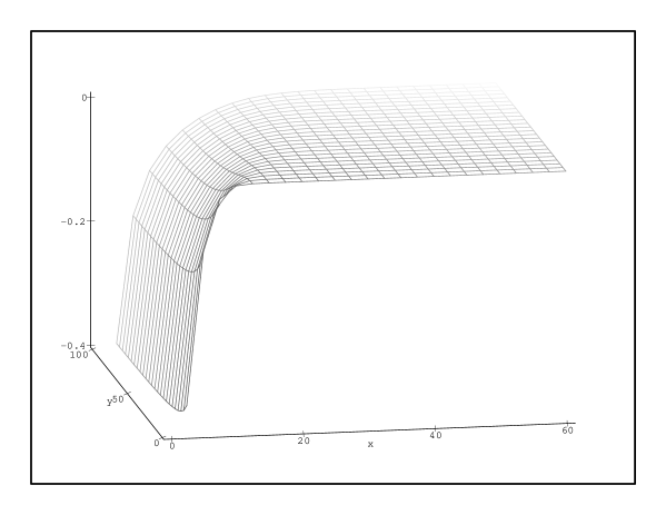
FIG. 1.: The short-range part $v^{(s)}$ of the $-1/x$ attractive Coulomb potential.

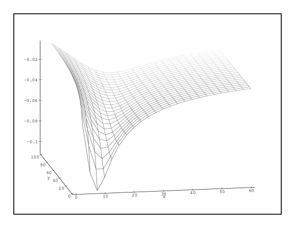
FIG. 2.: The long range part $v^{(l)}$ of the $-1/x$ attractive Coulomb potential.

FIG. 3.: Analytic structure of $g_{x_{\alpha}}(z-z^{\prime})\;g_{y_{\alpha}}(z^{\prime})$ as a function of $z^{\prime}$ with $z=E+{\mathrm{i}}\varepsilon$, $E<0$, $\varepsilon>0$. The contour $C$ encircles the continuous spectrum of $h_{y_{\alpha}}$. A part of it, which goes on the unphysical Riemann-sheet of $g_{y_{\alpha}}$, is drawn by broken line.

REFERENCES

• [1] J. V. Noble, Phys. Rev. 161, 945 (1967).
• [2] L. D. Faddeev and S. P. Merkuriev, Quantum Scattering Theory for Several Particle Systems (Kluwer, Dordrecht,1993).
• [3] Z. Papp, Phys. Rev. C 55, 1080 (1997).
• [4] Z. Papp and W. Plessas, Phys. Rev. C 54, 50 (1996).
• [5] Z. Papp, I. N. Filikhin and S. L. Yakovlev, to be published in Few-Body Systems, nucl-th/9909083.
• [6] Z. Papp, Few-Body Systems, 24 263 (1998).
• [7] V. Vanzani, Few-Body Nuclear Physics, (IAEA Vienna), 57 (1978).
• [8] E. O. Alt, P. Grassberger, and W. Sandhas, Nucl. Phys. B 2, 167 (1967).
• [9] W. Glöckle, Nucl. Phys. A141, 620 (1970); ibid. A158, 257 (1970).
• [10] S. L. Yakovlev, Theor. Math. Phys. 107, 835 (1996).
• [11] Z. Papp, J. Phys.  A 20, 153 (1987).
• [12] Z. Papp, Phys. Rev. C 38, 2457 (1988).
• [13] Z. Papp, Phys. Rev. A 46, 4437 (1992).
• [14] B. Kónya, G. Lévai, and Z. Papp, Phys. Rev. C 61, 034302 (2000).
• [15] M. Rotenberg, Ann. Phys. (N.Y.) 19, 262 (1962); Adv. At. Mol. Phys. 6, 233 (1970).
• [16] B. Kónya, G. Lévai, and Z. Papp, J. Math. Phys. 38, 4832 (1997).
• [17] L. Lorentzen and H. Waadeland, Continued Fractions with Applications (Noth-Holland, Amsterdam, 1992).
• [18] R. Balian and E. Brézin, Nuovo Cim.  B 2, 403 (1969).
• [19] W. Sandhas, Few-Body Nuclear Physics, (IAEA Vienna), 3 (1978).
• [20] A. A. Kvitsinsky, A. Wu, and C.-Y. Hu, J. Phys. B: At. Mol. Opt. Phys. 28 275 (1995).
• [21] A. K. Bhatia, A. Temkin, R. J. Drachman, and H. Eiserike, Phys. Rev. A 3, 1328 (1971).
• [22] F. S. Levin and J. Shertzer, Phys. Rev.  Lett. 61, 1089 (1988).
• [23] A. A. Kvitsinsky, J. Carbonell, and C. Gignoux, Phys. Rev. A 51, 2997 (1995).
• [24] C.-Y. Hu, Phys. Rev. A 59, 4813 (1999).