On a universal photonic tunnelling time

Abstract

We consider photonic tunnelling through evanescent regions and obtain general analytic expressions for the transit (phase) time $\tau$ (in the opaque barrier limit) in order to study the recently proposed “universality” property according to which $\tau$ is given by the reciprocal of the photon frequency. We consider different physical phenomena (corresponding to performed experiments) and show that such a property is only an approximation. In particular we find that the “correction” factor is a constant term for total internal reflection and quarter-wave photonic bandgap, while it is frequency-dependent in the case of undersized waveguide and distributed Bragg reflector. The comparison of our predictions with the experimental results shows quite a good agreement with observations and reveals the range of applicability of the approximated “universality” property.

]

I Introduction

In recent times, some photonic experiments [1]-[6] dealing with evanescent mode propagation have drawn some attention because of their intriguing results. All such experiments have measured the time required for the light to travel through a region in which only evanescent propagation occurs, according to classical Maxwell electrodynamic. If certain conditions are fulfilled (i.e. in the limit of opaque barriers), the obtained transit times are usually shorter than the corresponding ones for real (not evanescent) propagation through the same region. Due to the experimental setups, this has been correctly interpreted in terms of group velocities [7] greater than $c$ inside the considered region. Although there has been some confusion in the scientific community, leading also to several different definitions of the transit time [8], these results are not at odds with Einstein causality since, according to Sommerfeld and Brillouin [9], the front velocity rather than the group velocity is relevant for this. Waves which are solutions of the Maxwell equations always travel in vacuum with a front velocity equal to $c$ while, in certain conditions, their phase and group velocities can be different from $c$ [10]. It is worthwhile to observe that the quoted experiments are carried out studying different phenomena (undersized waveguide, photonic bandgap, total internal reflection) and exploring different frequency ranges (from optical to microwave region).
The interest in such experiments is driven by the fact that evanescent mode propagation through a given region can be viewed as a photonic tunnelling effect through a “potential” barrier in that region. This has been shown, for example, in Ref. [11] using the formal analogy between the (classical) Helmholtz wave equation and the (quantum mechanical) Schrödinger equation (see also Ref. [12]). In this respect, the photonic experiments are very useful to study the question of tunnelling times, since experiments involving charged particle (e.g. electrons) are not yet sensible enough to measure transit times due to some technical difficulties [13].
From an experimental point of view, the transit time $\tau$ for a wave-packet propagating through a given region is measured as the interval between the arrival times of the signal envelope at the two ends of that region whose distance is $D$. In general, if the wave-packet has a group velocity $v_{g}$, this means that $\tau=D/v_{g}$. Since $v_{g}=d\omega/dk$ ($k$ wave-vector, $\omega$ angular frequency), then we can write [14]:

$$\tau\;=\;\frac{d\phi}{d\omega}~{}~{}~{},$$ (1)

where $d\phi\,=\,D\,dk$ is the phase difference acquired by the packet in the considered region. The above argument works as well for matter particles in quantum mechanics, changing the role of angular frequency and wave-vector into the corresponding ones of energy and momentum through the Planck - de Broglie relations.
However, difficulties arise when we deal with tunnelling times, since inside a barrier region the wave-vector (or the momentum) is imaginary, and hence no group velocity can be defined. As a matter of fact, different definitions of tunnelling time exist. While we refer the read to the quoted literature [8], here we use the simple definition of phase time which coincides with Eq. (1). In fact, although $v_{g}$ seems meaningless in this case, nevertheless Eq. (1) is meaningful also for evanescent propagation. The adopted point of view takes advantage of the fact that experimental results [1]-[6] seem to confirm the definition of phase time for the tunnelling transit time.
Recently, Haibel and Nimtz [6] have noted that, regardless of the different phenomena studied, all experiments have measured photonic tunnelling times which are approximately equal to the reciprocal of the frequency of the radiation used in the given experiment. Such a “universal” behaviour is quite remarkable in view of the fact that, although photonic barrier traversal takes place in all the quoted experiments, nevertheless the boundary conditions are peculiar of each experiment.
In the present paper we carefully study the proposed universality starting from a common feature of tunnelling phenomena and, in the following section, derive a general expression for the transit (phase) time. Different experiments manifest themselves into different dispersion relations for the barrier region. We then analyze each peculiar experiment in Sects. III,IV,V and compare theoretical predictions with experimental observations. Finally, in Sect. VI, we discuss our results and give conclusions.
Note that, differently from other possible analysis (see, for example, the comparison with a photonic bandgap experiment in [15]), we deal with only tunnelling times, which have been directly observed, and not with velocities which, in the present case, are derived from transit times.

II Phase time and dispersion relation

In this paper we study one-dimensional problems or, more in general, phenomena in which evanescent propagation takes place along one direction, say $z$. Let us then consider a particle or a wave-packet moving along the $z$-axis entering in a region $[0,a]$ with a potential barrier $V(z)$ or a refractive index $n(z)$, as depicted in Figure 1. The energy/frequency of the incident particle/wave is below the maximum of the potential or cutoff frequency. For all experiments we’ll consider, the barrier can be modelled as a square one, in which $V(z)$ or $n(z)$ is constant in regions I,II,III but different from one region to another. We also assume that $V(z)$ or $n(z)$ is equal in I and III and take this value as the reference one.

FIG. 1.: A barrier potential $V(z)$ for a particle or a barrier refractive index $n(z)$ for an electromagnetic wave.

The propagation of the particle/wave through the barrier is described a by a scalar field $\psi$ representing the Schrödinger wave function in the particle case or some scalar component of the electric or magnetic field in the wave case. (The precise meaning of $\psi$ in the case of wave propagation depends on the particular phenomenon we consider. However, the aim of this paper is to show that a common background for all tunnelling phenomena exist). Given the formal analogy between the Schrödinger equation and the Helmholtz equation [11], [12], this function takes the following values in regions I,II,III, respectively:

$$\psi_{I} = e^{ikz}\,+\,R\,e^{-ikz}$$ (2)

$$\psi_{II} = A\,e^{-\chi z}\,+\,B\,e^{\chi z}$$ (3)

$$\psi_{III} = T\,e^{ik(z-a)}~{}~{}~{},$$ (4)

where $k$ and $k_{2}=i\chi$ are the wave-vectors ($p=\hbar k$ is the momentum) in regions I (or III) and II, respectively. Note that we have suppressed the time dependent factor $e^{i\omega t}$. Obviously, the physical field is represented by a wave-packet with a given spectrum in $\omega$:

$$\psi(z,t)\;=\;\int\,d\omega\,\eta(\omega)\,e^{i(kz-\omega t)}~{}~{}~{}.$$ (5)

where $\eta(\omega)$ is the envelope function. Keeping this in mind we use, however, for the sake of simplicity, the simple expressions in Eqs. (2), (3), (4). Furthermore, for the moment, we disregard the explicit expression fro $k$ and $\chi$ in terms of the angular frequency $\omega$ (or the relation between $p$ and $E=\hbar\omega$). As well known, the coefficients $R,T,A,B$ can be calculated from the matching conditions at interfaces:

$$\psi_{I}(0)\;=\;\psi_{II}(0)~{}~{}~{}~{} ~{}~{}~{}~{}\psi_{II}(a)\;=\;\psi_{III}(a)$$ , (6)

$$\psi_{I}^{\prime}(0)\;=\;\psi_{II}^{\prime}(0)~{}~{}~{}~{} ~{}~{}~{}~{}\psi_{II}^{\prime}(a)\;=\;\psi_{III}^{\prime}(a)~{}~{}~{},$$ , (7)

where the prime denotes differentiation with respect to $z$. Substituting Eqs. (2), (3), (4) into (6), (7) we are then able to find $R,T,A,B$ and thus the explicit expression for the function $\psi$. Here we focus only on the transmission coefficient $T$; its expression is as follows:

$$T\;=\;\left[1\,-\,r^{2}\,e^{-2\chi a}\right]^{-1}\,\left(1\,-\,r^{2}\right)\,e^{-\chi a}$$ (8)

with:

$$r\;=\;\frac{\chi+ik}{\chi-ik}~{}~{}~{}.$$ (9)

The interesting limit is that of opaque barriers, in which $\chi a\gg 1$. All photonic tunnelling experiments have mainly dealt with this case, in which “superluminal” propagation is predicted [16]. Taking this limit into Eq. (8) we have:

$$T\;\simeq\;2\,\left[1\,-\,i\,\frac{k^{2}-\chi^{2}}{2k\chi}\right]^{-1}\,e^{-\chi a}~{}~{}~{}.$$ (10)

The quantity $\phi$ in Eq. (1), relevant for the tunnelling time, is just the phase of $T$:

$$\phi\;\simeq\;\arctan\,\frac{k^{2}-\chi^{2}}{2k\chi}~{}~{}~{}.$$ (11)

The explicit evaluation of $\tau$ in Eq. (1) depends, clearly, from the dispersion relations $k=k(\omega)$ and $\chi=\chi(\omega)$. However, by substituting Eq. (11) into (1) we are able to write:

$$\tau\;=\;2\,\left[1\,+\,\left(\frac{k}{\chi}\right)^{2}\right]^{-1}\,\frac{d~{}}{d\omega}\,\frac{k}{\chi}~{}~{}~{},$$ (12)

showing that $\tau$ depends only on the ratio $k/\chi$. We can also obtain a particularly expressive relation by introducing the quantities:

$$\frac{k_{1}}{v_{1}}\;=\;k\,\frac{dk}{d\omega}~{}~{}~{}~{}~{},~{}~{}~{}~{}~{}\frac{k_{2}}{v_{2}}\;=\;-\,\chi\,\frac{d\chi}{d\omega}~{}~{}~{}.$$ (13)

In fact, in this case we get:

$$\tau\;=\;\frac{2}{\chi k}\,\left[\frac{\chi^{2}}{k^{2}+\chi^{2}}\,\frac{k_{1}}{v_{1}}\,+\,\frac{k^{2}}{k^{2}+\chi^{2}}\,\frac{k_{2}}{v_{2}}\right]~{}~{}~{}.$$ (14)

Note that while $k_{1}$ and $k_{2}$ are the real or imaginary wave-vectors in regions I (or III) and II, $v_{1}$ and $v_{2}$ represent the “real” or “imaginary” group velocities in the same regions. Obviously, an imaginary group velocity (which is the case for $v_{2}$) has no physical meaning, but we stress that in the physical expression for the time $\tau$ in (14) only the ratio $k_{2}/v_{2}$ enters, which is a well-defined real quantity.
Equations (12) and (14) are very general ones (holding in the limit of opaque barriers): they apply to all tunnelling phenomena. It is nevertheless clear that peculiarities of a given experiment enter in $\tau$ only through the dispersion relations $k=k(\omega)$ and $\chi=\chi(\omega)$ or, better, $k(\omega)/\chi(\omega)$.
As an example of application of the obtained general formula, we here consider the case of tunnelling of non relativistic electrons with mass $m$ through a potential square barrier of height $V_{0}$. (In the next sections we then study in detail the three types of experiment already performed). The electron energy is $E=\hbar\omega$ (with $E<V_{0}$) while the momenta involved in the problem are $p=\hbar k$ and $iq=\hbar k_{2}=i\hbar\chi$. In this case, the dispersion relations read as follows:

$$k = \sqrt{\frac{2m\,\omega}{\hbar}}$$ (15)

$$\chi = \sqrt{\frac{2m(V_{0}-\hbar\omega)}{\hbar^{2}}}$$ (16)

and thus:

$$\frac{k}{\chi}\;=\;\sqrt{\frac{\hbar\omega}{V_{0}-\hbar\omega}}~{}~{}~{}.$$ (17)

By substituting into Eq. (12) we immediately find:

$$\tau\;=\;\frac{\hbar}{\sqrt{E(V_{0}-E)}}\;=\;\frac{1}{\hbar}\;\frac{2m}{\chi k}~{}~{}~{}.$$ (18)

FIG. 2.: Frustrated total internal reflection in a double prism.

III Total internal reflection

The first photonic tunnelling phenomenon we consider is that of frustrated total internal reflection [17]. This is a two-dimensional process, but tunnelling proceeds only in one direction. With reference to Figure 2, a light beam impinges from a dielectric medium (typically a prism) with index $n_{1}$ onto a slab with index $n_{2}<n_{1}$. If the incident angle is greater than the critical value $\theta_{c}=\arcsin n_{2}/n_{1}$, most of the beam is reflected while part of it tunnels through the slab and emerges in the second dielectric medium with index $n_{1}$. Note that wave-packets propagate along the $x$ direction, while tunnelling occurs in the $z$ direction.
The wave-vectors $k_{1},k_{2}$ in regions I (or III) and II satisfy:

$$k_{1}^{2} = k_{x}^{2}\,+\,k^{2}$$ (19)

$$k_{2}^{2} = k_{x}^{2}\,-\,\chi^{2}~{}~{}~{},$$ (20)

where $k_{x}$ is the $x$ component of $k_{1}$ or $k_{2}$ and $k,\chi$ are as defined in the previous section. The dispersion relations in regions I (or III) and II are, respectively:

$$k_{1} = \frac{\omega}{c}\,n_{1}$$ (21)

$$k_{2} = \frac{\omega}{c}\,n_{2}~{}~{}~{}.$$ (22)

These equations also define the introduced quantities:

$$v_{1} = \frac{c}{n_{1}}$$ (23)

$$v_{2} = \frac{c}{n_{2}}~{}~{}~{}.$$ (24)

It is now very simple to obtain the tunnelling time in the opaque barrier limit for this process; in fact, by substituting Eqs. (21)-(24) into Eq. (14) we find:

$$\tau\;=\;\frac{1}{\omega}\,\frac{2k_{x}^{2}}{\chi k}~{}~{}~{}.$$ (25)

Furthermore, using the obvious relations:

$$k_{x} = k_{1}\,\sin\theta\;=\;\frac{\omega}{c}\,n_{1}\,\sin\theta$$ (26)

$$k = k_{1}\,\cos\theta\;=\;\frac{\omega}{c}\,n_{1}\,\cos\theta$$ (27)

$$\chi = \sqrt{k_{1}^{2}\,\sin^{2}\theta\,-\,k_{2}^{2}}\;=\;\frac{\omega}{c}\,\sqrt{n_{1}^{2}\,\sin^{2}\theta\,-\,n_{2}^{2}}~{}~{}~{},$$ (28)

we finally get:

$$\tau\;=\;\frac{1}{\nu}\,\frac{n_{1}\,\sin^{2}\theta}{\pi\,\cos\theta\,\sqrt{n_{1}^{2}\,\sin^{2}\theta\,-\,n_{2}^{2}}}~{}~{}~{}.$$ (29)

This formula can be directly checked with experiments. However, we firstly observe the interesting feature of this expression which does satisfy the property pointed out by Haibel and Nimtz [6]. In fact, the time $\tau$ in Eq. (29) is just given, apart from a numerical factor depending on the geometry and construction of the considered experiment, by the reciprocal of the frequency of the radiation used. In a certain sense, the numerical factor can be regarded as a “correction” factor to the “universality” property of Haibel and Nimtz.
Several experiments measuring the tunnelling time in the considered process have been performed [3].
In the experiment carried out by Balcou and Dutriaux [3], two fused silica prisms with $n_{1}=1.403$ and an air gap ($n_{2}=1$) are used. They employed a gaussian laser beam of wave-length $3.39\,\mu m$ with an incident angle $\theta=45.5^{o}$. Using these values into Eq. (29) we predict a tunnelling time of $36.8\,fs$, to be compared with the experimental result of about $40\,fs$. As we can see, the agreement is good and the “correction” factor in (29) is quite important for this to occur (compare with the Haibel and Nimtz prediction of $11.3\,fs$).
In the measurements by Mugnai, Ranfagni and Ronchi [3], the microwave region is explored, with a signal whose frequency is in the range $9\div 10\,GHz$. They used two paraffin prisms ($n_{1}=1.49$) with an air gap ($n_{2}=1$), while the incidence angle is about $60^{o}$. For this experiment we predict a tunnelling time of $87.2\,ps$, while the experimental result is $87{\pm}7\,ps$ .
Finally, we consider the recent experiment performed by Haibel and Nimtz [6] with a microwave radiation at $\nu=8.45\,GHz$ and two perspex prisms ($n_{1}=1.605$) separated by an air gap ($n_{2}=1$). For an incident angle of $45^{o}$, from (29) we predict $\tau=80.8\,ps$. The observed experimental result is, instead, $117{\pm}10\,ps$. In this case, the agreement is not very good (while, dropping the “correction” factor, Haibel and Nimtz find a better agreement); probably this is due to the fact that the condition of opaque barrier is not completely fulfilled.

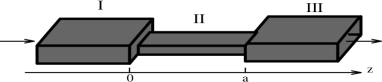
FIG. 3.: A waveguide with an undersized region.

IV Undersized waveguide

Let us now consider propagation through undersized rectangular waveguides as observed in [1]. Also in this case, evanescent propagation proceeds along one direction (say $z$) and the results obtained in Sect. II may apply. With reference to Figure 3, a signal propagating inside a “large” waveguide at a certain point undergoes through a “smaller” waveguide for a given distance $a$. As well known [18], the signal propagation inside a waveguide is allowed only for frequencies higher than a typical value (cutoff frequency) depending on the geometry of the waveguide. In the considered setup, the two differently sized waveguides I (or III) and II have, then, different cutoff frequencies (the first one, $\omega_{1}$, is smaller than the second one, $\omega_{2}$), and we consider the propagation of a signal whose frequency (or range of frequencies) is larger than $\omega_{1}$ but smaller than $\omega_{2}$: $\omega_{1}<\omega<\omega_{2}$. In such a case, in the region $0<z<a$ only evanescent propagation is allowed and, thus, the undersized waveguide acts as a barrier for the photonic signal. With the same notation of Sect. II, the dispersion relations in the large and small waveguide are, respectively:

$$c\,k = \sqrt{\omega^{2}\,-\,\omega_{1}^{2}}$$ (30)

$$c\,\chi = \sqrt{\omega_{2}^{2}\,-\,\omega^{2}}~{}~{}~{},$$ (31)

so that:

$$\frac{k}{\chi}\;=\;\sqrt{\frac{\omega^{2}\,-\,\omega_{1}^{2}}{\omega_{2}^{2}\,-\,\omega^{2}}}~{}~{}~{},$$ (32)

By substituting this expression into Eq. (12), we immediately find the tunnelling time in the regime of opaque barrier ($\chi a\gg 1$):

$$\tau\;=\;\frac{1}{\nu}\,{\cdot}\,\frac{1}{\pi}\,\sqrt{\frac{\nu^{4}}{(\nu^{2}-\nu_{1}^{2})(\nu_{2}^{2}-\nu^{2})}}~{}~{}~{}.$$ (33)

On the contrary to what happens for tunnelling in total internal reflection setups, the coefficient of the term $1/\nu$ isn’t constant but depends itself on frequency. Thus, in the case of undersized waveguides, the assumed “universality” property of Haibel and Nimtz cannot apply in general; depending on the cutoff frequencies, it is only a partial approximate property for frequencies far way from the cutoff values (i.e. when the term in the square root does not strongly depend on $\nu$).
Let us now compare the prediction (33) with the experimental results obtained in [1]. In the performed experiment we have microwave radiation along waveguides whose cutoff frequencies are $\nu_{1}=6.56\,GHz$ and $\nu_{2}=9.49\,GHz$, respectively. The radiation frequencies are around $\nu=8.7\,GHz$, so that tunnelling phenomena occur in the undersized waveguide. By substituting these values into Eq. (33), we predict a tunnelling time of $128\,ps$, confronting the observed time of about $130\,ps$.
As it is evident, also for an undersized waveguide setup the theory matches quite well with experiments. Note that, despite of the rich frequency dependence in Eq. (33), the Haibel and Nimtz property also works quite well (although some correction needs), since the central frequency value of the radiation used in the experiment is far enough from the cutoff values.

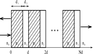
FIG. 4.: An ideal photonic bandgap device.

V Photonic bandgap

The last phenomenon we consider is that of light propagation through photonic bandgap materials. The ideal setup is depicted in Figure 4. Light impinges on a succession of thin plane-parallel films composed of $N$ two-layer unit cells of thicknesses $d_{1},d_{2}$ and constant, real refractive indices $n_{1},n_{2}$, embedded into a medium of index $n_{0}$. It is known [19] that such a multilayer dielectric mirror possesses a (one-dimensional) “photonic bandgap”, that is a range of frequencies corresponding to pure imaginary values of the wave-vector. In practice, it is the optical analog of crystalline solids possessing bandgaps. Increasing the number of periods will result in an exponential increase of the reflectivity, and thus the opaque barrier condition can be fulfilled. In general, the study of electromagnetic properties of such materials is very complicated, and the dispersion relation we need to evaluate the phase time in the proposed formalism is quite involved for physical situations. This study was performed analytically in [15] where the dispersion relation (and other useful quantities) was derived starting from the complex transmission coefficient of the considered barrier. It is, then, quite a meaningless issue to get the tunnelling time from the dispersion relation obtained from the transmission coefficient, while it is easier to have directly the phase time $\tau$ from Eq. (1), where $\phi$ is the phase of the complex transmission coefficient.

A Quarter-wave stack

We first consider the relevant case in which each layer is designed so that the optical path is exactly $1/4$ of some reference wave-length $\lambda_{0}$: $n_{1}d_{1}=n_{2}d_{2}=\lambda_{0}/4$. In such a case, $\lambda_{0}$ corresponds to the midgap frequency $\omega_{0}$ ($\lambda_{0}=2\pi c/\omega_{0}$). This condition is fulfilled in the considered experiments [2]. Finally, we further assume normal incidence of the light on the photonic bandgap material.
From [15] we then obtain the following expression for the transmission coefficient:

$$T\;=\;\left[\left(A\,C\,-\,B\right)\,+\,i\,A\,D\right]^{-1}~{}~{}~{},$$ (34)

where $A,B,C,D$ are real quantities given by:

$$A = \frac{\sin N\beta}{\sin\beta}$$ (35)

$$B = \frac{\sin(N-1)\beta}{\sin\beta}$$ (36)

$$C = a\,\cos\frac{\pi\omega}{\omega_{0}}\,+\,b$$ (37)

$$D = c\,\sin\frac{\pi\omega}{\omega_{0}}$$ (38)

$$a = \frac{1-r_{02}^{2}}{t_{02}t_{21}t_{12}}$$ (39)

$$b = \frac{r_{12}^{2}(r_{02}^{2}-1)}{t_{02}t_{21}t_{12}}$$ (40)

$$c = \frac{2r_{02}r_{12}-r_{02}^{2}-1}{t_{02}t_{21}t_{12}}$$ (41)

$$r_{ij} = \frac{n_{i}-n_{j}}{n_{i}+n_{j}}$$ (42)

$$t_{ij} = \frac{2n_{j}}{n_{i}+n_{j}}$$ (43)

$$\sin\beta\;=\;\frac{1}{t_{12}t_{21}}\,\sqrt{2r_{12}^{2}\,\left(\cos\frac{\pi\omega}{\omega_{0}}\,-\,1\right)\,+\,\sin^{2}\frac{\pi\omega}{\omega_{0}}}$$ (44)

($i,j=1,2$).The phase $\phi$ of the transmission coefficient thus satisfies:

$$\tan\phi\;=\;\frac{A\,D}{B\,-\,A\,C}~{}~{}~{}.$$ (45)

By substituting into Eq. (1), we finally get an analytic expression for the tunnelling time of light with frequency $\nu$ close to the midgap one $\nu_{0}$ for $N$ layers:

$$\tau\;=\;\frac{1}{\nu_{0}}\,{\cdot}\,\frac{1}{2}\,\frac{c\,\sinh N\theta}{\sinh(N-1)\theta\,+\,(b-a)\,\sinh N\theta}~{}~{}~{},$$ (46)

where $\theta$ is simply obtained from:

$$\sinh\theta\;=\;\frac{1}{2}\,\left(\frac{n_{2}}{n_{1}}\,-\,\frac{n_{1}}{n_{2}}\right)~{}~{}~{}.$$ (47)

Note that, although the tunnelling behaviour is quite different if the number of periods $N$ is an even or odd number (see, for example, [20]), the expression for the tunnelling time given in (46) (and also in (48)) is the same in both cases.
For future reference, we also report the appropriate formula for $N=k+(1/2)$ (integer $k$) multilayer dielectric mirrors. In practice, this models the case of a stratified medium whose structure has the form $n_{1}n_{2}n_{1}n_{2}\dots n_{1}n_{2}n_{1}$ (note, however, this is an approximation since, in general, $d/2$ is not equal to $a$). In such a case, Eq. (46) is just replaced by:

$$\tau\;=\;\frac{1}{\nu_{0}}\,{\cdot}\,\frac{1}{2}\,\frac{c\,\cosh N\theta}{\cosh(N-1)\theta\,+\,(b-a)\,\cosh N\theta}~{}~{}~{},$$ (48)

Let us observe that, similarly to total internal reflection, at midgap the time $\tau$ in Eq. (46) or (48) is again given by the reciprocal of the frequency times a “correction” constant factor.
We now analyze experimental results [2] in the light of our theoretical speculations.
In the experiment performed by Steinberg, Kwiat and Chiao, the authors used a quarter-wave multilayer dielectric mirror with a $(HL)^{5}H$ structure with a total thickness of $d=1.1\mu m$ attached on one side of a substrate and immersed in air. Here, $H$ represents a titanium oxide film with $n_{1}=2.22$, while $L$ is a fused silica layer with $n_{2}=1.41$. Thus, we have approximately $N=5+(1/2)$. As incident light, they employed a wave-packet centred at a wave-length $\lambda_{0}=702nm$, corresponding to the midgap frequency $\nu_{0}$ of about $427THz$. By substituting these numbers in our formula (48) we predict a tunnelling time $\tau=2.66\,fs$, corresponding to a delay time $\Delta t$, with respect to non tunnelling photons propagating at the speed of light the distance $d$, of $-1.01\,fs$. This has to be compared with the experimental result of $\Delta t=-(1.47{\pm}0.2)\,fs$. However, we point out that our analytical prediction is affected by two major approximations. The first one is, as already remarked, that the experimental sample is not really a $5+(1/2)$ periodic structure. A better approximation is achieved by using Eq. (46) with $N=6$ and subtracting the time required for travelling at the speed of light the quarter-wave thickness $d_{2}=\lambda_{0}/4n_{2}$. In this case we have $\tau=2.02\,fs$ or a delay time $\Delta t=-1.65\,fs$, which is in better agreement with the experimental result. Furthermore, in our analysis (leading to Eq, (46) or (48)) there is no room for considering an asymmetric structure (like the substrate-air one) in which the photonic bandgap material is embedded. This cannot be taken into account in an analytic framework, but has to be studied using numerical matrix transfer method which would give quite a good agreement with observations [15].
Finally, we consider the experiment carried out by Spielmann et al. [2] on alternated quarter-wave layers of fused silica $L$ and titanium dioxide $H$ having the structure of $(substrate)(HL)^{n}(air)$ with $N=3,5,7,9,11$. They used optical pulses of frequency $375$$THz$ corresponding to the midgap frequency of their photonic bandgap material. Obviously, increasing $N$ we have a better realization of opaque barrier condition. From Eq. (46) with $N=11$ (note, however, that for $N\geq 5$ the factor $\sinh(N-1)\theta/\sinh N\theta$ is almost constant) we have a tunnelling time of $2.98\,fs$ to be compared with the observed value of about $2.71\,fs$. We address the fact that, apart the presence of the asymmetric substrate-air structure which introduces some approximation as discussed above, in the considered experiment the incidence of the light on the sample is not normal, being $\approx 20^{o}$ the angle between the axis of the sample and the beam propagation direction. In this case, the described computations are only approximated ones and, again, the exact result can be obtained only through numerical implementation. Nevertheless, also within the limits of our calculations, the agreement between theory and experiment is quite good.
A final comment regards the predictions of the “universality” property proposed by Haibel and Nimtz. Neglecting the “correction” factor in Eq. (46) would yield the values of $\Delta t=-1.33\,fs$ and $\tau=2.67\,fs$ for the delay time in the Steinberg, Kwiat and Chiao experiment and the transit time for the Spielmann et al. experiment, respectively. In both cases, the agreement with the observed values seems better than our approximated predictions, showing that the presence of an asymmetric substrate-air structure (and the non normal incidence in the second experiment) pushes up the “correction” factor in Eq. (46).

B Distributed Bragg Reflector

We now relax the assumption of a quarter-wave stack $n_{1}d_{1}=n_{2}d_{2}=\lambda_{0}/4$ but, for simplicity, we consider only the case in which the photonic bandgap structure is embedded into a material whose refractive index $n_{0}$ is equal to that of one of the two layers of the periodic structure, that is $n_{0}=n_{2}$. We again assume normal incidence of the light on the photonic bandgap material. In this case the transmission coefficient $T$ and its phase $\phi$ have the expressions as in (34) and (45), where $A$,$B$ are given by (35), (36) and [15]:

$$C = a\,\cos\pi\,\Omega_{+}\,\omega\;-\;b\,\cos\pi\,\Omega_{-}\,\omega$$ (49)

$$D = -\,a\,\sin\pi\,\Omega_{+}\,\omega\;+\;b\,\sin\pi\,\Omega_{-}\,\omega$$ (50)

$$\Omega_{\pm}\;=\;\frac{n_{1}d_{1}\,{\pm}\,n_{2}d_{2}}{c}$$ (51)

$$\sin\beta\;=\;\frac{1}{t_{12}t_{21}}\,\sqrt{P\,+\,Q\,+\,R}$$ (52)

$$P = r_{12}^{4}\,\sin^{2}\pi\,\Omega_{-}\,\omega$$ (53)

$$Q = 2r_{12}^{2}\,\left(\cos\pi\,\Omega_{+}\,\omega\,\cos\pi\,\Omega_{-}\,\omega\,-\,1\right)$$ (54)

$$R = \sin^{2}\pi\,\Omega_{+}\,\omega$$ (55)

By substituting into Eq. (1) we obtain the tunnelling time relative to an $N$-layer structure:

$$\tau\;=\;\frac{1}{\nu}\,\frac{X-Y}{Z}$$ (56)

$$X = F\sin^{2}\beta\cos N\beta\sin N\beta$$ (57)

$$Y = G\left(\cos\beta\cos N\beta\sin N\beta-N\sin\beta\right)$$ (58)

$$Z = 2\,\sin\beta\left(D^{2}\sin^{2}N\beta+\sin^{2}\beta\cos^{2}N\beta\right)$$ (59)

$$F = a\,\Omega_{+}\,\omega\,\cos\pi\Omega_{+}\omega\,-\,b\,\Omega_{-}\,\omega\,\cos\pi\Omega_{-}\omega$$ (60)

$$G = a^{2}\,\Omega_{+}\,\omega\,\sin^{2}\pi\Omega_{+}\omega\,+\,b^{2}\,\Omega_{-}\,\omega\,\sin^{2}\pi\Omega_{-}\omega\,+$$ (61)

$$-\,2ab\,(\Omega_{+}+\Omega_{-})\,\omega\,\sin\pi\Omega_{+}\omega\,\sin^{2}\pi\Omega_{-}\omega$$ (62)

Note that, again, the formula above for $\tau$ holds both for even $N$ and for odd $N$.
The obtained expression for the tunnelling time can be directly tested by analyzing the experiment carried out by Mojahedi, Schamiloglu, Hegeler and Malloy [5]. In this experiment the authors used a (1D) photonic crystal composed of 5 polycarbonate sheets with refractive index $n_{1}=1.66$ and thickness $d_{1}=1.27\,cm$ separated by regions of air $n_{2}=1$ with thickness $d_{2}=4.1\,cm$. The bandgap was tuned to the main frequency component ($\nu=9.68\,GHz$) of the incident microwave pulse. By measuring both the signal travelling through the photonic bandgap structure and the one propagating in free space, the authors found that the pulse undergoing tunnelling has a delay time $\Delta t=-(440{\pm}20)\,ps$ with respect to the other signal. By using Eq. (56) with the above numbers we predict a tunnelling time of $320\,ps$ , corresponding to a delay time of $\Delta t=-438\,ps$, which is in excellent agreement with the reported experimental result.
We point out that, in this case, the simple $1/\nu$ law proposed by Haibel and Nimtz does not work, since it would predict a tunnelling time $\tau=103\,ps$ or $\Delta t=-655\,ps$. This can be easily explained by looking at Eq. (56). In fact, we immediately recognize that the “correction” factor in this equation is strongly frequency-dependent and, for the frequency of the light used in the considered experiment, it is sensibly bigger than one.

VI Conclusions

In this paper we have scrutinized the recently proposed [6] “universality” property of the photonic tunnelling time, according to which the barrier traversal time for photons propagating through an evanescent region is approximately given by the reciprocal of the photonic frequency, irrespective of the particular setup employed. To this end, the transit time in the relevant region, defined here as in Eq. (1), needs to be computed for the different explored phenomena, and in Sect. II we have given general expressions for this time in the opaque barrier limit. The peculiarities of a given photonic setup enter in these expression only through the dispersion relation relating the wave-vector and the frequency. More in detail, we have shown how the knowledge of the ratio between the wave-vectors in the barrier region and outside it, as a function of the photon frequency, is sufficient to evaluate the transit time $\tau$ in Eq. (12).
Several specific cases, corresponding to the different classes of experimentally investigated phenomena, have then been considered. In particular, in Sect. III we have studied light propagation in a setup in which the evanescent region is provided by total internal reflection, while in Sect. IV the propagation through undersized waveguides has been considered and, finally, in Sect. V the case of a photonic bandgap has been analyzed. The relevant results for the three mentioned phenomena are given in Eqs. (29), (33) and (46) or (56), respectively. As can be easily seen from these expressions, the frequency dependence of the tunnelling time for the cases of total internal reflection and quarter-wave photonic bandgap is just as predicted by the property outlined by Haibel and Nimtz [6], although we have derived a “correction” factor depending on the geometry and on the intrinsic properties of the sample (this factor is not far from unity). On the contrary, such a factor is frequency dependent for undersized waveguides and distributed Bragg reflectors, revealing a more rich dependence of $\tau$ on $\nu$ than the simple $1/\nu$ one (see Eq. (33)). We can then conclude that the “universality” property of Haibel and Nimtz is only an approximation, but it gives the right order of magnitude for the tunnelling time. This conclusion holds also for undersized waveguide propagation, provided that the photon frequency is far enough from the cutoff frequencies.

TABLE I.: Comparison between predicted and observed tunnelling times for several experiment (FTIR, UWG and PBG stands for frustrated total internal reflection, undersized waveguide and photonic bandgap, respectively). $\tau_{exp}$ is the experimental result while $\tau_{th}$ is our prediction as from Eqs. (29), (33) and (46) or (56). For reference to the Haibel and Nimtz property, we also report the value $1/\nu$.

Phenomenon	Experiment	$1/\nu$	$\tau_{th}$	$\tau_{exp}$
FTIR	Balcou et al. [3]	$11.3\,fs$	$36.8\,fs$	$\sim 40\,fs$
FTIR	Mugnai et al [3]	$100\,ps$	$87.2\,ps$	$87{\pm}7\,ps$
FTIR	Haibel et al. [6]	$120\,ps$	$81\,ps$	$117{\pm}10\,ps$
UWG	Enders et al. [1]	$115\,ps$	$128\,ps$	$\sim 130\,ps$
PBG($\lambda_{0}/4$)	Steinberg et al. [2]	$2.34\,fs$	$2.02\,fs$	$2.20{\pm}0.2\,fs$
PBG($\lambda_{0}/4$)	Spielmann et al. [2]	$2.67\,fs$	$2.98\,fs$	$\sim 2.71\,fs$
PBG	Mojahedi et al. [5]	$103\,ps$	$320\,ps$	$318{\pm}20\,ps$

We have then calculated the tunnelling times for the different existing experiments and compared the theoretical values with the observed ones. Results are summarized in Table 1, where we also report the Haibel and Nimtz prediction $1/\nu$. From these we can see that, in general, the agreement of our prediction with the experimental values is satisfactory. As pointed out in the previous section, the calculations performed here for photonic bandgap materials assume some approximations in treating the complex sample, which are nevertheless required to obtain analytical expressions. Our prediction then suffer of this and, in the case in which the setup is designed to verify the quarter-wave condition $n_{1}d_{1}=n_{2}d_{2}=\lambda_{0}/4$, the simple $1/\nu$ rule fits better with experiments while, for general photonic bandgap structures, the tunnelling time displays a very complicated dependence on frequency. In this last case, as well as in all other non photonic bandgap experiments, the “correction” factor introduced in this paper is quite relevant for the agreement with observations to be good.

- [1] A. Enders and G. Nimtz, J. Phys. I (France) 2 (1992) 1693.
- [2] A.M. Steinberg, P.G. Kwiat and R.Y. Chiao, Phys. Rev. Lett. 71 (1993) 708; Ch. Spielmann, R. Szipocs, A. Stingl and F. Krausz, Phys. Rev. Lett. 73 (1994) 2308; G. Nimtz, A. Enders and H. Spieker, J. Phys. I (France) 4 (1994) 565.
- [3] Ph. Balcou and L. Dutriaux, Phys. Rev. Lett. 78 (1997) 851; D. Mugnai, A. Ranfagni and L. Ronchi, Phys. Lett. A 247 (1998) 281; J.J. Carey, J. Zawadzka, D.A. Jaroszynski and K. Wynne, Phys. Rev. Lett. 84 (2000) 1431.
- [4] M. Mojahedi, E. Schamiloglu, K. Agi and K.J. Malloy, IEEE J. Quant. Electronics 36 (2000) 418.
- [5] M. Mojahedi, E. Schamiloglu, F. Hegeler and K.J. Malloy, Phys. Rev. E 62 (2000) 5758.
- [6] A. Haibel and G. Nimtz, Ann. Phys. (Leipzig) 10, Edition 8 (2001), e-print physics/0009044.
- [7] See the discussion in W. Heitmann and G. Nimtz, Phys. Lett. A 196 (1994) 154.
- [8] V.S. Olkhovsky and E. Recami, Phys. Report 214 (1992) 339 and Refs. therein.
- [9] A. Sommerfeld, ‘Vorlesungen über Theoretische Physik’, Band IV, Optik, Dieterichsche Verlagsbuchhhandlung (1950); L. Brillouin, Wave propagation and group velocity (Academic Press, New York, 1960).
- [10] S. Esposito, Phys. Lett. A 225 (1997) 203.
- [11] Th. Martin and R. Landauer, Phys. Rev. A 45 (1992) 2611; R. Chiao, P. Kwiat and A. Steinberg, Physica B 175 (1991) 257; A. Ranfagni, D. Mugnai, P. Fabeni and G. Pazzi, Appl. Phys. Lett. 58 (1991) 774.
- [12] V.S. Olkhovsky, E. Recami and J. Jakiel, preprint quant-ph/0102007.
- [13] P. Guèret, E. Marclay and H. Meier, Europhys. Lett. 3 (1987) 367; P. Guèret, A. Baratoff and E. Marclay, Solid State Commun. 68 (1988) 977; see also Th. Martin and R. Landauer in [11].
- [14] E. Merzbacher, Quantum Mechanics (Wiley, New York, 1970).
- [15] J.M. Bendickson, J.P. Dowling and M. Scalora, Phys. Rev. E 53 (1996) 4107.
- [16] T.E. Hartman, J. Appl. Phys. 33 (1962) 3427; J.R. Fletcher, J. Phys. C 18 (1985) L55.
- [17] A.K. Ghatak, M.R. Shenoy, I.C. Goyal and K. Thyagarajan, Opt. Commun. 56 (1986) 313; A.K. Ghatak and S. Banerjee, Appl. Optics 28 (1989) 1960 and Refs. therein.
- [18] J.D. Jackson, Classical Electrodynamics (Wiley, New York, 1975).
- [19] M. Born and E. Wolf, Principles of Optics (Pergamon, New York, 1980).
- [20] W. Yun-ping and Z. Dian-Lin, Phys. Rev. A 52 (1995) 2597; V. Laude and P. Tournois, J. Opt. Soc. Am. B 16 (1999) 194.