Self-adaptive exploration in evolutionary search

Abstract

• We address a primary question of computational as well as biological research on evolution: How can an exploration strategy adapt in such a way as to exploit the information gained about the problem at hand? We first introduce an integrated formalism of evolutionary search which provides a unified view on different specific approaches. On this basis we discuss the implications of indirect modeling (via a “genotype-phenotype mapping”) on the exploration strategy. Notions such as modularity, pleiotropy and functional phenotypic complex are discussed as implications.

  Then, rigorously reflecting the notion of self-adaptability, we introduce a new definition that captures self-adaptability of exploration: different genotypes that map to the same phenotype may represent (also topologically) different exploration strategies; self-adaptability requires a variation of exploration strategies along such a “neutral space”. By this definition, the concept of neutrality becomes a central concern of this paper.

  Finally, we present examples of these concepts: For a specific grammar-type encoding, we observe a large variability of exploration strategies for a fixed phenotype, and a self-adaptive drift towards short representations with highly structured exploration strategy that matches the “problem’s structure”.

Keywords

• Exploration, self-adaptability, evolvability, neutrality, modularity, pleiotropy, functional phenotypic complex.

1 Introduction

Typically, when a problem is given, the space of all potential solutions is too large to try all of them in reasonable time. If not making any further assumptions on the problem, there neither exists a preferable strategy to search for solutions. Usually though, one assumes that the problem is not notoriously arbitrary, that it has some “structure” and that there might exist some smart strategies to explore the space. More specifically, one hopes that one can draw information from the quality of previously explored solutions on how to choose new explorations. For example, when assuming some “continuity” of the problem, one may search further in regions of previously explored good solutions.

A more elaborated strategy is the following: Analyze the statistics of previously found solutions, find correlations between certain characters (parameters) of the solution and the solution’s quality, find mutual information between the characters of good solutions, etc., and exploit all this information to choose further explorations — in the hope that these findings really characterize the problem, that the problem is characterizable by such information. In essence, the latter approach will explore only a tiny part of $P$, strongly dependent on early explorations that have been successful. Found solutions may lay no claim to be globally optimal; they are a further development of early successful concepts.

The central questions become: How can we analyze the statistics of previously explored and evaluated solutions? How can we represent this gained information? How can we model an exploration strategy depending on this information?

One direct approach to these questions leads to statistical models of exploration. For example, a Bayesian network can encode the probability of future explorations (the exploration density) and is trained with previously successful solution parameters (as done by pelikan:00, see appendix A). In contrast, we will argue that the exploration strategy can be modeled by a mapping onto the solution space, a genotype-phenotype mapping. This means that a (simple) density on a base space (genotype) is lifted to the exploration density on the search space (phenotype). The implications of such an ansatz are far-reaching: An exploration density now exists on both, the base space and the search space. In both spaces notions as neighborhood or topology should be constituted only by the exploration density. In this respect, the genotype-phenotype mapping is a lift of (topological) structure from the base space to the search space.

To investigate the implications, we assume that the exploration density on the base space is one of independent random variables. Then, for a given mapping, we investigate the exploration density on the search space; in particular the correlations and mutual information between phenotypic variables. This structuredness of phenotypic exploration coherently implies notions as “modularity” and “functional phenotypic complex”. Concerning the adaption of this structure, we will argue for a self-adaptive mechanism, in place of a statistical analysis of characters of good solutions (as with the Bayesian ansatz). A major goal of this paper is formal and notational clarity of such issues.

The paper is organized as follows: The next section starts by introducing a general notation of evolutionary search. This notation emphasizes the role of the exploration density in the search space and, even more, the way of parameterization of this density. We call the latter “exploration model”. An important point of this section is that most evolutionary algorithms differ just by this exploration model. Since it distracts from the major line of this paper we moved this reinvestigation of existing evolutionary algorithms to appendix A.

In section 3 we introduce and formalize the idea of indirect modeling. Instead of parameterizing the exploration density directly on the search space, we introduce the additional base space, parameterize a simple density thereon, and lift this density on the search space. We compare this to the lift of a topological or metrical structure onto a manifold from a simple-structured base space. Notions as pleiotropy and functional phenotypic complex are discussed as implications of such a lift. We also relate the biological view on indirect modeling (here, via a genotype-phenotype mapping) and adaptive exploration to our formalism.

Section 4 begins by reflecting and criticizing the usual definition of self-adaptability. We introduce a new definition which is based on the notion of neutrality: Different genotypes that map to the same phenotype may represent (also topologically) different exploration densities. Thus, such genotypes may represent very different information and neutrality is not necessarily a form of redundancy as is often claimed. By this definition, neutrality becomes a central concern and we briefly review other research on this subject in order to argue for the plausibility of our interpretation.

Finally, in section 5 we exemplify all these concepts with a running system. Simulations show that the exploration density adapts to the problem structure by (self-adaptive) walks on neutral sets. In particular, the pair-wise mutual information between phenotypic variables resembles the modularity of the fitness function. We also observe and explain a drift towards short representations. The experiments are based on a grammar-type recursive encoding which is thoroughly motivated by the previously developed concepts.

2 The central role of the exploration model

The goal of this section is to show that the central concern of evolutionary search, esp. evolutionary algorithms, is the modeling of exploration. We will show that the main difference between specific evolutionary algorithms is their ansatz to model exploration.

Perhaps the most general idea of stochastic search, global random search, is described by zhigljavsky:91. The formal scheme of global random search reads:

1. Choose a probability distribution on the search space $P$.

2. Obtain points $s_{1}^{(t)},\dots,s_{\lambda}^{(t)}$ by sampling $\lambda$ times from this distribution. Evaluate the quality of these points.

3. According to a fixed (algorithm dependent) rule construct a new probability distribution on $P$.

4. Check some appropriate stopping condition; if the algorithm is not terminated, then substitute $t\leftarrow t+1$ and return to step (ii).

This concept is general enough to include also evolutionary algorithms. However, the formulation lacks to stress that the exploration density needs to be parameterized (and instead stresses the choice of update rule in step (iii)). We will stress the parameterization of exploration densities and call it the exploration model. It is this model that we focus on. We now formalize evolutionary search in analogy to global random search, but with different focus:

In general we assume that the task is to find an element $p$ in a search space $P$ which is “superior” to all other points in $P$. Here, superiority is defined in terms of a quality measure for the search problem at hand (usually a fitness function). If $P$ is too large to evaluate the quality of all $p\in P$, the strategy is to explore only a few points $(p_{1},..,p_{\lambda})$, evaluate their quality, and then try to extract information on where to perform further explorations. We capture this view on evolutionary search in an abstract formalism that is capable to unify the different specific approaches. Below, we exemplify each step of the scheme by embedding the Simple Genetic Algorithm (SGA) [VoseVose1999] in the formalism. See also figure 1.

Definition 1

(Evolutionary exploration)

1. The only information maintained for evolutionary search is a finite set of parameters $q^{(t)}\in Q$ that uniquely define an exploration density $M_{q^{(t)}}$ on $P$. Here, we call $M$ the exploration model, actually a map from $Q$ to the space $\Lambda$ of densities over $P$. In general, the variety $M_{Q}=\{M_{q}\,|\,q\in Q\}$ of representable densities is limited.

2. Given some parameters $q^{(t)}$, exploration starts by choosing $\lambda$ samples $s^{(t)}_{i=1..\lambda}$ of the exploration density. We use brackets to indicate this sampling:

   $$s^{(t)}=[M_{q^{(t)}}]_{\lambda}\in P^{\lambda}\;.$$ (1)

   Here and in the following, we disregard the possibility of elitists. Taking them into account would require to append selected points $(p_{1},..,p_{\mu})$ of $P$ to $s^{(t)}$,

   $$s^{(t)}=[M_{q^{(t)}}]_{\lambda}\oplus(p_{1},..,p_{\mu})\in P^{\mu+\lambda}\;.$$ (2)

3. We require the existence of an evaluation $E:\,P^{\lambda}\to\Lambda$ which maps the exploration sample $(s_{1},..,s_{\lambda})$ to a density over $P$ with support $\{s_{1},..,s_{\lambda}\}$. This evaluation is applied to our exploration points:

   $$E_{s^{(t)}}=E\big{(}[M_{q^{(t)}}]_{\lambda}\big{)}\in\Lambda\;.$$ (3)

   One should interpret $E$ as “density of quality” rather than a probability density.

4. Finally, there exists an update operator

   $$A:\,q^{(t)}\times E_{s^{(t)}}\mapsto q^{(t+1)}\;.$$ (4)

   In general, this operator is supposed to exploit the information in $E_{s^{(t)}}$.

Example

(The Simple Genetic Algorithm)

1. The SGA (without crossover) is a typical example of population-based modeling: $q^{(t)}=(p_{1},..,p_{\mu})\in P^{\mu}$ is a discrete population and $\tilde{M}_{p_{i}}$ specifies the offspring density for each single individual. We call $\tilde{M}_{p_{i}}$ exploration kernels. The total exploration density reads

   $$M_{q}=\frac{1}{\mu}\sum_{i=1}^{\mu}\tilde{M}_{p_{i}}\;.$$ (5)

   We note that the key feature of population-based modeling is its capacity to represent multi-modal exploration densities.

2. In the SGA, $s^{(t)}$ are new offsprings. The algorithms does not explicitly construct the complete exploration density $M_{q^{(t)}}$; rather, the drawing of mutations for each individual resembles a sampling of the exploration kernels.

3. For the SGA, evaluation is proportional to a given fitness function.

4. The update rule of the SGA can be written as

   $$q^{(t+1)}=\Big{[}E\big{(}[M_{q^{(t)}}]_{n}\big{)}\Big{]}_{n}\;.$$ (6)

   In words: From the parent population $q^{(t)}$ generate $n$ offsprings $[M_{q^{(t)}}]_{n}$, evaluate their fitness and select $n$ new individuals by sampling their evaluation.

One might assume that evolutionary algorithms mostly differ with respect to the update rule. However, we claim that the choice of the exploration model is crucial and that, given such a model, two generic update operators are canonical and widely in use:

Definition 2

(Adopting and approaching updates)

• It is the adopting update to choose the update operator such that $M_{q^{(t+1)}}$ is a best possible approximation of $E_{s^{(t)}}$ within the model class $M_{Q}$ (with respect to some chosen metric $D$ on $\Lambda$):

  $$q^{(t+1)}=\mathrm{arg}\underset{q}{\mathrm{min}}\,D(M_{q}\!:\!E_{s^{(t)}})\;.$$ (7)

  We will abbreviate this formula by using the simplified notation $A=M^{-1}$:

  $$q^{(t+1)}=M^{-1}(E_{s^{(t)}})\;.$$ (8)

  Second, many algorithms realize not an adopting but rather an approaching update by slowly adapting $q^{(t)}$. Here, the parameters must be continuous. The generic update rule reads

  $$q^{(t+1)}=(1-\alpha)\;q^{(t)}+\alpha\;M^{-1}(E_{s^{(t)}})\;,$$ (9)

  for some constant $\alpha\in[0,1]$.

Example

(Update operator of the SGA)

• The update operator of the SGA is strongly related to the adopting update: The sampling $[E_{s^{(t)}}]_{n}$ of the evaluation density can be interpreted as “finding new parameters $q^{(t+1)}$ that approximate $E_{s^{(t)}}$ in the population-based model”. The quality of this approximation is reflected by the sampling error.

Both of these canonical update operators are derived from $M^{-1}$. Thus, when we show that most existing evolutionary algorithms realize these operators, then we stress the importance of the choice of exploration model. Note that any algorithm, when embedded in the upper formalism, is uniquely characterized by the choice of model $M$, the update operator $A$ (eventually derived form $M$), the evaluation $E$ (given at hand) and the sampling size $\lambda$.

It is, of course, possible to think of exceptions that cannot be embedded in this formalism. However, in appendix A we show how the formalism allows an embedding of – and a unified view on – very different state-of-the-art evolutionary algorithms. Indeed, those evolutionary algorithms mainly differ with respect to their exploration model.

Figure 1: The general scheme of evolutionary search.

3 An indirect model of exploration

After we stressed the importance of exploration modeling we concentrate on the specific case of modeling defined as follows:

Definition 3

(Indirect exploration modeling)

• To model an exploration density over $P$, introduce a base space $G=X^{n}$ and a base density $M^{G}_{q}$ over $G$ such that the variables $x\in X$ are independent with respect to $M^{G}_{q}$. Then, introduce a GP-map $h:\,G\to P$ that induces the exploration density $M_{q}=M^{G}_{q}\circ h^{-1}$ over $P$. Here, $h^{-1}(p)\subset G$ is a subspace of $G$ called neutral space of $p\in P$; and $M^{G}_{q}\big{[}h^{-1}(p)\big{]}$ is evaluated via integration. The class of allowed GP-maps and base densities limits this model $M$. The triplet $(G,h,M^{G})$ is also referred to as coding.

In the following, in order to refer to their biological interpretations, we will also use the names phenotype space for the search space $P$, genotype space for the base space $G$, and phenotype-genotype mapping for $h$.

Also, we call the independent variables $x\in X$ genes and say we introduce genes on $P$ when introducing such a GP-map and stressing the introducing of a representation via independent variables. This can be seen in analogy to the introduction of local coordinates on a manifold by a local map from a base space of (Cartesian) variables. There is, however, a crucial difference: The map $h$ does not need to be one-to-one. If $h$ is non-injective, there exist different genotypes $g_{i}$ that map to the same phenotype. Then there exist different neighborhoods $U_{g_{i}}$ that map to eventually different neighborhoods of the same phenotype. This change of neighborhood is of major interest. It allows a variability of exploration. The next section will address this important issue in detail.

As an example for indirect modeling, note that the CMA (see appendix A) may be interpreted as indirect modeling: it restricts the class of GP-maps to affine transformations; the translational part is encoded in the population’s center of mass and the linear part is encoded in the covariance matrix; the base space is $G=\mathbb{R}^{n}$ with normal density ${\cal N}(0,1)$.

3.1 Characters of indirect exploration: Pleiotropy, mutual information, lift of topology, neutrality

The introduction of a GP-map leads to some straightforward definitions and notions. We use this section to briefly introduce some.

Pleiotropy.

In a biological context one may define pleiotropy as “the phenomenon of one gene being responsible for or affecting more than one phenotypic characteristic”. Our previous definitions allow to translate this notion into our formalism: Genes are independent (with respect to the base density) variables of $G$. One gene affecting more than one variable of $P$ means that the change of one variable in $G$ leads to the change of many variables in $P$. Thus pleiotropy means that the base density of independent variables is mapped on an exploration density of non-independent variables; pleiotropy may be measured by the correlatedness of variables of $P$ with respect to the exploration density. We refer to this also as structure of the exploration density. In particular, we will measure pleiotropy as the mutual information contained in the exploration density.

Population-based indirect modeling.

Population-based modeling was defined in section 2. We briefly clarify notations in the indirect modeling case: The parameters $q\in Q$ are a population $(g_{1},..,g_{\mu})\in G^{\mu}$ on the base space and the exploration kernels $\tilde{M}^{G}_{g_{i}}$ are such that the total exploration density reads:

$$M_{q} =M^{G}_{q}\circ h^{-1}=\Big{[}\frac{1}{\mu}\sum_{i=1}^{\mu}\tilde{M}^{G}_{g_{i}}\Big{]}\circ h^{-1}=\frac{1}{\mu}\sum_{i=1}^{\mu}\Big{[}\tilde{M}^{G}_{g_{i}}\circ h^{-1}\Big{]}=:\frac{1}{\mu}\sum_{i=1}^{\mu}\tilde{M}_{g_{i}}\;.$$ (10)

Lift of topology.

For population-based modeling, the exploration kernels associate a density of offsprings to each individual. Form a topological point of view, this defines a neighborhood (of most probable offsprings) for each individual, referred to as variational topology.

In the case of indirect modeling, the kernels $\tilde{M}^{G}_{g}$ on the base space are lifted to kernels $\tilde{M}_{g}=\tilde{M}^{G}_{g}\circ h^{-1}$ on the search space. This means a lift of topology.

Neutrality.

The possibility of a non-injective GP-map $h$ automatically leads to the definition of neutrality. In particular we define $h^{-1}(p)$ as the neutral set of $p\in P$. Further, the neutral degree of $g\in G$ is defined as the probability

$$\tilde{M}_{g}[h(g)]=\tilde{M}^{G}_{g}[h^{-1}\!\circ\!h(g)]\;.$$ (11)

This reads: Take some individual $g\in G$ and let $N=h^{-1}\!\circ\!h(g)$ be the neutral space “around” $g$. Now measure the probability $\tilde{M}^{G}_{g}[N]$ for landing in this neutral set when exploring from $g$.

Such measures are thoroughly discussed by schuster:96 and fontana:98 (see also section 4.1). However, in these publications, the variational topology rather than the probability is emphasized. For completeness we append: Let neighborhoods be defined in $G$ and let $B_{r}(g)$ be the $r$-ball around $g$ in $G$ (those points linked to $G$ by at least one chain of no more than $r$ neighbors). We call the maximal connected component $N_{g}\subset h^{-1}\!\circ\!h(g)$ with $g\in N_{g}$ neutral network of $g\in G$ and define:

$$|h^{-1}(h(g))\cap B_{1}(g)| g\in G$$ neutral degree of (12)

3.2 Indirect exploration modeling in biology

One may argue that algorithms as discussed in appendix A are hardly plausible in nature and thus without relevance for biology. What mechanisms should keep track of dependencies in nature, model distributions by storing a Bayesian network or a covariance matrix, and how should such knowledge be taken into account when creating new offsprings?

Nevertheless, a biologist may in principle ask the same questions; we refer to wagner:96: How comes that some phenotypic characters are obviously correlated and others are not? How comes that a single gene in Drosophila can trigger the expression of many others and thereby the growth of a whole eye at different places on the body? The existence of pleiotropy is obvious; are its specific mechanisms an accident, an unavoidability, or the result of evolutionary optimization? What is optimized when adapting pleiotropy?

The idea of Wagner and Altenberg is that in nature the genotype-phenotype mapping is adaptable and does adapt in such a way that pleiotropy between independent phenotypic characters is decreased (in order to allow for an unbiased, parallel search) while pleiotropy between correlated phenotypic characters may increase (in order to stabilize the optimal relative value of these characters). For example, pleiotropy between the existence of the eye’s cornea and its photoreceptors is high because one alone won’t contribute to selection probability without the other. In contrast, pleiotropy between characters of the immune system is low in order to allow a fast, parallel optimization of different protection mechanisms which each separately contribute to selection probability. We mimic a discussion by picking some quotations of wagner:96 and adding a comment:

Concerning evolvability

• “Evolvability is the genome’s ability to produce adaptive variants when acted upon by the genetic system.” [sec 5, par 2]

In our words: Evolvability denotes the capability of a system to model a desired exploration distribution.

• “The thesis of this essay is, that the genotype-phenotype map is under genetic control and therefore evolvable.” [sec 2, par 9]

In the case of indirect modeling, the GP-map induces the exploration density on $P$. Concluding, though, that evolvability requires a GP-map being “under genetic control” is questionable from our point of view. We reflect this circumstance in detail in the section 4.

Concerning modularity

• “Modularity is one example of variational property.” [sec 1, par 3]

Modularity is a property of the exploration density. It denotes correlations, i.e. mutual information, between variables of $P$. We discussed such correlations in section 3.1 in the context of pleiotropy and structure of exploration.

Concerning functional phenotypic complexes

• “The key feature is that, on average, further improvements in one part of the system must not compromise past achievements.” [sec 5, par 10]

  “By modularity we mean a genotype-phenotype map in which there are few pleiotropic effects among characters serving different functions, with pleiotropic effects falling mainly among characters that are part of a single functional complex.” [abstract]

  “Independent genetic representation of functionally distinct character complexes can be described as modularity of the genotype-phenotype map.” [sec 6, par 1]

  “Evolution of complex adaptation requires a match between the functional relationships of the phenotypic characters and their genetic representation.” [sec 6, par 6]

In essence, the exploration density should have the character that some variables in $P$ are mutually independent while others are dependent. Reflecting that adaptation can only occur by extracting information from the evaluation density $E_{s}$ we claim that the notion of a “functional complex” or a “functionally distinct [phenotypic] character complex” may only be constituted via this evaluation density $E_{s}$. More precisely, we define a functional phenotypic complex as a set of variables of $P$ that are highly dependent on each other (with high mutual information) but only weakly dependent on other phenotypic characters — all with respect to the evaluation density $E_{s}$. The “required match” between these properties of the exploration distribution and the evaluation distribution motivates the adopting or approaching update as introduced above.

4 Neutrality as basis of self-adaptability of exploration

So far, we stressed the importance of exploration modeling and focused on the special case of indirect modeling. We did not yet address the problem of how the exploration density can be adapted in the indirect modeling case. This section gives an answer by providing a strict definition of self-adaptability, which considers neutrality as a key feature. We will also review other interpretations of neutrality and argue in favor of our interpretation.

Obviously, if exploration is described by means of fixed kernels around the positions of individuals, the exploration density varies when individuals move on. But this does not quite capture what we actually meant by requiring variable exploration. Rather it is intuitive to call for “adaptive codings”. The review [Eiben, Hinterding, and MichalewiczEiben et al.1999] (and also [Smith and FogartySmith and Fogarty1997]) summarizes and classifies such approaches. Their discussion is based on the assumption that the coding $(G,h,M^{G})$ depends on some parameters $x\in X$ called strategy parameters; we write $(G_{x},h_{x},M^{G}_{x})$. They classify different approaches by distinguishing between different choices of $X$:

1. $X$ are parameters altered by some deterministic rule (e.g., function in time) independent of any feedback from the evolutionary process. (deterministic)

2. $X$ are parameters depending on feedback from the evolutionary process. (adaptive)

3. $X$ is part of the genotype. (self-adaptive)

Option (i) is of no interest here. It is very important to distinguish between (ii) and (iii). Option (ii) means to analyze the evolutionary process, namely the evaluation density and the exploration density itself, and deterministically deduce an adaptation. Good examples are the algorithms presented in appendix A. Option (iii) means that adaptation becomes a stochastic search itself — the search for a good exploration density is itself determined by just this exploration.

However, as formulated above, following option (iii) is quite irritating since, after adding some strategy parameters $X$ to $G$, the GP-map $h$ still maps $G\to P$ and it is formally incorrect to think of $h$ as being parameterized by variables of $G$. One might want to escape this circle by splitting $G$ into two parts, the strategy part $X$ and the objective part $\tilde{G}$, $G=\tilde{G}\times X$. Then, for some strategy parameters $x\in X$, one may define $h:\,\tilde{G}\times X\to P$, $(g,x)\mapsto h_{x}(g)$ and call $h_{x}$ an adaptive GP-map. However, in general it is unclear which part of $G$ is to be considered as strategy part and which as objective. Only in some cases, e.g. if simply adding control parameters that have no direct effect on the phenotype (neutral parameters!), this splitting seems to be straightforward. Also, one could argue that the mutation rate of the strategy part is kept very low. Formally and conceptually, though, these arguments are unsatisfactory and thus we reject the definition of self-adaptability as given by option (iii). Instead, we circumvent such problems by defining:

Definition 4

(Self-adaptive exploration)

• Given an indirect, population-based model $M$ with GP-map $h$, exploration at $x\in P$ is defined self-adaptable if the exploration kernel $\tilde{M}_{g}=\tilde{M}^{G}_{g}\circ h^{-1}$ varies for different $g\in h^{-1}(x)$ in the neutral set of $x$. The variety $\{\tilde{M}_{g}\,|\,g\in h^{-1}(x)\}$ of different exploration kernels represents the scope of self-adaptability.

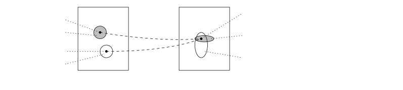
Figure 2: Two different points $g_{1},g_{2}$ in $G$ are mapped onto the same point in $P$. The elliptic ranges around the points illustrate the exploration kernels by suggesting the range of probable mutants. Thus, the two points $g_{1},g_{2}$ belong to one neutral set but represent two different exploration strategies.

What does this definition mean? Assume that one individual $g\in G$ is drifting in a neutral set $h^{-1}(x)$. Meanwhile, although its image $h(g)$ is not changing at all, the probability distribution of offsprings in $P$ (i.e. the exploration kernel $\tilde{M}_{g}$ associated to it) may change very well. This is how the definition captures the ability of exploration to adapt. See figure 2 for an illustration.

As a simple example we note that adding (neutral) mutation rate parameters aligns with this definition: Changing such strategy parameters actually is a neutral walk but varies the exploration kernels (e.g. by resizing them). Such and similar methods, may be understood as “local rescalings of neighborhood in $P$”; distances (probabilities to reach neighbors within one generation) are rescaled. However, such methods do not aim at varying the variational topology within $P$: the probabilities for mutations into the neighborhood change, the neighborhood itself though is not varied. The generality of our definition also captures the latter kind of variability and it will be a major goal of this paper to exemplify it by introducing neutral variations that do vary the variational topology on $P$.

In the following we will exclusively focus on self-adaptability of exploration as defined above.

Note:

Focusing only on self-adaptability (neglecting option (ii)), we want to emphasize that we always consider the GP-map $h$ to be fix, i.e. non-varying during evolution — and that this is not a restriction, not a loss of generality. If one would protest and claim that $h$ should be variable by depending on genes in $G$, we veto by stating that the formalism requires to collect all genetic parameters in the space $G$, that by definition the GP-map $h$ is the map which maps all $G$ on $P$, and thus it is formally incorrect to speak of $h$ as depending on genes in $G$.

Of course, others may have another point of view and this does not diminish the profound meaning of, e.g., Wagner and Altenberg’s statement that “the genotype-phenotype map is under genetic control and therefore evolvable.” [sec 2, par 9] — though from our point of view a questionable formulation.

4.1 Interpretations of neutrality

It is intuitive to believe that every little detail in nature fulfills “some purpose”; evolution would abandon all useless mechanisms and redundancies. The existence of something like neutrality in nature offends this intuition: A typical example is the fact that different codons are transcribed into the same amino acid, suggesting that certain nucleotide substitutions have no effect whatever on the phenotype or its fitness — they are neutral. Such issues initiated many investigations, pioneered by Motoo Kimura’s Neutral Theory [KimuraKimura1983]. In a later paper [KimuraKimura1986], he defends his theory against the selectionists’ criticism, who argued that neutral genes would be functionless, mere noise, and thus biologically implausible:

• “Sometimes, it is remarked that neutral alleles are by definition not relevant to adaptation, and therefore not biologically very important. I think that this is too short-sighted a view. Even if the so-called neutral alleles are selectively equivalent under a prevailing set of environmental conditions of a species, it is possible that some of them, when a new environmental condition is imposed, will become selected. Experiments suggesting this possibility have been reported by Dykhuizen & Hartl (1980) who called attention to the possibility that neutral alleles have a ‘latent potential for selection’. I concur with them and believe that ‘neutral mutations’ can be the raw material for adaptive evolution.” [kimura:86, page 345]

The last section gave a clear statement of how neutrality can be understood as “raw material for adaptive evolution”.

The interplay between neutrality and evolvability is a central topic also in other works. fontana:98, when investigating neutrality inherent in protein folding, claim that neutrality enables discontinuous transitions in the protein’s shape space (the space $P$): “[Transitions] can be triggered by a single point mutation only if the rest of the sequence [point in $G$] provides the appropriate context [neighborhood in $G$]; they are preceded by extended periods of neutral drift.” [last but one paragraph] Their arguments focus on the connectivity of neutral sets which can be analyzed theoretically by percolation theory. We agree on these generic ideas. A precondition is however that neutral sets exist and, most important, that exploration varies along these neutral sets — as we captured in the above definition.

A very intriguing study of such phenomena in nature is the one by stephens:99. They empirically analyze the codon bias and its effect in HIV sequences. Codon bias means that, although there exist several codons that code for the same amino acid (which form a neutral set), HIV sequences exhibit a preference of which codon is used to code for a specific amino acid. More precisely, at some places of the sequence codons are preferred that are “in the center of this neutral set” (with high neutral degree) and at other places codons are biased to be “on the edge of this neutral set” (with low neutral degree). It is clear that these two cases induce different exploration densities; the prior case means low mutability whereas the latter means high mutability. They go even further by giving an explanation for these two (marginal) exploration strategies: Loci with low mutability (trivially) cause “more resistance to the potentially destructive effect of mutation”, whereas loci with high mutability might induce a “change in a neutralization epitope which has come to be recognized by the immune system.” [introduction, par 4]

Finally, several models of landscapes with tunable neutrality have been proposed to theoretically investigate possible purposes of neutrality [BarnettBarnett2000, Newman and EngelhardtNewman and Engelhardt1998, Reidys and StadlerReidys and Stadler2001].

In this paper we present a simple setup to demonstrate the dynamics in neutral networks in appendix B. Using Eigen’s model we show a drift towards high neutral degree, i.e. towards representations of low mutability. This effect is important to understand the experiment we present in section 5.2.

5 Paradigms of self-adaptive exploration

The goal of this section is to exemplify the principles discussed above by simple and transparent (artificial) systems. In order to setup a running system we need to make some further decisions on

• (i) the problem (the space $P$),
  (ii) the GP-map (including the choice of $G$),
  (iii) the base density (population size, mutation rates on $G$, etc.),
  (iv) the evaluation (implementation of $E$),
  (v) the update rule $A$.

In the following $P$ will simply be strings over some alphabet ${\cal A}$; the problem is to minimize the (Hamming) distance to a given target string. Concerning point (iv) and (v), we will use rank-based selection, i.e. we evaluate proportionally to the rank of each individual and update the population by sampling this evaluation density. Point (ii) and (iii) need more thorough considerations:

A recursive, grammar-type GP-map.

We decide to implement the GP-map as a recursive mapping. More precisely, $h$ is representable as a composition of a single GP-generator $\hat{h}:\,G\to G$,

$$h=\underbrace{\hat{h}\circ..\circ\hat{h}}_{m(\cdot)\text{ times}}~{}:~{}G\to P\subset G~{}:~{}g\mapsto\underbrace{\hat{h}\circ..\circ\hat{h}}_{m(g)\text{ times}}(g)\;.$$ (13)

This inevitably requires a choice of $G$ such that $P\subset G$. The recursion depth $m$ may depend on the point $g\in G$. Generically, we require that each GP-generator affects (or entangles) only a few variables within $G$. The motivation is as follows: Structuredness of exploration, as discussed in section 3.1 and 3.2, means mutual information between variables that belong to the same phenotypic character and less mutual information else. We want the generator to represent elementary correlating effects (e.g. of interaction), i.e. to constitute elementary modules. For example, an elementary correlating effect is that one character depends also on another and a respective generator would introduce such mutual information by mapping one independent variable onto one which depends on other variables. An $NK$-reaction network is a basic example: the generator (the time step transformation) entangles $K$ variables to a new one.

Our examples will use a grammar-type recursive mapping. The space $G$ is organized as

$$G=P\times\big{[}{\cal A}\times P\big{]}^{r}\;,$$ (14)

which means that $g$ encompasses one structure $g_{0}\in P$ (called axiom) and $r$ tuples $g_{i}\in{\cal A}\times P$ (called rules). The GP-map $h$ applies to $g\in G$ by applying all rules to $g_{0}$; the symbols $l\in{\cal A}$ in each rule (actually the lhs label of a grammar rule) specify how to apply the rule. (The GP-generator is the single application of one rule to the axiom.) In our examples, the recursion depth $m$ is always fixed (so we need no terminal symbols or other complicated mechanisms.)

Such grammar-type encodings have been investigated in many other respects, e.g. by prusinkiewicz:89 and prusinkiewicz:90 discussing L-systems as natural representation of highly regular, plant-like structures; by kitano:90, gruau:95, lucas:95, and sendhoff:98 using grammar-encodings as representation of neural networks. However, these approaches are not based and motivated on a discussion of self-adaptive exploration. Thus, although in most cases the existence of neutral sets (equivalent representations) in grammar encodings is obvious, the importance to introduce (neutral) variations that explore these existing neutral sets and thereby explore different explorations strategies was not recognized and stressed. The next paragraph concerns the introduction of such variations.

Neutral variations in grammar-type encodings.

We turn to the choice of base density, i.e. variability on $G$. We assume that there exist canonical mutations on $P$, namely flip (with probability $\alpha$ per symbol), insertion, duplication and deletion (with probability $\gamma$ per string). Since $G$ is composed of structures of $P$ these mutations induce standard mutations on $G$.

However, to take all the considerations of section 4 into account, we additionally introduce neutral variations on $G$. These variations are supposed to allow for self-adaptability as defined above, i.e. they should allow neutral variations that vary exploration. In our examples we realize such variations by rule substitutions and creations. Specifically we introduce five kinds of variations of $g\in G$, which are likely to be neutral but need not always to be:

• (i) Pick one rule and one structure $\in P$ (any rhs or the axiom) within $g$; then apply the rule once to the structure.
  (ii) Pick one rule and one structure; check if the rhs of the rule is part of the structure; if so, replace this part by applying the rule inversely.
  (iii) Pick a structure and create a new rule by extracting a part out of the structure and replacing it by a symbol.
  (iv) Delete a rule if it is never applied during recursion.

All of these variations will occur with probability $\beta$ per rule (per structure in case (iii)).

5.1 Basic paradigm

Let $P$ be strings of the alphabet $\{0,1,x\}$. Consider the following two points $a,b\in G$ to represent the same point $0101$ in $P$:

$$a_{0}=01x\;,\quad a_{1}=(x\mapsto 01)\;,$$

$$b_{0}=xx\;,\quad b_{1}=(x\mapsto 01)\;.$$

If we assume that the rhs of $a_{1}$ and $b_{1}$ have considerable mutability, the exploration kernels of $a$ and $b$ are quite different: Probable (phenotypic) mutants of $a$ are $0111,0100,0110$, whereas $b$ is likely to produce mutants like $1111,0000,1010$. The difference of these two exploration densities is of topological nature.

In order to enable a transition between such different strategies, the exploration of the corresponding neutral set must be possible. In the upper example it is easy to define a neutral mutation from $a$ to $b$: The rule itself is to apply to the axiom. The inverse mutation requires an application of the rule from right to left, i.e., see if the rhs fits somewhere and substitute by the lhs. Our system incorporates these variations.

5.2 Two experiments: Variability of exploration and neutral drift

Let $P$ be the strings over the alphabet {a,b,c,d,e,f,g,h}. The function $f$ is the Hamming distance to the fixed target string abcdeabcdeabcdeabcdeabcde, i.e. 5 times abcde. To demonstrate a neutral drift we consider only one individual and initialize it with an axiom equal to the target and no rule. Selection is (1+1), i.e. at each time step one offspring is produced and selected if equally good or discarded if worse. As a result of neutral variations, the number of rules and the probability for regular mutations in the exploration density vary in correlation. This kind of variability of exploration is of topological nature. The point is, we gave an example where the topological characters of the exploration density vary over a connected neutral set. See figure 3.

We enhance this example by considering a population of 100 individuals and non-elitist, rank-based selection. All individuals are initialized as described above. The population drifts towards representations (points in the neutral set of the target string) with high neutrality. This effect is explained in detail in appendix B. Here, a high neutral degree coincides with representations of short description length (the sum of lengths of the axiom and rhs of rules). In order to achieve such compact representations, more rules are extracted and included in the representation. A visualization of the exploration density via mutual information maps exhibits its clear structure that corresponds to the target string’s structure. One may interpret that the system has “learned the problem’s structure”. See figure 4.

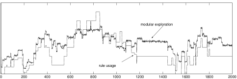
Figure 3: A single individual is tracked when drifting on a neutral set spanned by neutral substitutions in its grammar-encoding. Its exploration density is analyzed by taking 10 000 samples at each time step. ’Modular exploration’ counts the probability for mutations that occur equally at same positions in other blocks. These are blocks of 5 symbols as given by the target string: 5 $\times$ abcde. ’Rule usage’ counts how often rules are applied during recursion. [Population size $\mu=1$; mutation probabilities $\alpha=0.001$, $\beta=0.1$; recursion depth $m=10$; scaling of $y$-axes is only relative.]

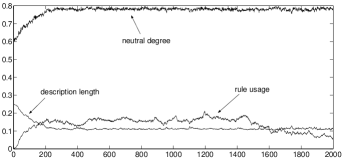
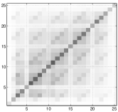
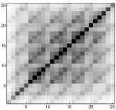
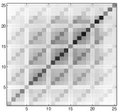
Figure 4: Upper plot: A population is tracked when drifting on a neutral set. Selection is non-elitist and rank-proportional and thus pushes the population towards higher neutral degree. This is achieved by finding representations of shorter description length of the modular target string (5 $\times$ abcde). (Description length equals the sum of the lengths of axiom and all rhs). This in turn is achieved by making use of rules. Lower plots: The mutual information between the 25 variables in the (phenotypic) exploration density is displayed as a matrix. The three plots correspond to times 50, 500, and 2000. The regular, 5-modular structure of exploration is clearly visible. [Population size $\mu=100$; mutation probabilities $\alpha=\beta=0.02$; target: 5 $\times$ abcde; recursion depth $m=3$; scaling of $y$-axes is exact for neutrality, only relative for the rest; scaling of gray-shading is only relative.]

6 Conclusions

Major parts of this paper are concerned to develop an integrated language for evolutionary search based on the formalism of stochastic search and emphasizing the exploration density and its parameterization. The benefit is a unified view on different specific approaches, their commonness and differences. For example, at first sight it is hard to see what a CMA evolutionary strategy has in common with the codon bias in HIV sequences. The answer is: both of them are concerned to model the variability of future offsprings, the exploration density; both of them by using a kind of genotype-phenotype mapping (an affine transformation in the first case). Also notions such as pleiotropy and functional phenotypic complex can properly be defined on the basis of this language. This allows to make contact between biological and computational research. The functional meaning of a genotype-phenotype mapping is illuminated by interpreting it as a lift of an exploration density and topology on the search space. We showed that a non-injective genotype-phenotype mapping can lift different exploration strategies, different topologies to the same phenotype. This is the core of how we define self-adaptability of exploration. The definition overcomes the formal weakness of previous definitions and is as general as the language it is based on. The definition opens a completely new view on the meaning of neutrality.

In the experimental part of this paper we presented elementary examples of these concepts. We illustrated the structure of exploration by a gray-shade map of the mutual information within the exploration density, a gray-shade map of pleiotropy. We exemplified its variability during neutral drifts. And we demonstrated successful self-adaptability of exploration where in the end the structure of exploration perfectly matches the structure of the problem.

We will now discuss some further implications of the new view we have developed in this paper:

(i) On modularity, structuredness, and evolvability.

Given a system that functions well, how should one define what a module or a functional complex is? One only observes that all parts together work well as a whole. A common idea is that modules are characterized by high interactivity within them. By high interactivity we mean that there are high correlations between units during the time of functioning. These are completely different kinds of correlations than correlations between units in the evolutionary variability. It is though possible to draw a link: Having units that are highly interacting during functioning, the fitness might strongly depend on their teamwork. If this is the case, also the evaluation density should incorporate high correlations between the units (i.e. the units form a functional phenotypic complex). Now, if the exploration density should approximate the evaluation density, we also find these correlations in the evolutionary variability.

Thus, when talking about modules, one should be aware of the interrelations between these three levels of correlations: (1) during functioning, (2) in the evaluation density, (3) in the exploration density. Our definition of a functional phenotypic complex refers to the 2nd level – the evaluation density. Our hypothesis is that the advantage of structured systems (and thus the selective pressure towards structure) stems from the 3rd level:

• Systems are structured, not because this is the only possible way of functioning, but because it is advantageous for variability. The advantage of structured variability is its capability to explore by approximating the “problem’s structure”, the structure of the evaluation density.

This capability should be called evolvability.

For example, parts of a system that contribute separately to fitness should be varied and optimized in parallel without potentially disturbing correlations; whereas parts of a system that only contribute to fitness when they are tuned on each other should be varied in correlation in order to preserve this tuning.

(ii) On redundancy and neutrality

Neutrality is often thought of as redundancy. From our point of view, this is very misleading. As we pointed out in the context of self-adaptability, although all the genotypes in a neutral set encode the same phenotype, they may have very different exploration kernels. Thus, such genotypes may carry different information. One cannot speak of redundancy if different and relevant information is encoded. If, however, genotypes in a neutral set have identical exploration kernels (in the genotype space), then they are indeed redundant. Redundancy is necessarily neutral, but neutrality is not necessarily redundant.

(iii) On compact representations

Assume we use a Bayesian network to model the structure of exploration. Then we will explicitly encode the correlations between all phenotypic variables. In contrast, our second example shows how compact representations correspond to highly structured exploration and can be found by using recursive codings. The idea is that each recursion introduces correlations in the variables. The neutral drift towards high neutral degree (see appendix B) induces a selective pressure towards short representations.

(iv) On grammar-type encodings

In grammar-type encodings, some single genotypic variables (genes) might effectively represent whole groups of phenotypic variables. Thus, when we model dependencies between variables, we can also model dependencies between whole groups of phenotypic variables and not only between single phenotypic variables as in the direct modeling ansatz. This allows to introduce deep hierarchical dependencies in the exploration density.

Most existing approaches to grammar encoding are motivated by the fact that grammars can represent regular structures with short description length. Instead, we claim that the most interesting point about grammars is their capability to introduce structure in the variability, as demonstrated in our examples. In order to explore these capabilities in a self-adaptive manner, the inclusion of neutral variations in recursive or grammar-type encodings is of crucial importance. This point seems neglected in the literature.

We rigorously support Kimura’s “belief that ‘neutral mutations’ can be the raw material for adaptive evolution” [KimuraKimura1986].

Appendix A The exploration model of different state-of-the-art evolutionary algorithms

To stress the importance of the concept of exploration modeling we want to show that the main difference between specific evolutionary algorithms is their ansatz to model exploration. In order to do so, we embed specific algorithms in our formalism. In particular we chose to analyze the CMA algorithm and three recent approaches which belong to the class of “probabilistic model-building genetic algorithms” (PMBGAs), see [Pelikan, Goldberg, and LoboPelikan et al.1999]. All of these realize adaptive (but not self-adaptive) exploration.

Covariance Matrix Adaptation (CMA),

[Hansen and OstermaierHansen and Ostermaier2000]. The search space is continuous, $P=\mathbb{R}^{n}$. The CMA algorithm maintains as parameters $q$ only one (center of mass) point $p\in P$, the symmetric covariance matrix $C$, and some adaption rate parameters. The exploration density $M_{q}$ is given by a linear transformation (via $C$) of a Gaussian distribution around $p$. In practise, the algorithm generates $\lambda$ normally distributed mutation vectors $z_{i}\in\mathbb{R}^{n}$, transforms all of these vectors by multiplying the matrix $C$, and adds these vectors to the center of mass $p$ in order to generate the new $\lambda$ samples. After evaluation of the samples it is updated as follows: $p$ is moved to the center of mass of the selected samples and $C$ is adapted as

$$C^{(t+1)}=(1-c)\;C^{(t)}+c\;z\otimes z\;.$$ (15)

Here, $c$ is some adaption constant and $z$ is the average of the selected mutations vectors. (hansen:00, Eq. 15, write $z(z)^{T}$ instead of $z\otimes z$). The point is that $z\otimes z$ is the unique symmetric matrix which maps the equally distributed vector $y=(\frac{1}{n},..,\frac{1}{n})$ to $z$. Thus, the update rule for $C$ corresponds to our generic approaching update whereas $p$ adopts the new center of mass.

Dependency tree modeling,

[Baluja and DaviesBaluja and Davies1997]. Here, the search space is discrete, $P=X^{n}$. In their algorithm, the parameter $q$ that describes the next exploration density is a dependency tree. Thus, the model is restricted to encode only pair-wise dependencies between variables. At each time step, $\lambda$ samples are generated from this exploration density; the samples are evaluated and the best $\mu$ of them are selected. A probability density $A$ of previously selected points is adapted by including those newly selected ones (generically $A\leftarrow(1-\alpha)\,A+\alpha\,[E_{s^{(t)}}]_{\mu}$). Then the dependency tree is updated by minimizing the Kullback-Leibler divergence between $A$ and $M_{q}$. The tree’s update is an adopting since it approximates $A$, whereas $A$ itself is updated according to an approaching update.

Factorized Distribution Algorithm (FDA),

[Mühlenbein, Mahnig, and RodriguezMühlenbein et al.1999]. Again, $P=X^{n}$ is discrete. The parameters $q$ describe the conditional dependencies in pairs, triples, quadruples, etc. of variables. (To be exact, the algorithm comprises also some elitists.) The model is quite general but it relies on pre-fixed knowledge on which pairs, triples, etc. exactly are to be parameterized. At each time step, the dependencies within the distribution of evaluated and selected points are calculated and assigned to $q$. Therefore, this is an adopting update.

Bayesian Optimization Algorithm (BOA),

[Pelikan, Goldberg, and Cantú-PazPelikan et al.2000]. $P=X^{n}$ is discrete. Here, $q$ is a general Bayesian dependency network that explicitly encodes the exploration density. Thus, the model is not limited in representing arbitrary orders of correlation and it is flexible in which variables are dependent by inserting and deleting connections in the network. After selection, the network is recalculated in order to minimize (e.g. with a greedy algorithm) the distance (e.g. with respect to the Bayesian Dirichlet Metric) between $M_{q}$ and the distribution of selected. This is, except for elitists, also an adopting update.

Appendix B Illustrating neutral dynamics

As an illustration of neutral dynamics we present a simple example. We assume that the search space $P$ is discrete and rather small, $|P|=\lambda$. $\Lambda$ denotes the space of densities over $P$, which actually is a simplex. Parameter $q\in Q$ is such a density, $Q=\Lambda$, and the exploration density $M_{q}$ is a mutation $\tau\,q\in\Lambda$ of this density. This example omits sampling and thus evaluation $E:\,\Lambda\to\Lambda$ directly applies to $M_{q}=\tau\,q$. The update rule is the adopting:

$$q^{(t+1)}=E\,\tau\,q^{(t)}\;,\quad q^{(t+1)}_{i}=\sum_{j,k=1}^{\lambda}E_{ij}\,\tau_{jk}\,q^{(t)}_{k}\;,\quad$$ (16)

whereby we actually formulated Eigen’s model (see e.g. [Eigen, McCaskill, and SchusterEigen et al.1989]) in our notation. Finding the eigenvectors of $E\,\tau$ means finding a stationary population density. Their eigenvalues describe their growth factor and the eigenvector with highest eigenvalue will describe the final attractor — the quasi-species. In the presence of a neutral set $N$ (here a set of indices) we assume that only individuals on this neutral set are evaluated positively and without co-evolutionary (interacting) effects, i.e., $E$ is diagonal and

$$E:\,\Lambda\to\Lambda\;,\quad p_{i}\mapsto\sum_{j}E_{ij}\,p_{j}=E_{ii}\,p_{i}=\left\{{0\atop e_{i}(p)\,p_{i}}\quad{i\not\in N\atop i\in N}\right.\quad.$$ (17)

neutral set $N\subset P$:

First experiment

density $q\in\Lambda$:

mutated density $\tau\,q\in\Lambda$:

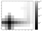
Second experiment

density $q\in\Lambda$:

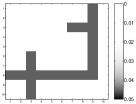
mutated density $\tau\,q\in\Lambda$:

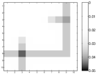
Figure 5: The search space $P$ is represented as a 10$\times$10 board. The neutral set is embedded as depicted on the left. The exploration matrix $\tau$ corresponds to a mutation rate of $0.1$ in each of the four directions (up,down,right,left). In the first experiment, when evaluation is straightforward, e.g. fitness-proportional, it is impressive to see how strong the attraction towards the crossing with neutral degree $1$ (with four neutral neighbors) is. In the second experiment, where evaluation enforces a kind of local conservation of population density, the population is equally distributed on the neutral set, but exploration on places with high neutral degree is proportionally higher because they have more neighbors from which they “receive” offsprings.

We investigate two options for the evaluation factor $e_{i}(p)$. The first and straightforward option is that all positions on the neutral set are evaluated equally, then

$$e^{1}_{i}(p)=\frac{1}{\sum_{j\in N}p_{j}}$$ (18)

is just the appropriate normalization factor. This option is realized e.g. for fitness-proportional evaluation (when fitness on $P\setminus N$ vanishes) but also for fair ranking. For the second option we enforce such positions on the neutral set with low neutral degree — inverse-proportionally to the neutral degree:

$$e^{2}_{i}(p)=\frac{1/d_{i}}{\sum_{j\in N}(p_{j}/d_{j})}\;,\quad d_{i}:=\sum_{k\in N}\tau_{ik}\;.$$ (19)

The quantity $d_{i}$ is the probability for an offspring of individual $i$ to be an element of $N$. Thus, this option increases the evaluation of $i$ such that the probability to provide an offspring in $N$ becomes equal for all $i\in N$. This can be compared to a local conservation of population density: Effectively, each parent in $N$ will with equal probability contribute a viable offspring to the next generation. Such a type of selection can be realized by local selection mechanisms: From each parent produce many offsprings, let only the best of these offsprings compete with others. As a result, the quasi-species is simply constant on $N$ and vanishes elsewhere, $q_{i\in N}=1/|N|$, $q_{i\not\in N}=0$:

$$p_{i}=(\tau\,q)_{i}=\sum_{j\in N}\tau_{ij}\,q_{j}=\frac{d_{i}}{|N|}\;,$$ (20)

$$(E\,\tau\,q)_{i\in N}=\frac{1/d_{i}}{\sum_{j\in N}(p_{j}/d_{j})}\;p_{i}=\frac{1}{|N|}=q_{i}\;.$$ (21)

The mutated density $p_{i}$ is proportional to $d_{i}$ (which, for individuals out of $N$, does not denote the neutral degree but rather the probability for offsprings in $N$). Diversity is much higher than for the first type of evaluation. See figure 5.

The first experiment is an explanation for the dynamics we observe in section 5.2. We included the second experiment because it realizes what one might intuitively have expected: on a neutral set the population is distributed equally and with high diversity. We showed what kind of evaluation one has to choose to fulfill this expectation.

The findings are conform with Nimwegen’s nimwegen:99 little examples of random or selective walks on a neutral set: A blind ant would try one (random) neighboring genotype and walk to it if it has same fitness or stay otherwise. A myopic ant would find all neighbors with same fitness and walk to one (random) of those. He finds that, in temporal average, the blind ant stays equal times at each genotype of the neutral set whereas the myopic ant stays longer at centers of the neutral set (i.e. $\propto$ the neutral degree). The myopic ant, since it always finds a neutral neighbor, corresponds to our second example.

References

- [\citeauthoryearBaluja and DaviesBaluja and Davies1997] Baluja, S. and S. Davies (1997). Using optimal dependency-trees for combinatorial optimization: Learning the structure of the search space. In Proceedings of the Fourteenth International Conference on Machine Learning (ICML-97), pp. 30–38.
- [\citeauthoryearBarnettBarnett2000] Barnett, L. (2000). Ruggedness and neutrality - the NKp family of fitness landscapes. In Sixth International Conference on Artificial Life (ALIVE-VI), pp. 18–27.
- [\citeauthoryearEiben, Hinterding, and MichalewiczEiben et al.1999] Eiben, A. E., R. Hinterding, and Z. Michalewicz (1999). Parameter control in evolutionary algorithms. IEEE Transactions on Evolutionary Computation 3, 124–141.
- [\citeauthoryearEigen, McCaskill, and SchusterEigen et al.1989] Eigen, M., J. McCaskill, and P. Schuster (1989). The molecular quasispecies. Advances in chemical physics 75, 149–263.
- [\citeauthoryearFontana and SchusterFontana and Schuster1998] Fontana, W. and P. Schuster (1998). Continuity in evolution: On the nature of transitions. Sience 280, 1431–1433.
- [\citeauthoryearGruauGruau1995] Gruau, F. (1995). Automatic definition of modular neural networks. Adaptive Behaviour 3, 151–183.
- [\citeauthoryearHansen and OstermaierHansen and Ostermaier2000] Hansen, N. and A. Ostermaier (2000). Completely derandomized self-adaption in evolutionary strategies. Evolutionary Computation, special issue on self–adaptation, to appear.
- [\citeauthoryearKimuraKimura1983] Kimura, M. (1983). The Neutral Theory of Molecular Evolution. Cambridge University Press.
- [\citeauthoryearKimuraKimura1986] Kimura, M. (1986). DNA and the Neutral Theory. Philosophical Transactions, Royal Society of London B312, 343–354.
- [\citeauthoryearKitanoKitano1990] Kitano, H. (1990). Designing neural networks using genetic algorithms with graph generation systems. Comples Systems 4, 461–476.
- [\citeauthoryearLucasLucas1995] Lucas, S. (1995). Growing adaptive neural networks with graph grammars. In Proceedings of European Symposium on Artificial Neural Networks (ESANN ’95), pp. 235–240.
- [\citeauthoryearMühlenbein, Mahnig, and RodriguezMühlenbein et al.1999] Mühlenbein, H., T. Mahnig, and A. O. Rodriguez (1999). Schemata, distributions and graphical models in evolutionary optimization. Journal of Heuristics 5, 215–247.
- [\citeauthoryearNewman and EngelhardtNewman and Engelhardt1998] Newman, M. and R. Engelhardt (1998). Effects of neutral selection on the evolution of molecular species. Proc. R. Soc. London B265, 1333–1338. Los Alamos e-Print adap-org/9712005.
- [\citeauthoryearPelikan, Goldberg, and Cantú-PazPelikan et al.2000] Pelikan, M., D. E. Goldberg, and E. Cantú-Paz (2000). Linkage problem, distribution estimation, and bayesian networks. Evolutionary Computation 9, 311–340.
- [\citeauthoryearPelikan, Goldberg, and LoboPelikan et al.1999] Pelikan, M., D. E. Goldberg, and F. Lobo (1999). A survey of optimization by building and using probabilistic models. IlliGAL Report 99018.
- [\citeauthoryearPrusinkiewicz and HananPrusinkiewicz and Hanan1989] Prusinkiewicz, P. and J. Hanan (1989). Lindenmayer Systems, Fractals, and Plants, Volume 79 of Lecture Notes in Biomathematics. Springer, New York.
- [\citeauthoryearPrusinkiewicz and LindenmayerPrusinkiewicz and Lindenmayer1990] Prusinkiewicz, P. and A. Lindenmayer (1990). The Algorithmic Beauty of Plants. Springer, New York.
- [\citeauthoryearReidys and StadlerReidys and Stadler2001] Reidys, C. M. and P. F. Stadler (2001). Neutrality in fitness landscapes. Applied Mathematics and Computation 117, 321–350. Santa Fe Institute preprint 98-10-089.
- [\citeauthoryearSchusterSchuster1996] Schuster, P. (1996). Landscapes and molecular evolution. Physica D 107, 331–363.
- [\citeauthoryearSendhoff and KreutzSendhoff and Kreutz1998] Sendhoff, B. and M. Kreutz (1998). Evolutionary optimization of the structure of neural networks using recursive mapping as encoding. In Artificial Neural Nets and Genetic Algorithms – Proceedins of the 1997 International Conference, pp. 370–374.
- [\citeauthoryearSmith and FogartySmith and Fogarty1997] Smith, J. and T. Fogarty (1997). Operator and parameter adaption in genetic algorithms. Soft Computing 1, 81–87.
- [\citeauthoryearStephens and WaelbroeckStephens and Waelbroeck1999] Stephens, C. and H. Waelbroeck (1999). Codon bias and mutability in HIV sequences. Molecular Evolution 48, 390–397.
- [\citeauthoryearvan Nimwegen and Crutchfieldvan Nimwegen and Crutchfield1999] van Nimwegen, E. and J. P. Crutchfield (1999). Neutral evolution of mutational robustness. Santa Fe Working Paper 99-07-041.
- [\citeauthoryearVoseVose1999] Vose, M. D. (1999). The Simple Genetic Algorithm. MIT Press, Cambridge.
- [\citeauthoryearWagner and AltenbergWagner and Altenberg1996] Wagner, G. P. and L. Altenberg (1996). Complex adaptations and the evolution of evolvability. Evolution 50, 967–976.
- [\citeauthoryearZhigljavskyZhigljavsky1991] Zhigljavsky, A. A. (1991). Theory of global random search. Kluwer Academic Publishers.