Deconvolution problems in x-ray absorption fine structure

Abstract

A Bayesian method application to the deconvolution of EXAFS spectra is considered. It is shown that for purposes of EXAFS spectroscopy, from the infinitely large number of Bayesian solutions it is possible to determine an optimal range of solutions, any one from which is appropriate. Since this removes the requirement for the uniqueness of solution, it becomes possible to exclude the instrumental broadening and the lifetime broadening from EXAFS spectra. In addition, we propose several approaches to the determination of optimal Bayesian regularization parameter. The Bayesian deconvolution is compared with the deconvolution which uses the Fourier transform and optimal Wiener filtering. It is shown that XPS spectra could be in principle used for extraction of a one-electron absorptance. The amplitude correction factors obtained after deconvolution are considered and discussed.

I Introduction

The chief task of the extended x-ray absorption fine-structure (EXAFS) spectroscopy, determination of interatomic distances, rms fluctuations in bond lengths etc., is solved mainly by means of the fitting of parameterized theoretical curves to experimental ones. However, there exist obstacles for such a direct comparison: theory limitations and systematic errors. Among latter are various broadening effects. Fist of all, (i) this is the broadening arising from the finite energy selectivity of monochromator and the finite angular size of the x-ray beam. (ii) The absorption even of strictly monochromatic x-ray irradiation by the electrons of a deep atomic level gives rise to photoelectrons with the finite energy dispersion due to the finite natural width of this level and the finite lifetime of the core-hole. (iii) For x-ray energies far above the absorption edge the process of photoelectron creation (the outgoing from an absorbing atom) and the process of its propagation occur for essentially different time intervals. In other words, just created, the photoelectron ‘does not know’ where and how it will decay. Therefore the photoionization from the chosen atomic level and excitation of the remaining system can be considered as independent processes, and hence the total absorption cross-section, as a probability density of two independent random processes, is given by the convolution of a one-electron cross-section and excitation spectrum $W(\Delta E)$. The latter is the probability density of the energy $\Delta E$ capture at the electron-hole pair creation and is the quantity measured in x-ray photoemission spectroscopy (XPS). For light elements there are examples of such deep and lengthy enough XPS spectra (see figure 1, taken from [1]).

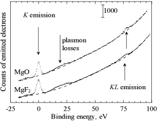
FIG. 1.: From [1]: XPS spectra of MgO and MgF₂ in the vicinity of the Mg 1$s$ peak. Two secondary structures, due to plasmon losses and to double-electrton $KL_{2,3}$ excitations, are detected. Zero of energy is placed at Mg $K$ level ($\sim 1300$ eV).

For all three cases the measured absorption coefficient $\mu_{\rm m}$ is given by the convolution:

$$\mu_{\rm m}(E)=W*\mu\equiv\int W(E-E^{\prime})\mu(E^{\prime})\,{\rm d}E^{\prime},$$ (1)

where the broadening profile $W(\Delta E)$ and the meaning of the function $\mu$ depend on the considered problem. These can be, correspondingly: x-ray spectral density after the monochromator and the cross-section of ideally monochromatic irradiation; the Lorentzian function and the cross-section with a stationary initial level (of zero width); the excitation spectrum and a one-electron cross-section.

It is the common practice in modern EXAFS spectroscopy to account for the broadening processes (i)–(iii) at the stage of theoretical calculations by introducing into the one-electron scattering potential the imaginary correlation part which represents the average interaction between photoelectron and hole and their own polarization cloud; in doing so, the choice of the correlation part is dictated by empiric considerations and can be different for different systems.

Another approach to the account for the broadening processes is to solve the integral equation (1) for the unknown $\mu$. To find some solution of this equation is quite not difficult to do, the simplest way is to use the theorem about the Fourier transform (FT) of convolution. However, it is known that the problem of deconvolution is an ill-posed one: it has an unstable solution or, in other words, the infinitely large number of solutions specified by different realizations of the noise. Thus, there is evident necessity for determination of an optimal, in some sense, solution. Yet a less evident approach exists: to find an appropriate functional of the solution which itself be stable.

A number of works have been addressed the problem of deconvolution, among them those concerning the x-ray absorption spectra. Loeffen et al. [2] applied deconvolution with the Lorentzian function partly eliminating the core-hole life-time broadening. They used fast FT and the Wiener filter which is determined from the noise level which, in turn, is specified by the choice of the limiting FT frequency above which the signal is supposed to be less than noise. The arbitrariness of such a choice gives rise to rather different deconvolved spectra, which although remained obscured in [2].

Recently, for the deconvolution problem with a Lorentzian function Filipponi [3] used the FT and proposed the idea of the decomposition of an experimental spectrum into the sum of linear contribution, a special analytic function representing the edge and oscillating part. For the Lorentzian response, the deconvolution for the first two contribution is found analytically, for the latter one, numerically. The advance of such a decomposition is in that fact that now the FT of the oscillating part is not dominated by the very strong signal of low frequency, therefore the combination of forward and backward FT gives less numerical errors. Notice that this method is solely suitable for the analytically given response. In addition, in [3] the choice of the filter function (Gaussian curve) and its parameterization remained vague. Therefore the issue on the uniqueness or optimality of the found solution was left open.

In early work [4], for the solution of ill-posed problems the statistical approach was proposed. Following that work, in the present paper we shall consider the deconvolution problem in the framework of Bayesian method, detailed formalism of which was described in [5]. Since the parameterization is naturally involved in the Bayesian method, there exists a principle possibility to choose an optimal, in some sense, parameter. Here we shall scrutinize the problem of such a choice which is relevant to any spectroscopy. We shall show that this problem is absent in EXAFS spectroscopy because though the EXAFS spectrum itself does depend on the regularization parameter, its FT does not in the range of real space used for the analysis. In Sec. II we discuss the choice of the optimal deconvolution for a model Gaussian response and compare the results of Bayesian approach with the results of FT combined with Wiener filtering. In Sec. III we utilize the deconvolution to an experimental spectrum in order to eliminate the aforementioned broadening processes.

II The choice of optimal deconvolution

First of all, we shall show that the deconvolution problem really has the infinitely large number of solutions. In the present paper we use for examples the absorption spectrum of Nd_1.85Ce_0.15CuO_4-δ above Cu $K$ edge collected at 8 K in transmission mode at LURE (beamline D-21) using Si(111) monochromator and harmonics rejecting mirror; energy step $\sim 2$ eV, total amount of points 826 (from 8850 eV to 10500 eV), each one recorded with integration time of 10 s. Let us take for a while for the response function a simple model form: $W(E)=C\exp(-E^{2}/2\Gamma^{2})$, where $C$ normalizes $W$ to unity, $\Gamma$ is chosen to be equal to 4 eV.

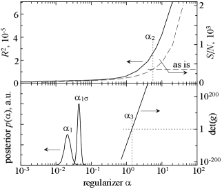
FIG. 2.: The quality of the deconvolution $R^{2}$ vs. regularization parameter $\alpha$ (solid). Dashed lines — signal-to-noise ratio before and after deconvolution. Two peaks — the posterior density functions $p(\alpha|\bf{d})$ (left) and $p(\alpha|\bf{d},\sigma)$ (right) for the regularization parameter $\alpha$. Straight line — the determinant of Bayesian matrix as a function of $\alpha$.

In [5] we showed how to construct a regularized solution of the convolution equation in the framework of the Bayesian approach. For that, one needs to find eigenvalues and eigenvectors of a special symmetric $N\times N$ matrix determined by the experimental spectrum, $N$ is the number of experimental points. Using that approach, find a solution $\mu(E)$ for an arbitrary regularization parameter $\alpha$ and perform its convolution with $W$. The $\hat{\mu}_{\rm m}$ obtained, ideally, must coincide with $\mu_{\rm m}$. Introduce the characteristics of the solution quality, the normalized difference of these curves:

$$R^{2}=\sum_{i}(\mu_{{\rm m}i}-\hat{\mu}_{{\rm m}i})^{2}\Bigr{/}\sum_{i}\mu_{{\rm m}i}^{2},$$ (2)

where the summation is done over all experimental points. Figure 2 shows the dependence $R^{2}$ on $\alpha$. That fact that the quality of the found solutions is practically the same for all $\alpha\lesssim 1$ is a clear manifestation of ill-posedness of the problem: there is no a unique solution. How to chose an optimal one? It turns out, that for purposes of EXAFS spectroscopy there is no need of that and any solution from the optimal range (here, $\alpha\lesssim 1$) is suitable. At arbitrary $\alpha$ from the optimal range found the deconvolution $\mu(E)$, extract the EXAFS function $\chi(k)\cdot k^{w}$ in a conventional way, where $k$ is the photoelectron wave number, and find its FT. In figure 3 we show the EXAFS-functions obtained after the Bayesian deconvolution with $\alpha=1$ and $\alpha=0.01$, and their FT’s. As seen, although the EXAFS-function itself does depend on $\alpha$, its FT practically does not. Thus, if one uses for fitting a range of $r$-space (in our example, up to $r_{\rm max}=8\,$Å) or filtered $k$-space, the problem of search for the optimal $\alpha$ is not relevant. Nevertheless, below we propose several approaches to the solution of this problem, for instance for XANES spectroscopy needs.

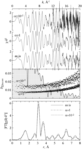
FIG. 3.: $\chi\cdot k^{2}$ obtained without deconvolution and after that with $\alpha=1$ and $\alpha=0.01$. In the middle — the envelope of the initial $\chi$ and rms deviations of the deconvolved values (dots). Below — the absolute values of the Fourier transform (the dashed and the dotted curves practically merge).

(1) For the regularization parameter $\alpha$ itself one can introduce the posterior probability density function [4, 5] and choose $\alpha$ with a maximum probability density. It can be done either using the most probable value of noise or assuming the standard deviation $\sigma$ of the noise of the absorption coefficient to be known (for our spectrum $\sigma=9\cdot 10^{-4}$, as determined from the FT following [6]). In figure 2 these probability densities are drawn as, correspondingly, $p(\alpha|\bf{d})$ and $p(\alpha|\bf{d},\sigma)$, and their most probable values are $\alpha_{1}=0.021$ and $\alpha_{1\sigma}=0.044$.

(2) The optimal regularization can be determined from the consideration of the signal-to-noise ratio $S/N$. The Shannon-Hartley theorem states that $I_{\rm max}=B\ln{(1+S/N)}$, where $I_{\rm max}$ is the maximum information rate, $B$ is the bandwidth. The authors of [2] are of opinion that deconvolution is a mathematical operation that conserves information. Therefore from the theorem follows that one pays for an increase in bandwidth, resulted from deconvolution, via a reduction in $S/N$ ratio. The thesis on $I_{\rm max}$ conservation is quite questionable, since for deconvolution one should introduce additional independent information about the profile of broadening. What quantity is conserved in deconvolution is hard to tell. Here to the contrary, for the optimal $\alpha$ we demand to conserve $S/N$. Define $S/N$ as the ratio of mean values of the EXAFS power spectrum over two regions, $r<15$ Å and $15<r<25$ Å. The regularization parameter at which the $S/N$ is conserved is denoted in figure 2 as $\alpha_{2}=5.54$. The signal-to-noise ratio can be defined in a different way. Since the Bayesian methods work in terms of posterior density functions, for each experimental point one can find not only the mean deconvolved value but also the standard deviation $\delta\mu_{\rm deconv}$ from which one finds $\delta\chi=\delta\mu_{\rm deconv}/\mu_{0}$, where $\mu_{0}$ is the atomic-like absorption coefficient constructed at the stage of EXAFS function extraction. It is reasonable to compare $\delta\chi$ values with the envelope of EXAFS spectrum (figure 3, middle). As seen, at small $\alpha$ the noise dominates over the signal in the extended part of the spectrum. The regularization parameter at which they match is the optimal one, $\alpha_{2}$.

(3) For the Bayesian deconvolution it is necessary to find eigenvalues and eigenvectors of a special symmetric matrix $g$. It turns out that the determinant of this matrix varies with $\alpha$ over hundreds orders of magnitude. At small $\alpha$’s the matrix is poorly defined, large $\alpha$’s yield very large $\det(g)$ (figure 2). Both cases give large numerical errors because of ratios of very small or very large values in calculations. As an optimal parameter we choose $\alpha_{3}=1.41$ at which $\det(g)\sim 1$.

The cases (1) and (2) require to determine the noise level, which demands additional variables (for instance, the limiting frequencies of FT). The case (3) does not explicitly concern the noise. Due to the dependence of $\lg[\det(g)]$ on $\alpha$ appears to be linear, which readily allows one to find the optimal parameter, the case (3) is more preferable from the practical point of view. Below, for deconvolution of the real broadening processes we use the optimal parameter $\alpha_{3}$.

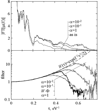
FIG. 4.: Module of the FT of initial $\mu_{\rm m}$ and deconvolved $\mu$ at different $\alpha$. Below — filters transforming $\mu_{\rm m}(\tau)$ to $\mu(\tau)$ obtained after Bayesian deconvolution (thin solid lines), after deconvolution based on the FT (dashed line), and after deconvolution based on the combination of the FT and Wiener filtering (thick solid line).

It is of certain interest to compare the Bayesian method of deconvolution with the widely known method combining optimal Wiener filtering and the convolution theorem, where the conjugate variables of the FT are not $k$ and $2r$ adopted in EXAFS but $E$ and $\tau$. According to the theorem, $\mu_{\rm m}(\tau)=W(\tau)\cdot\mu(\tau)$, where for our model Gaussian response $W(\tau)=\exp(\Gamma^{2}\tau^{2}/2)$. A simple back FT of the ratio $\mu_{\rm m}(\tau)/W(\tau)$ will give the thought solution $\mu(E)$ but very noisy. Therefore $\mu_{\rm m}(\tau)$ at large $\tau$ has to be smoothed. Figure 4 shows module of the FT of the measured spectrum and of the Bayesian deconvolved spectra. The latter are merged at $\tau\lesssim 0.25$ eV^-1. In the bottom part of the figure the ratios $|{\rm FT}\mu_{\rm deconv}|/|{\rm FT}\mu_{\rm m}|$ are shown for different $\alpha$. As seen, the Bayesian deconvolution performs the effective filtration of spectra with the limiting frequency $\tau_{\rm max}$ depending on $\alpha$.

The optimal, in the least-square sense, Wiener filter is expressed as [7]: $\Phi(\tau)=(1+|n(\tau)|^{2}/|{\rm FT}\mu_{\rm m}|^{2})^{-1}$, where $|n(\tau)|^{2}$ is the power spectrum of the noise replaced here by 0.01, the mean value of $|\mu(\tau)|^{2}$ over the range $\tau>0.4$ eV^-1. As seen in figure 4, the effective Wiener filter $W(\tau)\Phi$ transforming $\mu_{\rm m}(\tau)$ to $\mu(\tau)$ is close to the effective filter of the Bayesian deconvolution with $\alpha=1\approx\alpha_{3}$. Notice, however, that the limiting frequency for the estimation of noise power spectrum was chosen rather arbitrarily.

In closing this section, it should be noticed that apart from the possibility of determination of the deconvolution errors and the possibility of the optimal regularization parameter choice, the Bayesian deconvolution has the advantage of the capability to take into account a priori information about the smoothness and shape of the solution (see details in [5]). In addition, in the Bayesian method the response function $W(E-E^{\prime})$ could be of more general form $W(E-E^{\prime},E)$, which will be useful for deconvolution of the instrumental broadening because monochromator energy resolution depends noticeably on the angular position and, hence, on the energy of the output x-ray beam.

III Applications of deconvolution

We have seen that the Bayesian method proves to be effective for deconvolution of EXAFS spectra, and the choice of the regularization parameter appears to be irrelevant. Now we perform the deconvolution of various types of broadening, for which purpose specify the corresponding response functions $W(E-E^{\prime},E)$.

A Instrumental broadening

The monochromator resolution is determined by the rocking curve width $\delta\theta_{B}$ and by the vertical beam divergence $\delta\theta_{\perp}$. For the monochromator Si(111) at $E=9$ keV the rocking curve width is $\delta\theta_{B}=32.4$ $\mu$rad (FWHM) [8], the beam divergence (LURE, D-21) $\delta\theta_{\perp}=150$ $\mu$rad. Strictly speaking, the resulting spectral distribution is given by the convolution of rocking curve and the angular beam profile. But since $\delta\theta_{B}\ll\delta\theta_{\perp}$, the energy selectivity is determined by $\delta\theta_{\perp}$, namely: $\delta E_{\perp}/E=\delta\theta_{\perp}\cot\theta_{B}=\delta\theta_{\perp}\sqrt{(2Ed/ch)^{2}-1}$, where $\theta_{B}$ is Bragg angle, $d$ is Bragg plane spacing. Modelling the spectral distribution by a Gaussian function, one obtains:

$\displaystyle W(E-E^{\prime},E)\propto\exp\left[-\frac{(E-E^{\prime})^{2}}{2\sigma^{2}_{\perp}(E)}\right],\sigma_{\perp}(E)=\frac{\delta E_{\perp}(E)}{2\sqrt{2\ln 2}},$

where the normalization constant must be calculated at each $E$ value. For our sample spectrum, $\sigma_{\perp}(8850\,{\rm eV})=2.46$ eV and $\sigma_{\perp}(10500\,{\rm eV})=3.49$ eV.

B Lifetime broadening

For deconvolution of the lifetime broadening described by a Lorentzian function $W(\Delta E)\propto[(\Delta E/\Gamma_{K})^{2}+1]^{-1}$, we take as the initial spectrum $\mu_{\rm m}$ the spectrum $\mu_{\rm instr}$ obtained after the instrumental deconvolution. According to [9], the width of Cu $K$ level (FWHM) equals 1.55 eV, from where $\Gamma_{K}=0.775$ eV.

C Multielectron broadening

There are certain difficulties in measuring XPS spectra near (and deeper) the deepest atomic levels: the monochromatic x-ray sources of high energy are required; for long enough spectra ($\sim 100$ eV) a photoelectron analyzer with a broad energy window and long integration time are necessary. Unfortunately, for lack of experimental XPS spectra in cuprates near Cu 1$s$ level, we can use a model representation of the response $W(\Delta E)$. For that we take the estimations of position, intensity and width of the secondary $KM_{23}$ excitation from [10]: $E_{KM_{23}}-E_{K}=85$ eV; $I_{KM_{23}}/I_{K}=0.03$; $\Gamma_{KM_{23}}=3$ eV. finally, for the broadening function we have:

$\displaystyle W(\Delta E)\propto\frac{I_{K}\Gamma_{K}}{\Delta E^{2}+\Gamma_{K}^{2}}+\frac{I_{KM_{23}}\Gamma_{KM_{23}}}{(\Delta E-E_{KM_{23}})^{2}+\Gamma_{KM_{23}}^{2}}.$

Again, as the initial spectrum we take the spectrum $\mu_{\rm instr}$.

IV Discussion

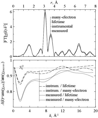
FIG. 5.: Module of the FT of various EXAFS functions: initial; obtained from the instrumentally deconvolved absorptance; the latter was deconvolved with the Lorentzian response and with the total multielectron response, these two give the EXAFS FT’s practically merged. Bottom: the ratio of amplitudes of initial $\chi$ and deconvolved $\chi$. The $S_{0}^{2}$ value was calculated from atomic overlap integrals.

With the specified response functions $W$, perform the Bayesian deconvolution of the absorption coefficient at the optimal regularization parameter, then construct the EXAFS function for which calculate FT and the amplitudes and phases (see figure 5). Just as for the model response in Sec. II, the deconvolution leads to the increase of EXAFS oscillations. As appeared, the deconvolution has practically no influence on the first FT peak originating from the shortest scattering path. It is clear why: the oscillations corresponding to this peak are essentially wider then the response $W$ (for these, $W$ is almost a $\delta$-function), and this is more true for the extended part of a spectrum, due to the period of the oscillations there is even longer (in $E$-space). Thus, it is in the extended part where $\mu$, the solution of equation (1), less differs from $\mu_{\rm m}$.

In modern EXAFS spectroscopy the difference between amplitudes of experimental and calculated spectra are taken into account by the reduction factor $S_{0}^{2}$ which is either treated as a fitting parameter or estimated from the relaxation of the core-hole as the many-electron overlap integral. In many works this factor is considered to be independent from energy, however, as noted in review by Rehr and Albers [11], it must be path-dependent and energy-dependent. At the bottom of figure 5 we draw the ratios $A(k)$ of the amplitude of initial EXAFS spectrum to that of the deconvolved one. Here, they were calculated relatively both $\chi_{\rm m}$ and $\chi_{\rm instr}$. For comparison we show the factor $S_{0}^{2}$ as computed by feff code [12]. At large $k$, where the noise become comparable with the EXAFS signal, the ratios $A(k)$ have significant errors. However, the general trend of the curves corresponds to the expected one [13]: $A(k)$ is minimal at intermediate EXAFS energies, while at both low and high energy $A(k)$ reduces to unity. In addition, there are some phase shifts between the initial spectrum and the deconvolved ones. But these shifts are found to be quite small: less than 0.2 rad at $k<4$ Å and less than 0.1 rad at $k>4$ Å.

The Lorentzian broadening of the EXAFS spectrum with a half-width $\Gamma$ is similar to the effect of the imaginary part of the self-energy with ${\rm Im\,}\Sigma=\Gamma$. The resulting reduction factors, i.e. the ratios the of amplitudes calculated with and without the imaginary part, are analogous to the reduction factors obtained by us relatively $\chi_{\rm instr}$: $A(k)={\rm am}(\chi_{\rm instr})/{\rm am}(\chi_{\rm deconv})$. However, up to now the reduction factors relatively measured EXAFS spectrum were considered, $A(k)={\rm am}(\chi_{\rm m})/{\rm am}(\chi_{\rm deconv})$. As seen (figure 5), these are the noticeably different quantities. That is why for the correct analysis and comparison of spectra taken at different experimental conditions, the instrumental deconvolution must be the first step.

For our example spectrum and the chosen response functions, deconvolution of the lifetime broadening and deconvolution of the multielectron broadening are practically undistinguishable (figure 5, top), i.e. the secondary weak peak in the excitation spectrum $W(\Delta E)$ has very little effect. The main effect of using real excitation spectra is expected from the presence and taking into account the plasmon losses which have a considerable integral weight (figure 1). Because of their very broad spectral distribution, their effect consists in the change of the EXAFS spectrum as a whole. In the present paper this contribution was not taken into account for lack of appropriate experimental information.

Near the absorption edge, where the photoelectron kinetic energy is low, the core-hole relaxation processes are of certain importance for the photoelectron propagation. Here we do not consider the validity of the neglect of this effect, but refer to the review [11].

V Conclusion

To take into account the many-electron effects, there exist, in principle, two approaches: (a) to include into a one-electron theory relevant amendments or (b) to extract a one-electron absorptance from the total one and to use then a pure one-electron theory. The first, traditional, approach invokes semi-empirical rules, but not ab initio calculations, to construct the exchange correlation part of the scattering potential, with the empiricism being based on the comparison with experimental spectra already broadened. In the present paper we have shown the principle way for the second approach, using the solution of integral convolution equation, the kernel in which is the excitation spectrum measured in XPS spectroscopy. Notice, that owing to the specific way of the structural information extraction from the EXAFS spectra, in which an isolated signal in $r$-space or a filtered signal in $k$-space is used, we have not committed a sin against the fact that the integral convolution equation is an ill-posed problem, because from the infinitely large number of solutions it is possible to determine an optimal range, also infinitely large, of solutions any one from which is appropriate.

Because of some technical difficulties, it is impossible so far to measure XPS spectra near deep core levels. Therefore, the desirable pure one-electron absorptance is unavailable. Nevertheless, as we have shown, it is possible to perform an accurate instrumental deconvolution and deconvolution of the lifetime broadening. These procedures make the comparison between calculated and experimental spectra more immediate and the final results of EXAFS spectroscopy more reliable.

All the stages of EXAFS spectra processing including those described here are realized in the freeware program viper [14].