Parametric autoresonance

Abstract

We investigate parametric autoresonance: a persisting phase locking which occurs when the driving frequency of a parametrically excited nonlinear oscillator slowly varies with time. In this regime, the resonant excitation is continuous and unarrested by the oscillator nonlinearity. The system has three characteristic time scales, the fastest one corresponding to the natural frequency of the oscillator. We perform averaging over the fastest time scale and analyze the reduced set of equations analytically and numerically. Analytical results are obtained by exploiting the scale separation between the two remaining time scales which enables one to use the adiabatic invariant of the perturbed nonlinear motion.

]

I INTRODUCTION

This work addresses a combined action of two mechanisms of resonant excitation of (classical) nonlinear oscillating systems. The first is parametric resonance. The second is autoresonance.

There are numerous oscillatory systems which interaction with the external world amounts only to a periodic time dependence of their parameters. The corresponding resonance is called parametric [1, 2]. A textbook example is a simple pendulum with a vertically oscillating point of suspension [1]. The main resonance occurs when the excitation frequency $\omega$ is nearly twice the natural frequency of the oscillator $\omega_{0}$ [1, 2]. Applications of this basic phenomenon in physics and technology are ubiquitous.

Autoresonance occurs in nonlinear oscillators driven by a small external force, almost periodic in time. If the force is exactly periodic, and in resonance with the natural frequency of the oscillator, the resonance region of the phase plane has a finite (and relatively small) width [3, 4]. If instead the driving frequency is slowly varying in time (in the right direction determined by the nonlinearity sign), the oscillator can stay phase-locked despite the nonlinearity. This leads to a continuous resonant excitation. Autoresonance has found many applications. It was extensively studied in the context of relativistic particle acceleration: in the 40-ies by McMillan [5], Veksler [6] and Bohm and Foldy [7, 8], and more recently [9, 10, 11, 12]. Additional applications include a quasiclassical scheme of excitation of atoms [13] and molecules [14], excitation of nonlinear waves [15, 16], solitons [17, 18], vortices [19, 20] and other collective modes [21] in fluids and plasmas, an autoresonant mechanism of transition to chaos in Hamiltonian systems [22, 23], etc.

Until now autoresonance was considered only in systems executing externally driven oscillations. In this work we investigate autoresonance in a parametrically driven oscillator.

Our presentation will be as follows. In Section 2 we briefly review the parametric resonance in non-linear oscillating systems. Section 3 deals, analytically and numerically, with parametric autoresonance. The conclusions are presented in Section 4. Some details of derivation are given in Appendices A and B.

II PARAMETRIC RESONANCE WITH A CONSTANT DRIVING FREQUENCY

The parametric resonance in a weakly nonlinear oscillator with finite dissipation and detuning is describable by the following equation of motion [2, 24, 25]:

$$\ddot{x}+2\gamma\dot{x}+\left[1+\epsilon\cos\left((2+\delta)t\right)\right]x-\beta x^{3}=0.$$ (1)

where the units of time are chosen in such a way that the scaled natural frequency of the oscillator in the small-amplitude limit is equal to 1. In Eq. (1) $\epsilon$ is the amplitude of the driving force, which is assumed to be small: $0<\epsilon\ll 1$, $\delta\ll 1$ is the detuning parameter, $\gamma$ is the (scaled) damping coefficient $(0<\gamma\ll 1)$ and $\beta$ is the nonlinearity coefficient. For concreteness we assume $\beta>0$ (for a pendulum $\beta=1/6$).

Working in the limit of weak nonlinearity, dissipation and driving, we can employ the method of averaging [2, 3, 26, 27], valid for most of the initial conditions [3, 4]. The unperturbed oscillation period is the fast time. Putting $x=a(t)\cos\theta(t)$ and $\dot{x}=-a(t)\sin\theta(t)$ and performing averaging over the fast time, we arrive at the averaged equations

$$\dot{a} = -\gamma a+\frac{\epsilon a}{4}\sin 2\psi,$$ (2)

$$\dot{\psi} = -\frac{\delta}{2}-\frac{3\beta a^{2}}{8}+\frac{\epsilon}{4}\cos 2\psi,$$ (3)

where a new phase $\psi=\theta-[(2+\delta)/2]t$ has been introduced. The averaged system (3) is an autonomous dynamical system with two degree of freedom and therefore integrable. In the conservative case $\gamma=0$ Eqs. (3) become:

$$\dot{a} = \frac{\epsilon a}{4}\sin 2\psi,$$ (4)

$$\dot{\psi} = -\frac{\delta}{2}-\frac{3\beta a^{2}}{8}+\frac{\epsilon}{4}\cos 2\psi.$$ (5)

As $\sin 2\psi$ and $\cos 2\psi$ are periodic functions of $\psi$ with a period $\pi$, it is sufficient to consider the interval $-\pi/2<\psi\leq\pi/2$. For small enough detuning, $\delta<\epsilon/2$, there is an elliptic fixed point with a non-zero amplitude:

$$a_{*}=\pm\left[\frac{2\epsilon}{3\beta}\left(1-\frac{2\delta}{\epsilon}\right)\right]^{1/2};\indent\psi_{*}=0.$$

We need to calculate the period of motion in the phase plane along a closed orbit around this fixed point (such an orbit is shown in Fig. 1).

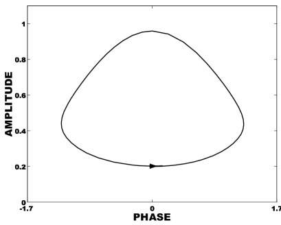
FIG. 1.: Parametric resonance with a constant driving frequency. Shown is a typical closed orbit in the phase plane with period $T$ ($\epsilon=0.04,\delta=-0.04,\beta=1/6$ and $\gamma=0.$). For a time-dependent driving frequency $\nu(t)$, the autoresonance will occur if the characteristic time for variation of $\nu(t)$ is much greater than $T$, see criterion (14).

This calculation was performed by Struble [24]. For a zero detuning, $\delta=0$, Hamilton’s function (we will call it the Hamiltonian) of the system (5) is the following:

$$H(I,\psi)=\frac{\epsilon I}{4}\cos 2\psi-\frac{3\beta I^{2}}{8}=H_{0}=const.,$$ (6)

where we have introduced the action variable $I=a^{2}/2$. Solving Eq. (6) for $I$ and substituting the result into the Hamilton’s equation for $\dot{\psi}$ we obtain:

$$\dot{\psi}=\mp\frac{\epsilon}{4}\left(\cos^{2}2\psi-\frac{24\beta H_{0}}{\epsilon^{2}}\right)^{1/2},$$ (7)

where the minus (plus) sign corresponds to the upper (lower) part of the closed orbit. The period of the amplitude and phase oscillations is therefore

$$T=\frac{8}{\epsilon}\int_{-\overline{\psi}}^{\overline{\psi}}\frac{d\psi}{\left(\cos^{2}2\psi-\frac{24\beta H_{0}}{\epsilon^{2}}\right)^{1/2}},$$ (8)

where $-\overline{\psi}$ and $\overline{\psi}$ are the roots of the equation $\cos^{2}2\psi=24\beta H_{0}/\epsilon^{2}.$ Calculating the integral, we obtain

$$T=\frac{8}{\epsilon}K(m),$$ (9)

where $K(m)$ is the complete elliptic integral of the first kind [28], and $m=1-24\beta H_{0}/\epsilon^{2}$. This result will be used in Section 3 to establish a necessary condition for the parametric autoresonance to occur.

III PARAMETRIC RESONANCE WITH A TIME-DEPENDENT DRIVING FREQUENCY: PARAMETRIC AUTORESONANCE

Now let the driving frequency vary with time. This time dependence introduces an additional (third) time scale into the problem. The governing equation becomes

$$\ddot{x}+2\gamma\dot{x}+(1+\epsilon\cos\phi)x-\beta x^{3}=0,$$ (10)

where $\dot{\phi}=\nu(t)$. We will assume $\nu(t)$ to be a slowly decreasing function which initial value is $\nu(t=0)=2+\delta.$ Using the scale separation, we obtain the averaged equations. The averaging procedure of Section 2 can be repeated by replacing $(2+\delta)t$ by $\phi$ in all equations. There is one new point that should be treated more accurately. The averaging procedure is applicable (again, for most of the initial conditions) if there is a separation of time scales. It requires, in particular, a strong inequality $2\dot{\theta}+\nu(t)\gg 2\dot{\theta}-\nu(t)$. This inequality can limit the time of validity of the method of averaging. Let us assume, for concreteness, a linear frequency “chirp”:

$$\nu(t)=2+\delta-2\mu t,$$ (11)

where $\mu\ll 1$ is the chirp rate. In this case the averaging procedure is valid as long as $\mu t\ll 1$.

Introducing a new phase $\psi=\theta-\phi/2$, we obtain a reduced set of equations (compare to Eqs. (3)):

$$\dot{a} = -\gamma a+\frac{\epsilon a}{4}\sin 2\psi,$$ (12)

$$\dot{\psi} = -\frac{\delta}{2}+\mu t-\frac{3\beta a^{2}}{8}+\frac{\epsilon}{4}\cos 2\psi.$$ (13)

The first of Eqs. (13) is typical for parametric resonance: to get excitation one should start from a non-zero oscillation amplitude. As we will see, the $\mu t$ term in the second of Eqs. (13) (when small enough and of the right sign) provides a continuous phase locking, similar to the externally driven autoresonance.

Consider a numerical example. Fig. 2 shows the time dependence $a(t)$ found by solving Eqs.  (13) numerically. One can see that the system remains phase locked which allows the amplitude of oscillations to increase, on the average, with time in spite of the nonlinearity. The time-dependence of the amplitude includes a slow trend and relatively fast, decaying oscillations. These are the two time scales remaining after the averaging over the fastest time scale.

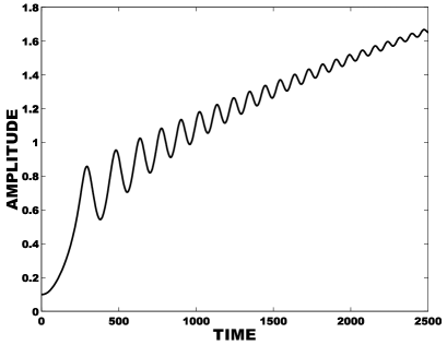
FIG. 2.: An example of parametric autoresonance. Shown is the oscillation amplitude versus time, computed numerically from the averaged equations (13). The system remains phase-locked which allows the amplitude to increase, on the average, with time. The parameters are $\mu=6.5\cdot 10^{-5},\epsilon=0.04,\delta=-0.01,\beta=1/6$ and $\gamma=0.001$.

Similar to the externally-driven autoresonance, a persistent growth of the oscillation amplitude requires the characteristic time of variation of $\nu(t)$ to be much greater than the “nonlinear” period $T$ [see Eq. (9)] of oscillations of the amplitude:

$$\left|\frac{\nu(t)}{\dot{\nu}(t)}\right|\gg T.$$ (14)

Like its externally-driven analog, the parametric autoresonance is insensitive to the exact form of $\nu(t)$. For a given set of parameters, the optimal chirping rate can be found: too low a chirping rate means an inefficient excitation, while too high a rate leads to phase unlocking and termination of the excitation.

In the remainder of the paper we will develop an analytical theory of the parametric autoresonance. The first objective of this theory is a description of the slow trend in the amplitude (and phase) dynamics. When the driving frequency $\nu$ is constant, there is an elliptic fixed point $a_{*}$ (see Section 2). When $\nu$ varies with time, the fixed point ceases to exist. However, for a slowly-varying $\nu(t)$ one can define a “quasi-fixed” point $a_{*}(t)$ which is a slowly varying function of time. It is this quasi-fixed point that represents the slow trend seen in Fig. 2 and corresponds to an “ideal” phase-locking regime. The fast, decaying oscillations seen in Fig. 2 correspond to oscillations around the quasi-fixed point in the phase plane [this phase plane is actually projection of the extended phase space ($a,\psi,t$) on the ($a,\psi$)-plane].

In the main part of this Section we neglect the dissipation and use a Hamiltonian formalism. First we will consider excitation in the vicinity of the quasi-fixed point. Then excitation from arbitrary initial conditions will be investigated. Finally, the role of dissipation will be briefly analyzed.

For a time-dependent $\nu(t)$, the Hamiltonian becomes [compare to Eq. (6)]:

$$H(I,\psi,t)=\frac{\epsilon I}{4}\left(\alpha(t)+\cos 2\psi\right)-\frac{3\beta I^{2}}{8},$$ (15)

where $\alpha(t)=(4/\epsilon)(1-\nu(t)/2).$ The Hamilton’s equations are:

$$\dot{I} = \frac{\epsilon I}{2}\sin 2\psi,$$ (16)

$$\dot{\psi} = \frac{\epsilon}{4}\left(\alpha+\cos 2\psi\right)-\frac{3\beta I}{4}.$$ (17)

Let us find the quasi-fixed point of (17), i.e. the special autoresonance trajectory $I_{*}(t),\,\psi_{*}(t)$ corresponding to the “ideal” phase locking (a pure trend without oscillations).

Assuming a slow time dependence, we put $\dot{\psi_{*}}=0$, that is

$$\frac{\epsilon}{4}\left(\alpha+\cos 2\psi_{*}\right)-\frac{3\beta I_{*}}{4}=0.$$ (18)

Differentiating it with respect to time and using Eqs. (17), we obtain an algebraic equation for $\psi_{*}(t)$:

$$2\alpha(t)\sin 2\psi_{*}+\sin 4\psi_{*}=\frac{16\mu}{\epsilon^{2}}.$$ (19)

At this point we should demand that $\dot{\psi_{*}}(t)$, evaluated on the solution of Eq. (19), is indeed negligible compared to the rest of terms in the equation (17) for $\dot{\psi}(t)$. It is easy to see that this requires $16\mu/\epsilon^{2}\ll 1$. In this case the sines in Eq. (19) can be replaced by their arguments, and we obtain the following simple expressions for the quasi-fixed point:

$$I_{*} \simeq \frac{\epsilon}{3\beta}\left(\alpha+1\right)\,,$$ (20)

$$\psi_{*} \simeq \frac{k}{\alpha+1}\,,$$ (21)

where $k=4\mu/\epsilon^{2}$.

A Excitation in the vicinity of the quasi-fixed point

Let us make the canonical transformation from variables $I$ and $\psi$ to $\delta I=I-I_{*}$ and $\delta\psi=\psi-\psi_{*}.$ Assuming $\delta I$ and $\delta\psi$ to be small and keeping terms up to the second order in $\delta I$ and $\delta\psi$, we obtain the new Hamiltonian:

$$H(\delta I,\delta\psi,\alpha(t)) = -\frac{\epsilon k}{\alpha+1}\delta I\delta\psi-$$ (22)

$$- \frac{3\beta}{8}(\delta I)^{2}-\frac{\epsilon^{2}}{6\beta}(\alpha+1)(\delta\psi)^{2}\,.$$ (23)

Here and in the following small terms of order of $k^{2}$ are neglected. Let us start with the calculation of the local maxima of $\delta I(t)$ and $\delta\psi(t)$, which will be called $\delta I_{max}(t)$ and $\delta\psi_{max}(t)$, respectively. As $\alpha(t)$ is a slow function of time [so that the strong inequality (14) is satisfied], we can exploit the approximate constancy of the adiabatic invariant [1, 29]:

$$J=\frac{1}{2\pi}\oint\delta Id(\delta\psi)\simeq const.$$ (24)

$|J|$ is the area of the ellipse defined by Eq. (23) with the time-dependencies “frozen”. Therefore,

$$J=\frac{2}{\epsilon}\frac{H}{(\alpha+1)^{1/2}}\simeq const.$$ (25)

This expression can be rewritten in terms of $\delta I$ and $\delta\psi$:

$$|J| = \frac{2k}{(\alpha+1)^{3/2}}\delta I\delta\psi+\frac{3\beta}{4\epsilon}\frac{1}{(\alpha+1)^{1/2}}(\delta I)^{2}$$ (26)

$$+ \frac{\epsilon}{3\beta}(\alpha+1)^{1/2}(\delta\psi)^{2}.$$ (27)

If $k=4\mu/\epsilon^{2}\ll 1$, the term with $\delta I\delta\psi$ in (27) can be neglected (in this approximation one has $\psi_{*}=0$). Then $J$ becomes a sum of two non-negative terms, one of them having the maximum value when the other one vanishes. Therefore,

$$\delta I_{max}(t)=2\left(\frac{\epsilon J}{3\beta}\right)^{1/2}\left(\alpha+1\right)^{1/4},$$ (28)

and

$$\delta\psi_{max}(t)=\left(\frac{3\beta J}{\epsilon}\right)^{1/2}\frac{1}{(\alpha+1)^{1/4}}.$$ (29)

Now we calculate the period of oscillations of the action and phase. Using the well-known relation [1] $T=2\pi(\partial J/\partial H)$, we obtain from Eq. (25):

$$T=\frac{4\pi}{\epsilon}\frac{1}{(\alpha+1)^{1/2}}.$$ (30)

The period of oscillations versus time is shown in Fig. 3. The theoretical curve [Eq. (30)] shows an excellent agreement with the numerical solution.

Now we obtain the complete solution $\delta I(t)$ and $\delta\psi(t)$. The Hamilton’s equations corresponding to the Hamiltonian (23) are:

$$\dot{\delta I} = \frac{\epsilon^{2}}{3\beta}\left(\alpha+1\right)\delta\psi+\frac{\epsilon k}{\alpha+1}\delta I,$$ (31)

$$\dot{\delta\psi} = -\frac{3\beta}{4}\delta I-\frac{\epsilon k}{\alpha+1}\delta\psi.$$ (32)

Differentiating the second equation with respect to time and substituting the first one, we obtain a linear differential equation for $\delta\psi(t)$:

$$\ddot{\delta\psi}+\omega^{2}(t)\delta\psi=0,$$ (33)

where $\omega(t)=(\epsilon/2)(\alpha(t)+1)^{1/2}$. For the linear $\nu(t)$ dependence (Eq. (11)) we have $\alpha(t)=4\mu t/\epsilon-2\delta/\epsilon$, therefore for $k\ll 1$ the criterion $\dot{\omega}/\omega^{2}\ll 1$ is satisfied, and Eq. (33) can be solved by the WKB method (see, e.g. [4]).

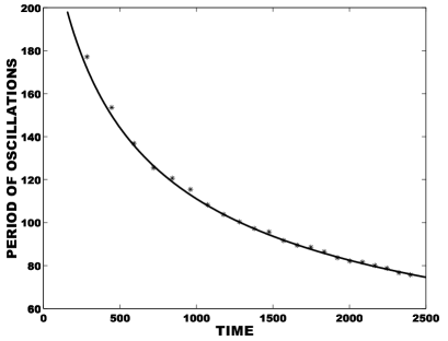
FIG. 3.: Excitation in the vicinity of the quasi-fixed point: the time-dependence of the period $T$ of the action and phase oscillations. The solid line is the theoretical curve, Eq. (30), the asterisks are points obtained numerically. The parameters are $\mu=6.5\cdot 10^{-5},\epsilon=0.04,\delta=-0.01$ and $\beta=1/6$.

The WKB solution takes the form (details are given in Appendix A):

$$\delta\psi(t) = \left(\frac{3\beta J}{\epsilon}\right)^{1/2}\frac{1}{(\alpha+1)^{1/4}}$$ (34)

$$\times \cos\left(q_{0}+\frac{(\alpha+1)^{3/2}}{3k}\right),$$ (35)

where the phase $q_{0}$ is determined by the initial conditions. The full solution for the phase is $\psi=\delta\psi+\psi_{*}$ and Fig.  4 compares it with a numerical solution of Eq. (17). Also shown are the minimum and maximum phase deviations predicted by Eqs. (29) and (21). One can see that the agreement is excellent.

The solution for $\delta I(t)$ can be obtained by substituting Eq. (35) into the second equation of the system (32). In the same order of accuracy (see Appendix A)

$$\delta I(t)=2\left(\frac{\epsilon J}{3\beta}\right)^{1/2}\left(\alpha+1\right)^{1/4}\sin\left(q_{0}+\frac{(\alpha+1)^{3/2}}{3k}\right)\,.$$ (36)

Fig. 5 shows the dependence of the action variable with the trend $I_{*}(t)$ subtracted, $\delta I(t)$, on time predicted by Eq. (36), and found from the numerical solution. It also shows the minimum and maximum action deviations (28). Again, a very good agreement is obtained.

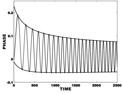
FIG. 4.: Parametric autoresonance excitation in the vicinity of the quasi-fixed point. Shown is the phase $\psi(t)$ found analytically [Eqs. (21) and (35)] and by solving Eq. (17) numerically. The analytical and numerical curves are indistinguishable. Also shown are the minimum and maximum phase deviations predicted by Eq. (29) and (21). The parameters are the same as in Fig. 3.

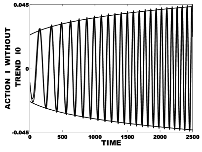
FIG. 5.: Parametric autoresonance excitation in the vicinity of the quasi-fixed point. Shown is the action variable $\delta I(t)$ from Eq. (36) and from the numerical solution. Also shown are the minimum and maximum action deviations predicted by Eq. (28). The parameters are the same as in Fig. 3.

B Excitation from arbitrary initial conditions

In this Subsection we go beyond the close vicinity of the quasi-fixed point and calculate the maximum deviations of the action $I$ and phase $\psi$ for arbitrary initial conditions. Again, these calculations are made possible by employing the adiabatic invariant for the general case. Correspondingly, the period of the action and phase oscillations will be also calculated.

Let us first express the maximum and minimum action deviations in terms of the Hamiltonian $H$ and driving frequency $\nu(t)$. Solving Eq. (15) as a quadratic equation for $I$, we obtain:

$$I_{1,2}=\frac{\epsilon}{3\beta}\left(\alpha+\cos 2\psi\right)\pm\left[\frac{\epsilon^{2}}{9\beta^{2}}\left(\alpha+\cos 2\psi\right)^{2}-\frac{8H}{3\beta}\right]^{1/2}.$$

The time derivative of $I$ vanishes when $I=I_{max}$ or $I=I_{min}$. Therefore, from the first equation of the system (17) $\psi=0$ so that

$$I_{max,min}=\frac{\epsilon}{3\beta}\left(\alpha+1\right)\pm\left[\frac{\epsilon^{2}}{9\beta^{2}}\left(\alpha+1\right)^{2}-\frac{8H_{up,down}}{3\beta}\right]^{1/2},$$ (37)

where $H_{up,down}=H(I_{max,min},\psi=0)$.

Now we express the maximum and minimum phase deviations through the Hamiltonian $H$ and driving frequency $\nu(t)$. The time derivative $\dot{\psi}$ vanishes if $\psi=\psi_{max}$ or $\psi=\psi_{min}$, then the second equation of the system  (17) yields $I=(\epsilon/3\beta)(\alpha+\cos 2\psi)$. In this case the Hamiltonian (15) becomes $H_{right,left}=(\epsilon^{2}/24\beta)(\alpha+\cos 2\psi_{max,min})^{2}$. Finally, the expression for $\psi_{max,min}$ is

$$\psi_{max,min}=\pm\frac{1}{2}\arccos\left[\left(\frac{24\beta H_{right,left}}{\epsilon^{2}}\right)^{1/2}-\alpha\right]\,.$$ (38)

Fig. 6 shows a part of a typical autoresonant orbit in the phase plane. For $\nu(t)=const.$ this orbit is determined by the equation $H(I,\psi,\nu)=const.$, and it is closed. As in our case $\nu(t)$ changes with time, the trajectory is not closed. To calculate the maximum and minimum deviations of action and phase we should know the values of the Hamiltonian at 4 points of the orbit that we will call “up”, “down”, “left”, and “right” in the following.

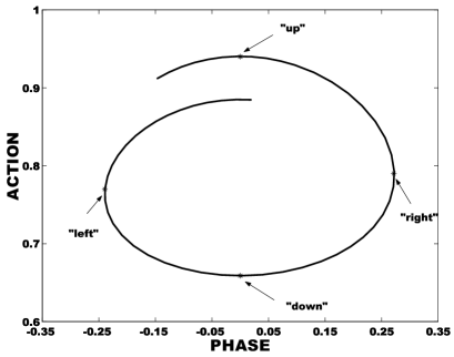
FIG. 6.: A part of the autoresonant orbit in the phase plane. Knowing the Hamiltonian at the 4 points, we can calculate the maximum and minimum deviations of the action and phase. The parameters are the same as in Fig. 3.

Knowing the values of the Hamiltonian at these 4 points, we calculate $I_{max,min}$ from Eq. (37) and $\psi_{max,min}$ from Eq. (38). Figs. (7) and (8) show these deviations for action and phase correspondingly, and the values of $I$ and $\psi$, found from numerical solution. The theoretical and numerical results show an excellent agreement.

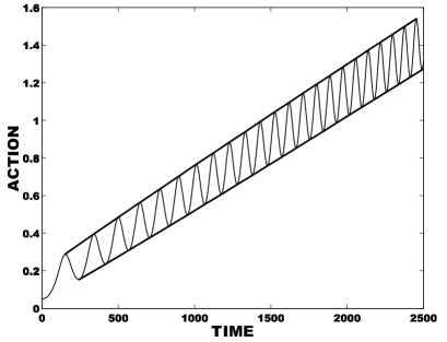
FIG. 7.: The maximum and minimum deviations of the action, calculated from Eq. (37) (thick line) and from numerical solution (thin line). The parameters are the same as in Fig. 3.

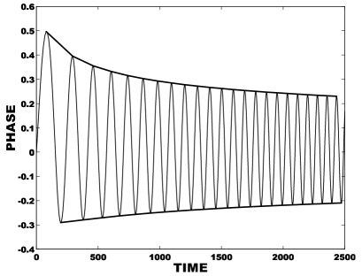
FIG. 8.: The maximum and minimum deviations of the phase, calculated from Eq. (38) (thick line) and from numerical solution (thin line). The parameters are the same as in Fig. 3.

Now we are prepared to calculate the adiabatic invariant $J(H,\nu(t))$. Its (approximate) constancy in time allows one, in principle, to find the Hamiltonian $H(t)$ at any time $t$, in particular at the points of the maximum and minimum action and phase deviations (see Fig. 6).

It is convenient to rewrite the adiabatic invariant in the following form:

$$J=\frac{1}{2\pi}\oint\psi dI.$$ (39)

Using Eq. (15), we can find $\psi=\psi(H,I,\alpha(t))$:

$$\psi=\pm\frac{1}{2}\arccos\left(\frac{8H+3\beta I}{2\epsilon I}-\alpha\right)\,,$$ (40)

so that Eq. (39) becomes:

$$J=\frac{1}{2\pi}\int^{I_{max}}_{I_{min}}\arccos\left(\frac{8H+3\beta I}{2\epsilon I}-\alpha\right)dI,$$ (41)

where $I_{max}$ and $I_{min}$ are given by Eq. (37). Notice that $H(t)$ and $\alpha(t)$ should be treated as constants under the integral (41), see Refs. [1, 3, 29]. This integral can be expressed in terms of elliptic integrals (see Appendix B for details). For definiteness, we used the values of $H(t)$ and $\alpha(t)$ in the “up” points, see Fig. 6. We checked numerically that the adiabatic invariant $J(H(t),\alpha(t))$ is constant in our example within 0.12 per cent.

Now we calculate the period of action and phase oscillations. From the first equation of system  (17) we have:

$$T=2\int^{I_{max}}_{I_{min}}\frac{dI}{(\epsilon I/2)\sin 2\psi},$$ (42)

where $I_{max}$ and $I_{min}$ are given by Eq. (37), while $\psi=\psi(I)$ is defined by (40).

Using Eq. (15), we obtain after some algebra:

$$T=\frac{8}{3\beta}\int^{I_{max}}_{I_{min}}\frac{dI}{G(I)^{1/2}},$$ (43)

where $G(I)$ is given in Appendix B, Eq. (B2). Again, we treat $H(t)$ and $\alpha(t)$ as constants under the integral (43), and take their values in the “right” points, see Fig. 6. The final result is:

$$T=C_{2}K(C_{3}),$$ (44)

where $C_{2}=4(2/3\beta H\epsilon^{2})^{1/4}$ and

$$C_{3}=\frac{1}{2}-\frac{C_{2}^{2}}{16}\left[\frac{3\beta H}{2}+\frac{\epsilon^{2}}{16}\left(1-\alpha^{2}\right)\right]\,.$$

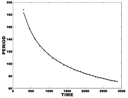
FIG. 9.: The period $T$ of the phase (action) oscillations obtained from Eq. (44) (solid line), and from numerical solution (asterisks). The parameters are the same as in Fig. 3.

Figure 9 shows the period $T$ of the phase and action oscillations versus time obtained analytically and from numerical solution. This completes our consideration of the parametric autoresonance without dissipation.

C Role of dissipation

Now we very briefly consider the role of dissipation in the parametric autoresonance. Consider the averaged equations (13) and assume that the detuning is zero. The non-trivial quasi-fixed point exists when the dissipation is not too strong: $\gamma<\epsilon/4$, and it is given by

$$a_{*} = \left(\frac{2\epsilon}{3\beta}\right)^{1/2}\left[\alpha(t)+\left(1-\frac{16\gamma^{2}}{\epsilon^{2}}\right)^{1/2}\right]^{1/2},$$ (45)

$$\psi_{*} = \frac{1}{2}\arcsin\left(\frac{4\gamma}{\epsilon}+\frac{2k}{\alpha(t)+(1-16\gamma^{2}/\epsilon^{2})^{1/2}}\right)\,.$$ (46)

Again, we assume $k\ll 1$. This quasi-fixed point describes the slow trend in the dissipative case. As we see numerically, fast oscillations around the trend, $\delta a=a-a_{*}$ and $\delta\psi=\psi-\psi_{*}$ decay with time. Therefore, one can expect that the $a(t)$ will approach, at sufficiently large times, the trend $a_{*}(t)$. Fig. 10 shows the time dependence of the amplitude, found by solving numerically the system of averaged equations (13), and the amplitude trend from (46). We can see that indeed the amplitude $a(t)$ approaches the trend $a_{*}(t)$ at large times.

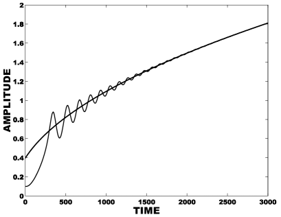
FIG. 10.: Parametric autoresonance with dissipation: the time dependence of the amplitude of oscillations, obtained from numerical solution of Eqs. (13), and the amplitude trend $a_{*}(t)$, predicted by Eq. (46). The parameters are $\mu=6.5\cdot 10^{-5},\epsilon=0.04,\delta=0,\gamma=0.002$ and $\beta=1/6$.

Therefore, a small amount of dissipation enhances the stability of the parametric autoresonance excitation scheme. A similar result for the externally-driven autoresonance was previously known [30].

IV CONCLUSIONS

We have investigated, analytically and numerically, a combined action of two mechanisms of resonant excitation of nonlinear oscillating systems: parametric resonance and autoresonance. We have shown that parametric autoresonance represents a robust and efficient method of excitation of nonlinear oscillating systems. Parametric autoresonance can be extended for the excitation of nonlinear waves. We expect that parametric autoresonance will find applications in different fields of physics.

A CALCULATION OF PHASE AND ACTION DEVIATIONS BY THE WKB-METHOD

Changing the variables from time $t$ to $\alpha$, we can rewrite Eq. (33) in the following form:

$$\delta\psi^{\prime\prime}+\left(\frac{\alpha(t)+1}{4k^{2}}\right)\delta\psi=0\,,$$ (A1)

where ^′′ denotes the second derivative with respect to $\alpha$. Solving this equation by the WKB-method [4], we obtain for $\delta\psi$:

$$\delta\psi(t)=\frac{(2kC)^{1/2}}{(\alpha+1)^{1/4}}\cos\left(\Omega_{0}+\frac{(\alpha(t)+1)^{3/2}-1}{3k}\right),$$ (A2)

where $\Omega_{0}$ and $C$ are constants to be found later. Now we obtain the solution for $\delta I$. Substituting (A2) into the second equation of the system (32), we obtain in the same order of accuracy:

$$\delta I(t) = \frac{2\epsilon}{3\beta}\left(2kC\right)^{1/2}\left(\alpha+1\right)^{1/4}$$ (A3)

$$\times \sin\left(\Omega_{0}+\frac{(\alpha(t)+1)^{3/2}-1}{3k}\right).$$ (A4)

The constant $C$ can be expressed through the adiabatic invariant $J$, given by (27). From Eqs. (A2) and (A4) we have:

$$2kC=\left(\frac{3\beta}{2\epsilon}\right)^{2}\frac{1}{(\alpha+1)^{1/2}}\left(\delta I\right)^{2}+\left(\alpha+1\right)^{1/2}(\delta\psi)^{2}.$$

Comparing it with (27) we find: $C\simeq 3\beta J/2k\epsilon.$ Substituting this value into Eqs. (A2) and (A4) we obtain the final expressions (35) and (36) for $\delta\psi(t)$ and $\delta I(t)$.

B CALCULATION OF THE ADIABATIC INVARIANT

After integration by parts and some algebra, using Eqs. (15) and  (37), we obtain the following expression for the adiabatic invariant:

$$J=\frac{1}{2\pi}\int^{I_{max}}_{I_{min}}\left(\frac{I^{2}-\frac{8H}{3\beta}}{G(I)^{1/2}}\right)dI,$$ (B1)

where

$$G(I)=\left(I_{max}-I\right)\left(I-I_{min}\right)\left[\left(I+\frac{\epsilon(1-\alpha)}{3\beta}\right)^{2}-\frac{16D}{9\beta^{2}}\right],$$ (B2)

and we assume $D=(\epsilon^{2}/16)(1-\alpha)^{2}-3\beta H/2<0.$ Calculation of this integral employs several changes of variable shown in the best way by Fikhtengolts [31]. Using the reduction formulas [28], we arrive at:

$$J=C_{1}\left[\frac{1+mm^{\prime}}{(1-m)^{2}(1+m^{\prime})}\Pi\left(\frac{m}{m-1}\backslash k^{2}\right)\right.$$ (B3)

$$\left.-\frac{1}{1-m}K\left(k^{2}\right)+\frac{m+m^{\prime}}{(1-m)(1+m^{\prime})}E\left(k^{2}\right)\right],$$ (B4)

where

$$m=\frac{(\epsilon/3\beta)(1+\alpha)-(8H/3\beta)^{1/2}}{(\epsilon/3\beta)(1+\alpha)+(8H/3\beta)^{1/2}}>0,$$

$$m^{\prime}=\frac{(\epsilon/3\beta)(1-\alpha)+(8H/3\beta)^{1/2}}{-(\epsilon/3\beta)(1-\alpha)+(8H/3\beta)^{1/2}}>0.$$

$$k^{2}=\frac{m}{m+m^{\prime}},\indent C_{1}=c\cdot\frac{64H}{3\beta(m+m^{\prime})^{1/2}},$$

and

$$c = \frac{1}{2\pi}\left[\frac{\epsilon}{3\beta}\left(1+\alpha\right)+\left(\frac{8H}{3\beta}\right)^{1/2}\right]^{-1/2}$$ (B5)

$$\times \left[-\frac{\epsilon}{3\beta}\left(1-\alpha\right)+\left(\frac{8H}{3\beta}\right)^{1/2}\right]^{-1/2}\,.$$ (B6)

Here $K$, $E$ and $\Pi$ are the complete elliptic integrals of the first, second and third kind, respectively.

REFERENCES

- [1] L.D. Landau and E.M. Lifshits, Mechanics (Pergamon Press, Oxford, 1976).
- [2] N.N. Bogolubov and Y.A. Mitropolsky, Asymptotic Methods In The Theory of Non-linear Oscillations (Gordon and Breach Science Publishers, New York, 1961).
- [3] R.Z. Sagdeev, D.A. Usikov, and G.M. Zaslavsky, Nonlinear Physics (Harwood Academic, Switzerland, 1988).
- [4] A.J. Lichtenberg and M.A. Lieberman, Regular and Chaotic Dynamics (Springer-Verlag, Oxford, 1992).
- [5] E.M. McMillan, Phys. Rev. 68, 143 (1945).
- [6] V. Veksler, J.Phys.(USSR) 9, 153 (1945).
- [7] D. Bohm and L. Foldy, Phys. Rev. 70, 249 (1947).
- [8] D. Bohm and L. Foldy, Phys. Rev. 72, 649 (1947).
- [9] K.S. Golovanivsky, Phys. Scripta 22, 126 (1980).
- [10] B. Meerson, Phys. Lett. A 150, 290 (1990).
- [11] B. Meerson and T. Tajima, Optics Communications 86, 283 (1991).
- [12] L. Friedland, Phys. Plasmas 1, 421 (1994).
- [13] B. Meerson and L. Friedland, Phys. Rev. A 41, 5233 (1990).
- [14] J.M. Yuan and W.K. Liu, Phys. Rev. A 57, 1992 (1998).
- [15] M. Deutsch, B. Meerson, and J.E. Golub, Phys. Fluids B 3, 1773 (1991).
- [16] L. Friedland, Phys. Plasmas 5, 645 (1998).
- [17] I. Aranson, B. Meerson, and T. Tajima, Phys. Rev. A 45, 7500 (1992).
- [18] L. Friedland and A. Shagalov, Phys. Rev. Lett. 81, 4357 (1998).
- [19] L. Friedland, Phys. Rev. E 59, 4106 (1999).
- [20] L. Friedland and A.G. Shagalov, Phys. Rev. Lett. 85, 2941 (2000).
- [21] J. Fajans, E. Gilson, and L. Friedland, Phys. Rev. Lett. 82, 4444 (1999); Phys. Plasmas 6, 4497 (1999).
- [22] B. Meerson and S. Yariv, Phys. Rev. A 44, 3570 (1991).
- [23] G. Cohen and B. Meerson, Phys. Rev. E 47, 967 (1993).
- [24] R.A. Struble, Quart. Appl. Math. 21, 121 (1963).
- [25] A.D. Morozov, J. Appl. Math. Mech. 59, 563 (1995).
- [26] M.I. Rabinovich and D.I. Trubetskov, Oscillations and Waves in Linear and Nonlinear Systems (Kluwer Academic Publisher, Dordrecht, 1989).
- [27] P.G. Drazin, Nonlinear Systems (Cambridge University Press, Cambridge, 1992).
- [28] M. Abramowitz, Handbook of Mathematical Functions (National Bureau of Standards, Washington, 1964).
- [29] H. Goldstein, Classical Mechanics (Addison-Wesley, Reading, Mass., 1980).
- [30] S. Yariv and L. Friedland, Phys. Rev. E 48, 3072 (1993).
- [31] G.M. Fikhtengolts, The Fundamentals of Mathematical Analysis (Pergamon Press, New York, 1965).