On Resonant Multi-Bunch Wakefield Effects in Linear Accelerators with Dipole Mode Detuning

In this report we explore resonant multi-bunch (transverse) wakefield effects in a linear accelerator in which the dipole modes of the accelerator structures have been detuned. For examples we will use the parameters of a slightly simplified version of an optimized S-band structure described in Ref. [1]. Note that we are also aware of a different analysis of resonant multi-bunch wakefield effect[2].

It is easy to understand how resonances can arise in a linac with bunch trains. Consider first the case of the interaction of the beam with one single structure mode. The leading bunch enters the structure offset from the axis and excites the mode. If the bunch train is sitting on an integer resonance, i.e. if $f\Delta t=n$, with $f$ the mode frequency, $\Delta t$ the bunch spacing, and $n$ an integer, then when the 2nd bunch arrives it will excite the mode at the same phase and also obtain a kick due to the wakefield of the first bunch. The $m{\rm th}$ bunch will also excite the mode in the same phase and obtain $(m-1)$ times the kick from the wakefield that the second bunch experienced (for simplicity we assume the mode $Q$ is infinity). On the half-integer resonance, i.e. when $f\Delta t=n+.5$, the $m{\rm th}$ bunch will also receive kicks from the wakefield left by the earlier bunches, but in this case the kicks will alternate in direction, and no resonance builds up. For a transverse wakefield effect, such as we are interested in here, however, this simple description of the resonant interaction needs to be modified slightly. For this case the wake varies as $\sin(2\pi ft)$, and neither the integer nor the half-integer resonance condition will excite any wakefield for the following bunches. In this case resonant growth is achieved at a slight deviation from the condition $f\Delta t=n$, as is shown below.

In the following, for simplicity, we will use the “uncoupled” model to investigate resonant effects in the sum wake for a structure with modes with a uniform frequency distribution. According to this model (see, for example, Ref. [3])

$$W(t)\approx\sum^{N_{c}}_{n}2k_{sn}\sin({2\pi f_{sn}t/c})\quad\quad\quad[t\ {\rm small}],$$ (1)

where $N_{c}$ is the number of cells in the structure, and $f_{sn}$ and $k_{sn}$ are, respectively, the frequency and kick factor at the synchronous point, for a periodic structure with dimensions of cell $n$. Therefore, one can predict the short time behavior of the wake without solving for the eigenmodes of the system. The point of using the uncoupled model is that it allows us to study the effect of an idealized, uniform frequency distribution. As is well known, an ideal (input) frequency distribution becomes distorted by the cell-to-cell coupling of an accelerator structure. (For simplicity we will drop the $s$ in the subscripts for frequency below.) For examples we will use the parameters of a slightly simplified version (all kick factors are equal, the frequency distribution is uniform instead of trapezoidal) of the optimized $3\pi/4$ S-band structure described in Ref. [1]: there are $N_{c}=102$ cells (also modes), the central frequency ${\bar{f}}=3.92$ GHz, and the full-width of the distribution $\Delta_{\delta f}=5.8\%$; for bunch structure we consider the nominal configuration of $M=95$ bunches in a train and a bunch spacing $\Delta t=2.4$ ns. The results for the real structure, with coupled modes, will be slightly different yet qualitatively the same.

Consider first the case of a structure with only one dipole mode, with frequency $f$, and a kick factor that we will normalize (for simplicity) to $1/2$. Suppose there are $M$ bunches in the bunch train. The sum wake at the $m{\rm th}$ bunch is given by

$$S_{m}^{(1)}(f\Delta t) = \sum_{i=1}^{m}\sin\left(2\pi[i-1]f\Delta t\right)$$ (2)

$$= {\sin\left(\pi[m-1]f\Delta t\right)\sin\left(\pi mf\Delta t\right)\over\sin\left(\pi f\Delta t\right)}\quad.$$

As with the nominal (2.8 ns) bunch spacing in the S-band prelinacs, let us, for an example, consider $M=95$ bunches and the region near the 11th harmonic. In Fig. 1 we plot $f\Delta t$ vs the sum wake for the $M$th (the last) bunch, $S_{M}^{(1)}$, near the 11th integer resonance. It can be shown that, if $M$ is not small, the largest resonance peaks (the extrema of the curve) are at

$$f\Delta t\approx n\pm{3\over 8M}\quad\quad[M\ {\rm not\ small}]\quad,$$ (3)

with values $\pm.72M$. Note that at the exact integer and half-integer resonant spacings the sum wake is zero.

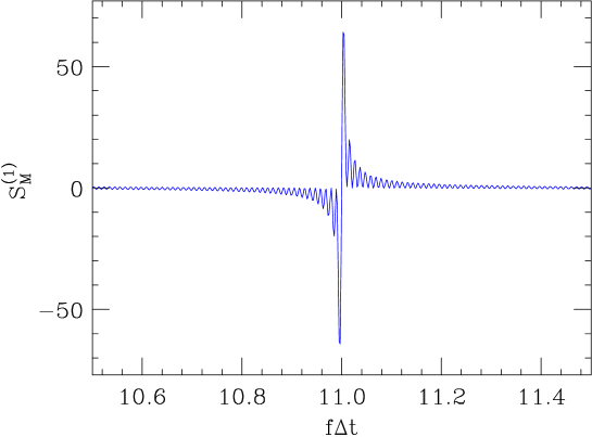
Figure 1: The sum wake at the last bunch in a train vs bunch spacing, due to a single mode (Eq. 2); $M=95$ bunches.

Now let us consider a uniform distribution of mode frequencies. For simplicity we will let all the kick factors be equal, and be normalized to $1/2$. The sum wake, according to the uncoupled model, becomes

$$S_{m}({\bar{f}}\Delta t)={1\over N_{c}}\sum_{n=1}^{N_{c}}S_{m}^{(1)}\left[{\bar{f}}\Delta t\left(1+{(n-N_{c}/2)\over N_{c}}\Delta_{\delta f}\right)\right]\quad,$$ (4)

with $N_{c}$ the number of cells (also the number of modes), $\bar{f}$ the central frequency, and $\Delta_{\delta f}$ the total (relative) width of the frequency distribution. As an example, let us consider the optimized $3\pi/4$ S-band structure, with $N_{c}=102$ and $\Delta_{\delta f}=5.8\%$. The sum wake at the last (the $M$th) bunch position, $S_{M}$, is plotted as function of ${\bar{f}}\Delta t$ in Fig. 2. Note that the uniform frequency distribution appears to suppress the integer resonance. The extrema of the curve (the “horns”) that are seen at ${\bar{f}}\Delta t=11\pm.32$ are resonances due to the edges of the frequency distribution, with the condition ${\bar{f}}\Delta t\approx 11/(1\pm\Delta_{\delta f}/2)$. Note, however, that the sizes of even these spikes are small compared to those of the single mode case.

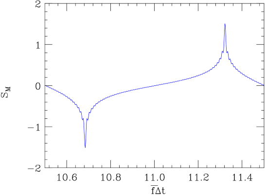
Figure 2: The sum wake at the last bunch in a train vs bunch spacing, due to a uniform distribution of mode frequencies (Eq. 4). The total frequency spread $\Delta_{\delta f}=5.8\%$, and $N_{c}=102$.

Suppose we add frequency errors to our model. We can do this by, in each term in the sum of Eq. 4, multiplying the frequency by the factor $(1+\delta f_{err}r_{n})$, with $\delta f_{err}$ the rms (relative) frequency error and $r_{n}$ a random number with rms 1. Doing this, considering a uniform distribution in frequency errors with rms $\delta f_{err}=10^{-4}$, Fig. 2 becomes Fig. 3. Note that this perturbation is small compared to the frequency spacing $5.7\times 10^{-4}$, so it does not really change the frequency distribution significantly. Nevertheless, because of resonance-like behavior we can see a large effect on $S_{M}$ throughout the range between the horns of Fig. 2 ($10.68\leq{\bar{f}}\Delta t\leq 11.32$). To model cell-to-cell misalignments, we multiply each term in the sum of Eq. 4 by the random factor $r_{n}$. The results, for a uniform distribution of errors with rms 1, are shown in Fig. 4. Again resonance-like behavior is seen throughout the range between the horns of Fig. 2.

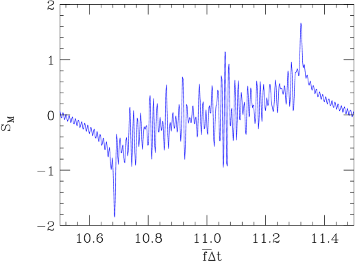
Figure 3: The sum wake at the last bunch in a train vs bunch spacing, due to a uniform distribution of frequencies, including frequency errors. The total frequency spread $\Delta_{\delta f}=5.8\%$, the number of modes $N_{c}=102$, and rms relative frequency error is $10^{-4}$.

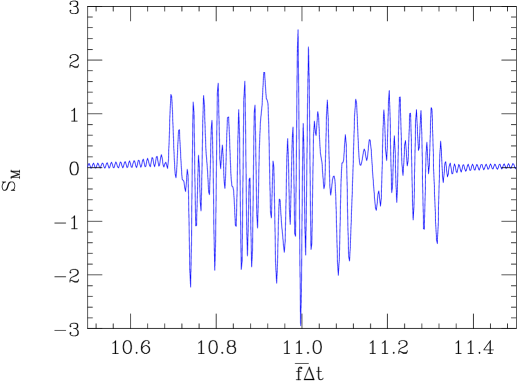
Figure 4: The sum wake at the last bunch in a train vs bunch spacing, due to a uniform distribution of frequencies, including random misalignment errors with rms 1. The total frequency spread $\Delta_{\delta f}=5.8\%$ and then number of modes $N_{c}=102$.

We can understand these results in the following manner: Only when there are no errors does using a uniform frequency distribution suppress the resonance in the region near the integer resonance. But otherwise, using a uniform frequency distribution basically only reduces the size of the resonances, at the expense of extending the range in bunch spacings where they can be excited. Instead of being localized in the region near the integer resonance (${\bar{f}}\Delta t\approx n$), resonance-like behavior can now be excited anywhere between the limits

$$({\bar{f}}\Delta t)_{\pm}={n\over 1\mp\Delta_{\delta f}/2}\quad.$$ (5)

Note that this implies that if $\Delta_{\delta f}>1/({\bar{f}}\Delta t)$, then the resonance-like behavior cannot be avoided no matter what bunch spacing (fractional part) is chosen. For example, for the X-band linac in the NLC, where the total width of the dipole frequency distribution (of the dominant first band modes) is 10%, even for the alternate (1.4 ns) bunch spacing, where the integer part of ${\bar{f}}\Delta t$ is 21, the resonance region cannot be avoided.

References

- [1] K. Bane and Z. Li, “Dipole Mode Detuning in the Injector Linacs of the NLC,” SLAC/LCC Note in preparation.
- [2] D. Schulte, presentation given in an NLC Linac meeting, summer 1999.
- [3] K. Bane and R. Gluckstern, Part. Accel., 42, 123 (1994).