Analytical Formula for Weak Multi-Bunch Beam Break-Up in a Linac

In designing linac structures for multi-bunch applications we are often interested in estimating the effect of relatively weak multi-bunch beam break-up (BBU), due to the somewhat complicated wakefields of detuned structures. This, for example, is the case for the injector linacs of the JLC/NLC linear collider project (see Ref. [1]). Deriving an analytical formula for such a problem is the subject of this report. Note that the more studied multi-bunch BBU problem, i.e. the effect on a bunch train of a single strong mode, the so-called “cumulative beam break-up instability” (see, e.g. Ref. [2]), is a somewhat different problem, and one for which the approach presented here is probably not very useful.

In Ref. [3] an analytical formula for single-bunch beam break-up in a smooth focusing linac, for the case without energy spread in the beam, is derived, the so-called Chao-Richter-Yao (CRY) model for beam break-up. Suppose the beam is initially offset from the accelerator axis. The beam break-up downstream is characterized by a strength parameter $\Upsilon(t,s)$, where $t$ represents position within the bunch, and $s$ position along the linac. When $\Upsilon(t,s)$ is small compared to 1, the growth in betatron amplitude in the linac is proportional to this parameter. When applied to the special case of a uniform longitudinal charge distribution, and a linearly growing wakefield, the result of the calculation becomes especially simple. In this case the growth in orbit amplitude is given as an asymptotic power series in $\Upsilon(t,s)$, and the series can be summed to give a closed form, asymptotic solution for single-bunch BBU. The derivation of an analytic formula for multi-bunch BBU is almost a trivial modification of the CRY formalism. We will here reproduce the important features of the single-bunch derivation of Ref. [3] (with slightly modified notation), and then show how it can be modified to obtain a result applicable to multi-bunch BBU.

Let us consider the case of single-bunch beam break-up, where a beam is initially offset by distance $y_{0}$ in a linac with acceleration and smooth focusing. We assume that there is no energy spread within the beam. The equation of motion is

$${1\over E(s)}{d\over ds}\left[E(s){dy(t,s)\over ds}\right]+{y(t,s)\over\beta^{2}(s)}={e^{2}N_{t}\over E(s)}\int_{-\infty}^{t}dt^{\prime}\,y(t^{\prime},s)\lambda_{t}(t^{\prime})W(t-t^{\prime})\ ,$$ (1)

with $y(t,s)$ the bunch offset, a function of position within the bunch $t$, and position along the linac $s$; with $E$ the beam energy, $[1/\beta(s)]$ the betatron wave number, $eN_{t}$ the total bunch charge, $\lambda_{t}(t)$ the longitudinal charge distribution, and $W(t)$ the short-range dipole wakefield. Our convention is that negative values of $t$ are toward the front of the bunch. Let us, for the moment, limit ourselves to the problem of no acceleration and $\beta$ a constant. A. Chao in Ref. [3] expands the solution to the equation of motion for this problem in a perturbation series

$$y(t,s)=\sum_{n=0}^{\infty}y^{(n)}(t,s)\quad,$$ (2)

with the first term given by free betatron oscillation [$y^{(0)}=y_{0}\cos(s/\beta)$]. He then shows that the solution for the higher terms at position $s=L$, after many betatron oscillations, is given by

$$y^{(n)}(t,L)\approx{y_{0}\over n!}\left({ie^{2}N_{t}L\beta\over 2E}\right)^{n}R_{n}(t)e^{iL/\beta}\quad,$$ (3)

with

$$R_{n}(t) = \int_{-\infty}^{t}dt_{1}\,\lambda(t_{1})W(t-t_{1})\int_{-\infty}^{t_{1}}dt_{2}\,\lambda(t_{2})W(t_{1}-t_{2})$$ (4)

$$\cdots\int_{-\infty}^{t_{n-1}}dt_{n}\,\lambda(t_{n})W(t_{n-1}-t_{n})\ ,$$

and $R_{0}(z)=1$. An observable $y$ is meant to be the real part of Eq. 2. The effects of adiabatic acceleration, i.e. sufficiently slow acceleration so that the energy doubling distance is large compared to the betatron wave length, and $\beta$ not constant, can be added by simply replacing $(\beta/E)$ in Eq. 3 by $\langle\beta/E\rangle$, where angle brackets indicate averaging along the linac from $s=0$ to $s=L$. For example, if the lattice is such that $\beta\sim E^{\zeta}$ then $\langle\beta/E\rangle=(\beta_{0}/E_{0})g(E_{f}/E_{0},\zeta)$, where subscripts “0” and “$f$” signify, respectively, initial and final parameters, and

$$g(x,\zeta)={1\over\zeta}\left({x^{\zeta}-1\over x-1}\right)\quad\quad\quad[{\beta\sim E^{\zeta}}].$$ (5)

Chao then shows that for certain simple combinations of bunch shape and wake function shape the integrals in Eq. 4 can be performed analytically, and the result becomes an asymptotic series in powers of a strength parameter. For example, for the case of a uniform charge distribution of length $\ell$ (with the front of the bunch at $t=0$), and a wake that varies as $W=W^{\prime}t$, the strength parameter is

$$\Upsilon(t,L)={e^{2}N_{t}LW^{\prime}t^{2}\beta_{0}\over 2E_{0}\ell}g(E_{f}/E_{0},\zeta)\quad.$$ (6)

If $\Upsilon$ is small compared to 1, the growth is well approximated by $\Upsilon$. If $\Upsilon$ is large, the sum over all terms can be performed to give a closed form, asymptotic expression.

For multi-bunch BBU we are mainly concerned with the interaction of the different bunches in the train, and will ignore wakefield forces within bunches. The derivation is nearly identical to that for the single-bunch BBU. However, in the equation of motion, Eq. 1, the independent variable $t$ is no longer a continuous variable, but rather $t$ takes on discrete values $t_{m}=m\Delta t$, where $m$ is a bunch index and $\Delta t$ is the bunch spacing. Also, $W$ now represents the long-range wakefield. Let us assume that there are $M$, equally populated bunches in a train; i.e. $N_{t}=MN$, with $N$ the particles per bunch. The solution is again expanded in a perturbation series. In the solution, Eq. 3, the $R_{n}(t)$, which are smooth functions of $t$, are replaced by

$${\cal R}_{m}^{(n)}={1\over M}\sum_{j=1}^{m-1}W[(m-j)\Delta t]{\cal R}_{j}^{(n-1)}\quad,$$ (7)

(with ${\cal R}_{j}^{0}=1$), which is a function of a discrete parameter, the bunch index $m$. Note that ${\cal R}_{m}^{(1)}=S_{m}/M$, with $S_{m}$ the sum wake.

Generally the sums in Eq. 7 cannot be given in closed form, and therefore a closed, asymptotic expression for multi-bunch BBU cannot be given. We can still, however, numerically compute the individual terms equivalent to Eq. 3 for the single bunch case. For example, the first order term in amplitude growth is given by

$$\Upsilon_{m}={e^{2}NLS_{m}\beta_{0}\over 2E_{0}}g(E_{f}/E_{0},\zeta)\quad\quad\quad[m=1,\ldots,M]\ .$$ (8)

If this term is small compared to 1 for all $m$, then BBU is well characterized by $\Upsilon$. If it is not small, though not extremely large, the next higher terms can be computed and their contribution added. For $\Upsilon$ very large, this approach may not be very useful.

From our derivation we see that there is nothing that fundamentally distinguishes our BBU solution from a single-bunch BBU solution. If we consider again the single-bunch calculation, for the case of a uniform charge distribution of length $\ell$, we see that we need to perform the integrations for $R_{n}$ in Eq. 4. If we do the integrations numerically, by dividing the integrals into discrete steps $t_{n}=(n-1)\Delta t$ and then performing quadrature by rectangular rule, we end up with Eq. 7 with $M=\ell/\Delta t$. The solution is the same as our multi-bunch solution. What distinguishes the multi-bunch from the single-bunch problem is that the wakefield for the multi-bunch case is not normally monotonic and does not vary smoothly with longitudinal position. For such a case it may be more difficult to decide how many terms are needed for the sum to converge.

In Fig. 1 we give a numerical example: the NLC prelinac with the optimized $3\pi/4$ S-band structure, but with $10^{-5}$ systematic frequency errors, with the nominal (2.8 ns) bunch spacing (see Ref. [1]). The diamonds give the first order (a) and the second order (b) perturbation terms. The crosses in (a) give the results of a smooth focusing simulation program (taking $\beta\sim E^{1/2}$), where the free betatron term has been removed. We see that the agreement is very good; i.e. the first order term is a good approximation to the simulation results. In (b) we note that the next order term is much smaller.

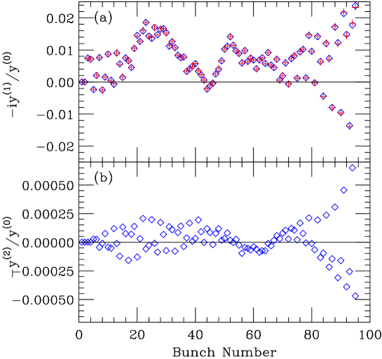
Figure 1: A numerical example: the NLC prelinac with the optimized $3\pi/4$ S-band structure, but with $10^{-5}$ systematic frequency errors, with the nominal (2.8 ns) bunch spacing (see Ref. [1]). Here $N=1.2\times 10^{10}$, $E_{0}=1.98$ GeV, $E_{f}=10.$ GeV, $L=558$ m; the rms of the sum wake $S_{rms}=.005$ MV/nC/m². The diamonds give the first order (a) and the second order (b) perturbation terms. The crosses in (a) give smooth focusing simulation results with the free betatron term removed.

References

- [1] K. Bane and Z. Li, “Dipole Mode Detuning in the Injector Linacs of the NLC,” SLAC/LCC Note in preparation.
- [2] R. Helm and G. Loew, Linear Accelerators, North Holland, Amsterdam, 1970, Chapter B.1.4.
- [3] A. Chao, “Physics of Collective Instabilities in High-Energy Accelerators”, John Wiley & Sons, New York (1993).