Path Integral Monte Carlo Simulation of the Low-Density Hydrogen Plasma

Abstract

Restricted path integral Monte Carlo simulations are used to calculate the equilibrium properties of hydrogen in the density and temperature range of $9.83\times 10^{-4}\rm\leq\rho\leq 0.153\,\rm gcm^{-3}$ and $5000\leq T\leq 250\,000\,\rm K$. We test the accuracy of the pair density matrix and analyze the dependence on the system size, on the time step of the path integral and on the type of nodal surface. We calculate the equation of state and compare with other models for hydrogen valid in this regime. Further, we characterize the state of hydrogen and describe the changes from a plasma to an atomic and molecular liquid by analyzing the pair correlation functions and estimating the number of atoms and molecules present.

I Introduction

In spite of the simple composition, hydrogen exhibits a surprisingly complex phase diagram, which is the subject of numerous experimental and theoretical approaches. In this work, we study the high temperature regime of $5000\leq T\leq 250\,000\,\rm K$ where hydrogen undergoes a smooth transition with increasing temperature from a molecular fluid through an atomic regime and finally to a two component plasma of electrons and protons (see Fig. 1). The properties of hydrogen in this regime are crucial for the evolution of stars and the characteristics of the Jovian planets.

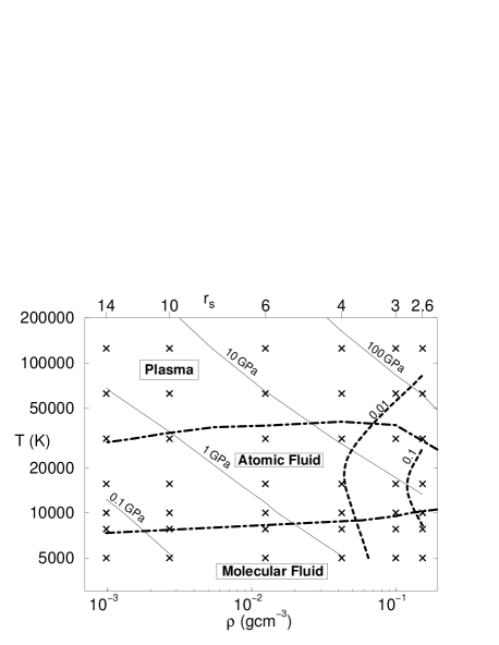
Figure 1: Phase diagram of hydrogen as a function of temperature and density for the different regimes: plasma, the atomic and the molecular regime. The dash-dot lines indicate the approximate boundaries. The crosses indicate the parameters for which PIMC simulations have been performed, the solid lines are isobars, and the dashed lines represent contour lines of constant permutation probability of the electrons (as indicated on the line.)

A variety of simulation techniques and analytical models have been developed to describe hydrogen at low density. This regime has been studied with chemical models SC92 ; ER85b ; Ki97 that describe hydrogen as a mixture of interacting molecules, atoms, free protons and electrons. The chemical composition is determined by minimizing an approximate free energy function constructed from known theoretical limits. In this paper, we focus on low and intermediate densities $9.83\times 10^{-4}\rm\leq\rho\leq 0.153\,\rm gcm^{-3}$ corresponding to $14\geq r_{s}\geq 2.6$, where one expects the chemical models to work well although the properties of hydrogen are determined by the complex interplay of long-range Coulomb forces leading to strong coupling and bound states as well as degeneracy effects.

All these effects can also be described from first principles simulation. There are ab initio methods such as restricted path integral Monte Carlo simulations (PIMC) PC94 ; Ma96 ; Mi99 and density functional theory molecular dynamics (DFT-MD) Le00 ; Ga99 . The focus of the work is to test the equation of state (EOS) derived from chemical models and the actual density-temperature limits of the validity of the chemical picture. Additionally, we provide data to determine the parameters of the free energy models. Chemical models are expected to become inaccurate in regions of high density where the lifetime of molecules reduces to a few molecular vibrations Ga99 .

We present results from new, more accurate, PIMC simulations. First, we analyze the accuracy of the pair density matrix and the error of the “time” discretization. Then we analyze the finite size dependence of the derived EOS and discuss the fixed node errors by comparing results from simulations using free particle (FP) nodes and variational nodes. Furthermore, we calculate pair correlation functions which we use in conjunction with a cluster analysis to characterize the state of hydrogen at different temperatures and densities. We use atomic units (lengths in Bohr radii and energies in Hartrees) throughout this work except where indicated otherwise.

II Path Integral Monte Carlo Method

II.1 Restricted Path Integral

The density matrix (DM) of a fermion system at temperature $k_{B}T=1/\beta$ can be written as an integral over all paths ${\bf R}_{t}$,

$$\rho({\bf R}_{0},{\bf R}_{\beta};\beta)=\frac{1}{N!}\sum_{\mathcal{P}}\>(-1)^{\mathcal{P}}\!\!\!\!\!\oint\limits_{{\bf R}_{0}\rightarrow{\mathcal{P}}{\bf R}_{\beta}}\!\!\!\!\!\!d{\bf R}_{t}\;\;e^{-S[{\bf R}_{t}]}.$$ (1)

${\bf R}_{t}$ stands for the entire paths of $N$ particles in $3$ dimensional space ${\bf R}_{t}=({\bf r}_{1t},\ldots,{\bf r}_{Nt})$ beginning at ${\bf R}_{0}$ and ending at ${\mathcal{P}}{\bf R}_{\beta}$. ${\mathcal{P}}$ labels the permutation of the particles and $(-1)^{\mathcal{P}}$ to its signature. For non-relativistic particles interacting with a potential $V({\bf R})$, the action of the path $S[{\bf R}_{t}]$ is given by,

$$S[{\bf R}_{t}]=\int_{0}^{\beta}\!dt\left[\frac{m}{2}\left|\frac{d{\bf R}(t)}{\hbar dt}\right|^{2}+V({\bf R}(t))\right]+\mbox{const}.$$ (2)

In practice one discretizes Ce95 the path into a finite number of imaginary time slices $M$ corresponding to a time step $\tau=\beta/M$.

For fermionic systems the integration is complicated due to the cancellation of positive and negative contributions to the integral, (the fermion sign problem). It has been shown Ce91 ; Ce96 that one can evaluate the path integral by restricting the path to only specific positive contributions. One introduces a reference point ${\bf R}^{*}$ on the path that specifies the nodes of the DM, $\rho({\bf R},{\bf R}^{*},t)=0$. A node-avoiding path for $0<t\leq\beta$ neither touches nor crosses a node: $\rho({\bf R}(t),{\bf R}^{*},t)\not=0$. By restricting the integral to node-avoiding paths,

$$\rho_{F}({\bf R}_{\beta},{\bf R}^{*};\beta) =$$

$$\int\!\!d{\bf R}_{0}\> \rho_{F} ({\bf R}_{0},{\bf R}^{*};0)\!\!\!\!\!\!\!\!\!\!\!\oint\limits_{{\bf R}_{0}\rightarrow{\bf R}_{\beta}\in\Upsilon({\bf R}^{*})}\!\!\!\!\!\!\!\!\!\!\!\!\!d{\bf R}_{t}\;\;e^{-S[{\bf R}_{t}]},$$ (3)

($\Upsilon({\bf R}^{*})$ denotes the restriction) the contributions are positive and therefore PIMC represents, in principle, a solution to the sign problem. The method is exact if the exact fermionic DM is used for the restriction. However, the exact DM is only known in a few cases. Most applications have approximated the fermionic DM by a determinant of single particle DMs,

$$\rho({\bf R},{\bf R^{\prime}};\beta)=\left|\begin{array}[]{ccc}\rho_{1}({\bf r}_{1},{\bf r}^{\prime}_{1};\beta)&\ldots&\rho_{1}({\bf r}_{N},{\bf r}^{\prime}_{1};\beta)\\ \ldots&\ldots&\ldots\\ \rho_{1}({\bf r}_{1},{\bf r}^{\prime}_{N};\beta)&\ldots&\rho_{1}({\bf r}_{N},{\bf r}^{\prime}_{N};\beta)\end{array}\right|\quad.$$ (4)

This approach has been extensively applied using the free particle (FP) nodes derived from the single-particle density matrix Ce96 :

$$\rho_{1}({\bf r},{\bf r}^{\prime},\beta)=(4\pi\lambda\beta)^{-3/2}\>\mbox{exp}\left\{-({\bf r}-{\bf r}^{\prime})^{2}/4\lambda\beta\right\}$$ (5)

with $\lambda=\hbar^{2}/2m$, including applications to dense hydrogen PC94 ; Ma96 ; Mi99 . It can be shown that for temperatures larger than the Fermi energy, the interacting nodal surface approaches the FP nodal surface. In addition, in the limit of low density, exchange effects are negligible: the nodal constraint has a small effect on the path and therefore its precise shape is not important. The FP nodes also become exact in the limit of high density when kinetic effects dominate over the interaction potential. However, for the densities and temperatures under consideration, interactions could have a significant effect on the nodal surfaces.

To gain some quantitative estimate of the possible effect of the nodal restriction on the thermodynamic properties, it is necessary to try an alternative. In addition to FP nodes, we used nodal surface of a variational density matrix (VDM) MP00 derived from a variational principle that includes interactions and atomic and molecular bound states. We assume a trial DM with parameters $q_{i}$ that depend on imaginary time $\beta$ and ${\bf R^{\prime}}$,

$$\rho({\bf R},{\bf R^{\prime}};\beta)=\rho({\bf R},q_{1},\ldots,q_{m})\;.$$ (6)

By minimizing the integral:

$$\int\!d{\bf R}\left(\frac{\partial\rho({\bf R},{\bf R^{\prime}};\beta)}{\partial\beta}+{\mathcal{H}}\,\rho({\bf R},{\bf R^{\prime}};\beta)\right)^{\!\!2}=0\quad,$$ (7)

one determines equations for the dynamics of the parameters in imaginary time:

$$\frac{1}{2}\frac{\partial H}{\partial\vec{q}}\;+\;\,\stackrel{{\scriptstyle{\textstyle\leftrightarrow}}}{{{\mathcal{N}}}}\>\dot{\vec{q}}=0\;\;\;\;\mbox{where}\;\;\;\;H\equiv\int\rho{\mathcal{H}}\rho\;d{\bf R}\;.$$ (8)

The norm matrix is:

$${\mathcal{N}}_{ij} = \lim_{q^{\prime}\rightarrow q}\frac{\partial^{\,2}}{\partial q_{i}\partial q^{\prime}_{j}}\left[\int\!d{\bf R}\;\rho({\bf R},\vec{q}\,;\beta)\;\rho({\bf R},\vec{q}\>^{\prime}\,;\beta)\right]\;.$$ (9)

We assume the DM is a Slater determinant of single particle Gaussian functions

$$\rho_{1}({\bf r},{\bf r}^{\prime},\beta)=(\pi w)^{-3/2}\>\mbox{exp}\left\{-({\bf r}-{\bf m})^{2}/w+d\right\}$$ (10)

where the variational parameters are the mean ${\bf m}$, squared width $w$ and amplitude $d$. The differential equations for this ansatz are given in MP00 . The initial conditions at $\beta\longrightarrow 0$ are $w=2\beta$, ${\bf m}={\bf r}^{\prime}$ and $d=0$ in order to regain the correct FP limit. It follows from Eq. 7 that at low temperature, the VDM goes to the lowest energy wave function within the variational basis. For an isolated atom or molecule this will be a bound state, in contrast to the delocalized state of the FP DM. A further discussion of the VDM properties is given in MP00 . Note that these nodes are only used to determine the nodal restriction in Eq. (II.3). The complete potential is taken into account in the path integral action as discussed in detail in Ce95 .

II.2 Accuracy of the Method

The numerical implementation of the PIMC method requires one to make several approximations. Inaccuracies can be caused by statistical errors from the MC integration, inaccuracies in the numerically determined pair density matrices, a dependence on the time step of the path integral because of $N$-body ($N\geq 3$) correlations, finite size effects, and nodal errors from approximations in the trial density matrix. Their effects on the accuracy of the computed thermodynamic averages are quantitatively estimated in this section.

Statistical errors in the estimators for the thermodynamic quantities are calculated from the block averages generated by the MC simulations. The correlations between blocks are taken into account by performing a blocking analysis AT87 . The resulting error bars (one standard deviation) are given for all observables throughout this paper as a number in parenthesis referring to the least significant digit.

In the following discussion, we compare the internal energy and the pressure calculated using the virial theorem:

$$3Pv=2K+V$$ (11)

where $v$ is the volume of the simulation cell, $K$ the kinetic energy and $V$ the potential energy. Accurate estimation of the pressure requires a high accuracy in the kinetic and the potential energies because they tend to cancel out. In the molecular regime at low density, both terms, dominated by intra-molecular contributions, cancel to a large extent leaving behind the molecular gas pressure, which is much less than the inter-molecular forces. As a result, the pressure is, in general, significantly more sensitive to approximations than other quantities such as the internal energy.

II.2.1 Pair Density Matrix

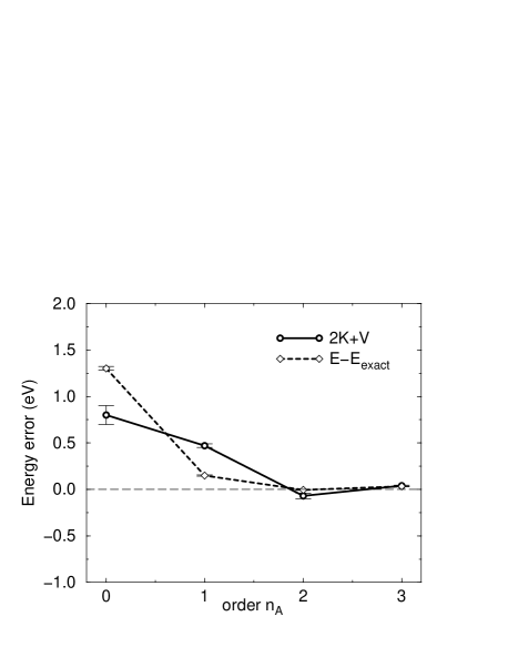
Figure 2: Accuracy study of PIMC simulations of the isolated hydrogen atom using different orders $n_{\rm A}$ in the expansion formula 12 for the action and energy. The calculated $2K+V$ (exact value equals zero) and the deviation from the exact potential energy of $-27.2\,\rm eV$ are shown for different orders from simulations at $T=10\,000\,\rm K$ using $\tau^{-1}=10^{6}\rm K$.

If one only used the bare potential as in Eq. 2 (the primitive approximation for the action), the convergence would be very slow BM00 and would result in an extremely inefficient many-particle simulations. Instead, we numerically solve the two-particle problem with the matrix squaring technique St68 . Numerical representations of the exact pair density matrices are stored in tables used by the PIMC simulation program by expanding in the small variables $s$ and $z$:

$$u({\bf r},{\bf r}^{\prime};\tau)=\frac{1}{2} \left[u_{0}(r;\tau)+u_{0}(r^{\prime};\tau)\right]$$ (12)

$$+\sum_{k=1}^{n_{\rm A}}\sum_{j=0}^{k}u_{kj}(q;\tau)\,z^{2j}\,s^{2(k-j)},$$

where

$$q=\frac{1}{2}(|{\bf r}|+|{\bf r}^{\prime}|)\quad s=|{\bf r}-{\bf r}^{\prime}|\quad z=|{\bf r}|-|{\bf r}^{\prime}|\quad,$$ (13)

and ${\bf r}$ and ${\bf r}^{\prime}$ denote the separation of the two particles at adjacent time slices. The accuracy of these tables is crucial for all computed results. Using the precomputed pair density matrices allows one to employ a much larger time step because one starts with a solution of the two-particle problem. Fig. 2 shows how accurate this method is. The internal energy of an isolated hydrogen atom at sufficiently low temperature ($T=10\,000\,\rm K$) in a large box ($L=26$) is compared with the exact ground state energy of $-13.6\,\rm eV$. The temperature was chosen low enough so that excited states can be neglected; the contribution to the energy from the occupation of the first excited state is $7\cdot 10^{-5}\,\rm eV$ at this temperature. Also shown is how well the kinetic energy $K$ and the potential energy $V$ satisfy the virial theorem $2K+V=0$, thus determining the accuracy with which the pressure can be determined. For a time step of $\tau^{-1}=10^{6}\rm K$, the analysis shows a quick convergence with the order of terms considered in the action expansion Eq. (12). Using terms up $n_{\rm A}=3$ reduces the error to $0.033\,(3)\,\rm eV$ in energy and to $0.039\,(8)\,\rm eV$ for $2K+V$. This corresponds to an inaccuracy in the pressure equivalent to a non-interacting molecular gas at $T=260\,(30)\,\rm K$.

II.2.2 Time step dependence

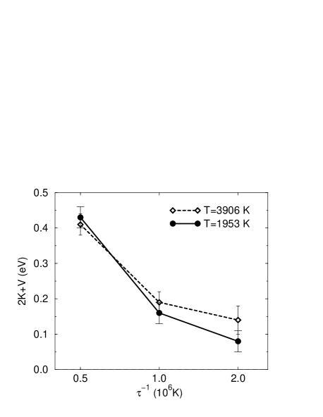
Figure 3: The error in the virial as a function of the number of time slices for an isolated hydrogen molecule. The classical nuclei are fixed at the equilibrium bond length, thus the exact value for $2K+V$ is zero at a sufficiently low temperature.

Employing the pair approximation of the density matrix does not include correlation effects for three or more particles (for example between one electron and two protons). We now estimate how small the time step must be to obtain a given accuracy for an isolated molecule. Fig. 3 shows results for different time steps and temperatures with the nuclei kept fixed at the equilibrium position of $R=1.4008$. From the virial theorem, it follows that $2K+V=0$ at a sufficiently low temperature. The exact energy per atom is $-15.973\rm\,eV$ KW64 . The $T$ dependence is small suggesting that the electrons are in the ground state. However, one finds a significant dependence on the time step. Using $\tau^{-1}=2\times 10^{6}\rm K$ reduces the error in the energy per atom to $0.036(3)\,\rm\,eV$ and in $2K+V$ to $0.090\,(16)\,\rm eV$. The time step error is larger than the errors of the inaccuracies in the pair density matrices discussed above. The error in $2K+V$ corresponds to a pressure of an non-interacting molecular gas at $T=700\,(100)\,\rm K$, which provides us with an approximate limit of accuracy in the equation of state calculated from many-particle simulations with $\tau^{-1}=2\times 10^{6}\rm K$.

II.2.3 Finite Size Dependence

The estimation of the finite size errors is more difficult to assess because the needed PIMC simulations are computationally much more demanding. The required computer time increases rapidly with the number of particles making it challenging to obtain converged results for paths corresponding to large systems.

Most results from many-body simulations reported in this work were calculated with $N=32$ pairs of electrons and protons in a periodically repeated simulation cell. To study the effect on $N$, we performed simulations for $N=16$ and $64$ pairs of protons and electrons for a density of $r_{s}=2.6$ and $T\geq 10\,000\,\rm K$. We chose the highest density under consideration because one expects the finite size dependence to be largest there due to the stronger interaction between the atoms.

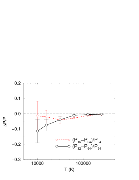
Figure 4: Finite size error of the pressure as a function of temperature relative to simulations with $N=64$ pairs of protons and electrons at a density of $r_{s}=2.6$.

The finite size dependence of the pressure, shown in Fig. 4, is small at high temperatures but grows to approximately $4\,(2)\,\%$ near $T=30\,000\,\rm K$. In this regime, the hydrogen undergoes structural changes involving the formation of atoms, which affect the pressure. This study provides us only with an estimate of the finite size dependence. An extrapolation to $N\to\infty$ would require significantly larger systems, not currently feasible at low temperatures.

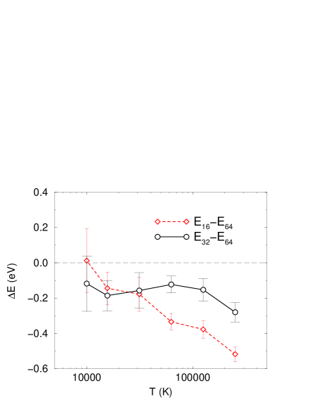
Figure 5: Finite size error of the internal energy as a function of temperature relative to simulations with $N=64$ pairs of particles at a density of $r_{s}=2.6$.

Fig. 5 shows the finite size error of the internal energy. The smaller systems are more strongly bound by approximately $0.2~{}\rm eV$ per atom, probably because of the interaction of a charge with its own image. For lower densities, we expect this value to be smaller.

II.2.4 Nodal Approximation

In the above, we have studied controlled approximations. The only uncontrolled approximation in the restricted PIMC method is the use of trial density matrix to constrain the paths. The nodal surfaces are important only if the electrons are degenerate: at low temperatures or at high densities. Recall that in this work we focus on hydrogen only at low density, where the electrons are bound in atoms and molecules and have a low or moderate degeneracy. Even at low density, one still needs a nodal surface in order to prevent the formation of unphysical clusters like $H_{3}$ and $H_{4}$ or even the collapse of the entire system, but the precise shape of the nodes is not important at low density as shown in Fig. 6.

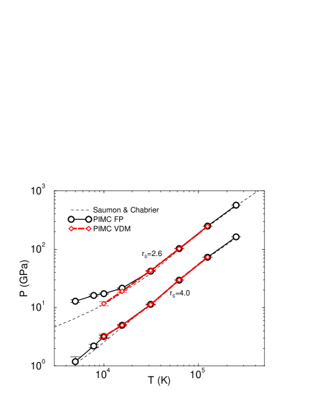
Figure 6: The effect on the pressure of two different nodal surfaces: of the free particle density matrix and of the variational density matrix.

Comparing FP and VDM nodes for $r_{s}=2.6$, one only finds differences in the pressure for $T\leq 15\,625\,\rm K$, which is approximately where, at this density, the system shows a significant molecular signature (see section III.2 and Fig. 16). In this regime, FP nodes systematically lead to a too high pressure, while simulations with VDM nodes stay closer to the prediction of a semi-empirical chemical model SC92 . At a lower density, $r_{s}=4$, results from FP and VDM nodes agree within the error bars.

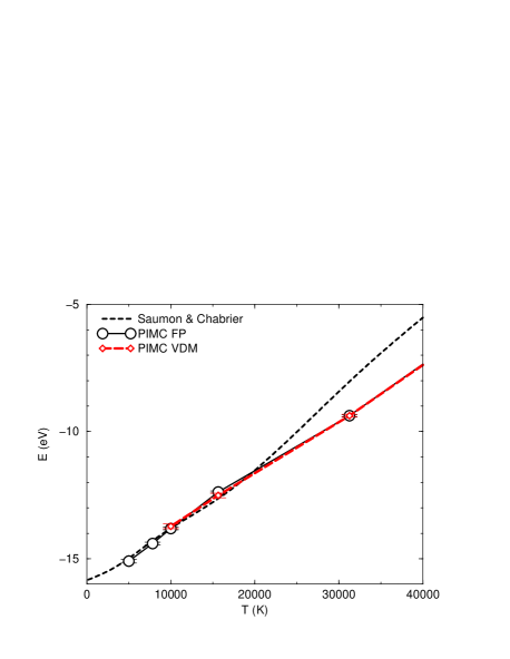
Figure 7: Internal energy computed with PIMC using two different nodal surfaces: the free particle density matrix and the variational density matrix.

The differences in the internal energy, as shown in Fig. 7, using FP and VDM nodes are significantly smaller than the pressure deviations. One either finds agreement within the error bars or that VDM nodes predict lower internal energies, which was used in MC00 to show that VDM nodes are the more accurate nodal surface. The observed energy differences did not exceed $0.1\,\rm eV$ per atom.

For even lower density, the nodes are less relevant because they become only important in a collision of two molecules, which occur less frequently at lower density. This trend can also be understood in terms of the degeneracy of the electrons. The degree of degeneracy manifests itself in the path integral formalism by the probability for the electrons to be involved in a permutation. At high temperature, the paths are very short and permutations are rare. At low temperature and high density, the paths are long and can form long permutation cycles. However in hydrogen at low density, the paths are localized due to the attraction in atoms and molecules and permutations are rare. Fig. 1 shows that the permutation probability never reaches $1\%$ for $r_{s}=4$ (see Tab. 1). For higher densities, the permutation probability is increased as indicated by the contour lines. This is consistent with the temperature and density dependence of the nodal error in pressure and internal energy discussed above.

III Results

III.1 Equation of State

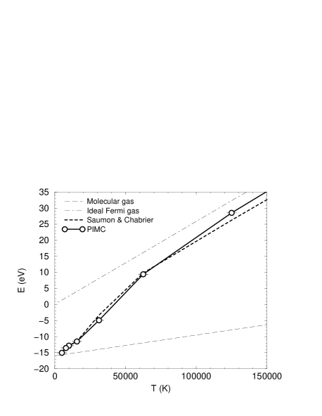
Figure 8: Internal energy per atom vs. temperature for a density of $r_{s}=10$ comparing the SC-EOS SC92 with PIMC calculations.

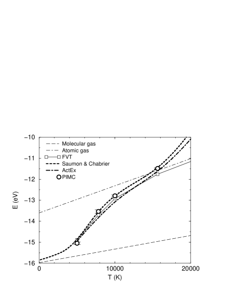
Figure 9: Internal energy per atom vs. temperature for a density of $r_{s}=10$ as shown in Fig. 8 but here for lower temperatures also including results from the activity expansion Ro90 .

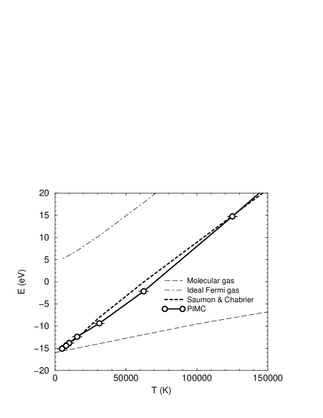
Figure 10: Internal energy per atom vs. temperature as shown in Fig. 8 but here for a density of $r_{s}=2.6$.

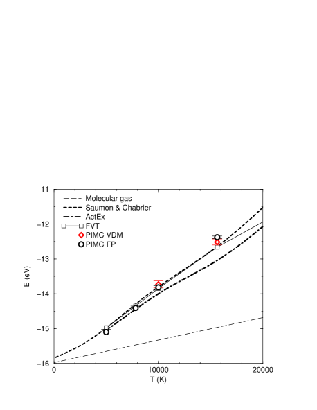
Figure 11: Internal energy per atom vs. temperature for a density of $r_{s}=2.6$ as shown in Fig. 10 but here for lower temperatures also including results from the activity expansion (ActEx) Ro90 and the fluid variational theory (FVT) Ju00 .

Tab. 1 gives the complete set of energies and pressures at 6 densities and 8 temperatures. We now compare these results with several models for hydrogen. We begin our discussion by studying the internal energy per atom as a function of temperature shown in Figs. 8 - 11 for two selected densities corresponding to $r_{s}=10.0$ and $2.6$. Generally, we find a fairly good overall agreement with the EOS by SC SC92 over the entire temperature and density range discussed in this work. The agreement is particularly good in the molecular and atomic regime for $r_{s}=10.0$, as shown in Fig. 9. There the SC energies are within the error bars of the PIMC results. At higher temperature shown in Fig. 8, we find systematic deviations of up to 5 eV per atom at $T=250\,000\,\rm K$. They indicate that the SC energies are too low at high temperatures and too high at intermediate temperatures (see Fig. 8). One possible explanation for the deviations at high temperature is that the SC model underestimates the degree of ionization (see discussion in Sc95 ).

We also studied these deviations as a function of density. The cross-over temperature, above which the SC-EOS underestimates the energy, increases with density. At $r_{s}=10.0$, the cross-over is near $70\,000\,\rm K$ compared to $130\,000\,\rm K$ (Fig. 10) at $r_{s}=2.6$. At temperatures below $20\,000\,\rm K$ for $r_{s}=2.6$, one also finds some small deviations up to $0.5\,\rm eV$ per atom (Fig. 11).

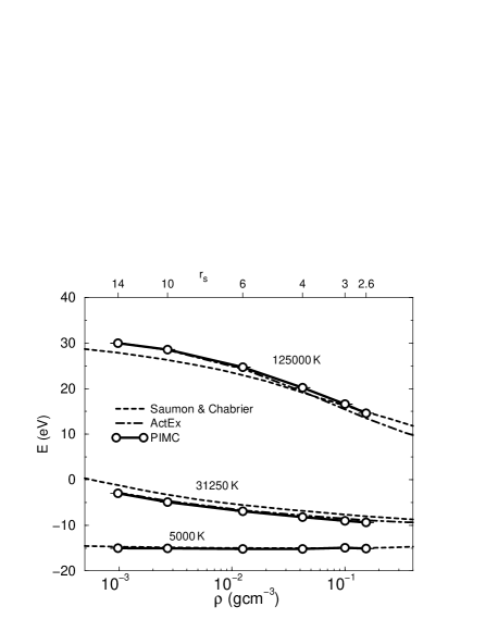
Figure 12: Internal energy per atom vs. density for different temperatures from SC-EOS SC92 , the activity expansion (ActEx) Ro90 (not shown for $5000\,\rm{K}$ since nearly identical to SC) and PIMC calculations .

Fig. 12 shows a comparison of energy vs. density for several temperatures. It shows that the SC-EOS overestimates the energy for $T=5000\,\rm K$ and $31\,250\,\rm K$ and underestimates it for $125\,000\,\rm K$ for densities higher than those corresponding to $r_{s}=2.6$.

Now let us compare the pressure from the SC-EOS with that from the PIMC simulation using Eq. 11 in Tab. 1.

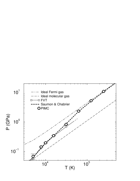
Figure 13: Pressure vs. temperature at a density of $r_{s}=10$ showing results from the fluid variational theory Ju00 , the SC-EOS SC92 , and PIMC simulations.

We find remarkably good agreement of the entire range of temperature and density under consideration. For a low density such as $r_{s}=10.0$, this is shown in Fig. 13. As expected, one finds that both methods interpolate between the limit of an ideal Fermi gas at high temperatures and non-interacting molecular gas at low temperatures. Fig. 14 confirms the good agreement at a higher density of $r_{s}=2.6$. As a result of the strong interactions at this density, one finds that the pressure at low temperatures is significantly above the non-interacting molecular gas limit.

We find that the SC-EOS underestimates the pressure by about 3% for $T>62\,500\,\rm K$. This difference is outside the error bar from the approximations in PIMC discussed in section II.2 and could be interpreted as a further indication, in addition to the observed energy deviations, that the SC model underestimates the degree of ionization at high temperatures. For intermediate temperatures $62\,500\geq T\geq 15\,625\,\rm K$, one finds pressure differences, which are of the same magnitude as the finite size effects in PIMC. For temperatures below $15\,625\,\rm K$, the increased statistical errors in the PIMC pressure are of the same size as the observed deviations.

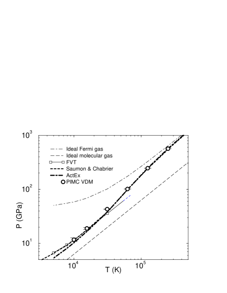
Figure 14: Pressure vs. temperature at a density of $r_{s}=2.6$ as shown in Fig. 13.

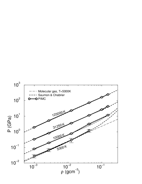
Figure 15: Pressure vs. density for different temperatures.

In Fig. 15. we show the pressure as a function of density, which confirms the good agreement. The figure also indicates that, at $5000\,\rm K$ and $r_{s}\geq 4$, the pressure is close to the pressure of a non-interacting molecular gas.

Table 1: Pressure and internal energy per atom and the resulting Hugoniot from PIMC simulations with $32$ pairs of particles and $\tau^{-1}=2\cdot 10^{6}\,\rm{K}$ using free particle nodes except for ^∗ where VDM nodes were employed instead. The probabilities $x$ for finding a proton in a given state for the three dominant species are derived from a cluster analysis. $P_{\rm perm}$ is the permutation probability for the electrons.

$r_{s}$	$T({\rm K})$	$P\,(\rm{GPa})~{}~{}~{}$	$E\,(\rm{eV})~{}~{}~{}$	$x_{\rm H^{+}}$	$x_{\rm H}$	$x_{\rm H_{2}}$	$P_{\rm perm}$
14.0	250 000	4.000 (2)	62.93 (4)				0.000
14.0	125 000	1.955 (2)	29.97 (4)	0.99	0.01	0.00	0.000
14.0	62 500	0.901 (2)	11.85 (4)	0.95	0.05	0.00	0.000
14.0	31 250	0.334 (2)	–2.97 (3)	0.64	0.36	0.00	0.000
14.0	15 625	0.127 (2)	–11.30 (4)	0.24	0.76	0.00	0.000
14.0	10 000	0.081 (4)	–12.43 (6)	0.12	0.72	0.15	0.000
14.0	7 812	0.047 (5)	–13.34 (13)	0.08	0.58	0.33	0.000
14.0	5 000	0.028 (6)	–15.00 (12)	0.01	0.11	0.88	0.000
10.0	250 000	10.902 (4)	62.00 (3)				0.000
10.0	125 000	5.259 (6)	28.56 (3)	0.98	0.02	0.00	0.000
10.0	62 500	2.329 (5)	9.41 (3)	0.90	0.10	0.00	0.000
10.0	31 250	0.831 (5)	–4.91 (3)	0.57	0.43	0.00	0.000
10.0	15 625	0.344 (4)	–11.49 (3)	0.23	0.74	0.02	0.000
10.0	10 000	0.198 (9)	–12.79 (5)	0.11	0.60	0.27	0.000
10.0	7 812	0.144 (7)	–13.54 (9)	0.03	0.34	0.62	0.000
10.0	5 000	0.068 (15)	–15.05 (7)	0.00	0.07	0.92	0.000
6.0	250 000	49.46 (3)	59.33 (4)				0.000
6.0	125 000	23.00 (3)	24.70 (4)	0.94	0.06	0.00	0.000
6.0	62 500	9.56 (2)	4.79 (3)	0.80	0.20	0.00	0.000
6.0	31 250	3.58 (3)	–6.92 (4)	0.52	0.46	0.01	0.000
6.0	15 625	1.52 (2)	–11.83 (4)	0.21	0.68	0.09	0.001
6.0	10 000	0.77 (4)	–13.38 (6)	0.08	0.49	0.40	0.000
6.0	7 812	0.63 (5)	–13.95 (7)	0.04	0.38	0.56	0.000
6.0	5 000	0.29 (9)	–15.17 (12)	0.00	0.09	0.90	0.000
4.0	250 000	162.46 (10)	55.63 (4)				0.000
4.0	125 000	73.00 (23)∗	20.24 (9)${}^{*}\;\;$	0.88	0.12	0.00	0.000
4.0	62 500	29.75 (16)∗	1.23 (6)${}^{*}\;\;$	0.72	0.26	0.00	0.001
4.0	31 250	11.22 (22)∗	–8.32 (8)${}^{*}\;\;$	0.47	0.46	0.03	0.004
4.0	15 625	5.01 (17)∗	–11.87 (6)${}^{*}\;\;$	0.19	0.58	0.18	0.008
4.0	10 000	3.23 (30)∗	–13.43 (11)∗	0.03	0.30	0.63	0.005
4.0	7 812	2.20 (14)	–14.29 (6)	0.01	0.18	0.80	0.004
4.0	5 000	1.19 (25)	–15.20 (9)	0.00	0.11	0.88	0.002
3.0	250 000	374.47 (14)	51.79 (2)				0.000
3.0	125 000	165.21 (22)	16.58 (4)	0.83	0.15	0.01	0.001
3.0	62 500	67.70 (25)	–1.04 (4)	0.66	0.29	0.01	0.005
3.0	31 250	26.67 (24)	–9.02 (4)	0.45	0.43	0.06	0.028
3.0	15 625	13.08 (28)	–12.29 (4)	0.15	0.42	0.34	0.059
3.0	10 000	9.26 (26)	–13.79 (4)	0.03	0.35	0.60	0.037
2.6	250 000	566.4 (4)	49.58 (4)				0.000
2.6	125 000	246.0 (5)∗	14.57 (5)${}^{*}\;\;$	0.80	0.17	0.01	0.002
2.6	62 500	101.7 (4)∗	–2.25 (4)${}^{*}\;\;$	0.65	0.28	0.02	0.014
2.6	31 250	43.1 (5)∗	–9.38 (5)${}^{*}\;\;$	0.42	0.38	0.09	0.078
2.6	15 625	19.0 (8)∗	–12.51 (9)${}^{*}\;\;$	0.14	0.42	0.33	0.168
2.6	10 000	11.7 (9)∗	–13.73 (10)∗	0.02	0.34	0.60	0.126

In our comparison, we also included results from the activity expansion by Rogers Ro90 , which shows very good agreement in pressure and internal energy (see Figs. 9, 11, and 12). The differences are small but increase with density. In the molecular and atomic regime, one also finds good agreement with the fluid variational theory (FVT) by Juranek and Redmer Ju00 as shown in Figs. 9, 11, 13, and 14. For higher temperatures, the FVT model is not applicable since it does not include ionization of atoms.

III.2 Pair Correlation Functions

There are four different pair correlation functions which can be directly obtained from many-body simulations and provide direct information about the state of the system. Shown in the following figures is an extensive set of pair correlations which allow one to estimate the microscopic structure of the system and allow a direct comparison with other simulations. The proton-proton pair correlation functions from PIMC simulations with free particle nodes are shown in Fig. 16. For $T\stackrel{{\scriptstyle\scriptstyle<}}{{\scriptscriptstyle\sim}}\>20\,000\,\rm K$ a peak at the bond length of $1.4$ emerges, which clearly demonstrates the formation of molecules. We found it useful to multiply the pair correlation function by an extra density factor $n=N/v$ so that the area under the peak is proportional to the molecular fraction. The peak height gets smaller with decreasing density as a result of entropic dissociation of the molecules, driven by the number of unbound states at low density. Thermal dissociation also reduces the number of molecules with increasing temperature. For $r_{s}\stackrel{{\scriptstyle\scriptstyle<}}{{\scriptscriptstyle\sim}}\>2$, we expect that pressure dissociation diminishes the number of molecules with increasing density BM00 but this density range is beyond the scope of this paper.

Figure 16: Proton-proton pair correlation function multiplied by the density $n$. The columns correspond to to $r_{s}$ values and the rows to different temperatures $T$.

The proton-electron pair correlation function multiplied by the density is shown in Fig. 17. The peak near the origin shows the increased probability of finding an electron near a proton due to the Coulomb attraction. The peak height decreases with temperature and increases with density because of thermal ionization and entropy ionization respectively. At low temperature, the peak can be interpreted as occupation of bound states although (unbound) scattering states can also contribute. From proton-electron pair correlation alone, one cannot distinguish between an atomic and a molecular state.

Figure 17: Proton-electron pair correlation function multiplied by the density $n$. The columns correspond to different $r_{s}$ values and the rows to different temperatures $T$.

Figs. 18 and 19 show the electron-electron pair correlation functions for pairs with anti-parallel spin. The peak at small separations comes from the formation of the molecular bond. For pairs of electrons with parallel spin, one always finds a strong repulsion due to the Pauli exclusion principle and to a lesser extent to the Coulomb repulsion. This is shown in Fig. 19.

Figure 18: Electron-electron pair correlation function for electrons with opposite spin multiplied by the density $n$ is shown. The columns correspond to different $r_{s}$ values and the rows to different temperatures $T$.

Figure 19: Electron-electron pair correlation function. The solid lines correspond to pairs of electrons with parallel spin. For the sake of comparison, we also show the pair correlation functions of pairs with opposite spin as dashed lines. This function is strongly peaked near the origin in the presence of molecules as shown in Fig. 18. The columns correspond to different $r_{s}$ values and the rows to different temperatures $T$.

III.3 State of Hydrogen

In this section, we discuss the phase diagram of hydrogen as shown in Fig. 1. The diagram shows the approximate location of the molecular, the atomic and the plasma regimes. The PIMC simulations, since they are based on the basic description in terms of electrons and protons, do not directly lend themselves to determining the number of compound particles such as molecules and atoms. (Methods for determining this from PIMC simulations will be discussed in a future publication.) In order to obtain an estimate of the atomic and molecular fraction, we employed a cluster analysis of the PIMC path configurations. As described in Mi98 , we consider two protons as belonging to one cluster if they are less than $1.9\,a_{\rm B}$ apart. An electron belongs to one particular cluster if it is less than $1.4\,a_{\rm B}$ away from any proton in the cluster. The two cut-off radii were chosen from the molecular and atomic ground state distribution. This analysis gives reasonable estimates for the molecular and atomic fractions at low temperatures. At high temperature, it overestimates the number of bound states because even in an (unbound) collision, two particles are counted falsely as being part of the cluster. We corrected for this by applying an additional criterion: a particle can only be considered as bound if the difference in action to remove it from the cluster is positive. This method leads to the expected corrections at high temperature. (The regime boundaries in Fig. 1 discussed below are hardly affected by the additional correction.)

The lower dashed line represents the region where 60% of the protons are bound in molecules. When the number of protons bound in atoms ( i.e. with an electron) drop below 40% we labeled this state as plasma as shown in the upper dashed-dotted line. It should be emphasized that the location of these lines depends on the choice of these limits as well as on the cut-off radii used to determine the clusters in this place. Fig. 1 also shows the location of isobars, which appear as almost straight lines in this double logarithmic graph. The slope is different from the ideal gas because the pressure depends on ionization and dissociation.

Tab. 1 shows the fraction of the three most frequently found species: molecules, atoms and free protons where $x$ is defined as the probability of finding a proton in a certain compound particle. It should be noted that the sum: $x_{\rm H^{+}}$+$x_{\rm H}$+$x_{\rm H_{2}}$ is less than 1 since other clusters have a non-zero probability. The largest contributions besides those listed are H${}_{2}^{+}$ with a maximum of 0.06 for $r_{s}=2.6$ and $T=15\,625\,\rm K$ followed by H₃ with $x\leq 0.03$ and H^- with $x\leq 0.02$. Even larger clusters occur very infrequently. The cluster analysis also gives an estimate for the fraction of free electrons, which agrees well with the number of ionized protons: $x_{\rm H^{+}}$.

Figure 20: Fraction of molecules and free protons as a function of temperature for $r_{s}=10$ comparing the cluster analysis of the PIMC results with the SC model SC92 and the fluid variational theory (FVT) Ju00 .

Figure 21: Fraction of molecules and free protons as shown in Fig. 20 but here for a density of $r_{s}=2.6$.

Fig. 20 shows a comparison of the fraction of molecules and ionized atoms for $r_{s}=10$. One finds that the molecular fractions decays rapidly with temperature. The resulting atoms are then ionized at even higher temperatures leading to the observed increase in the number of free protons. The PIMC predictions for the molecular fraction agree very well with the SC model as well as with the FVT. On the other hand, the PIMC results shows a significantly higher degree of ionization than SC. The same comparison for a higher density of $r_{s}=2.6$ in Fig. 21 shows that the cluster analysis leads to smaller number of molecules than predicted by the SC model.

Summarizing one can say that the cluster analysis provides us with reasonable estimates for the number of atoms and molecules in the considered density range. We caution the reader that other definitions of atoms and molecules, possible in a many-body hydrogen, while giving qualitatively similar results, may differ quantitatively. Our computed numerical values must be used with caution. A rigorous, many-body definition of a bound state remains to be applied. Several ideas are discussed in Gi90 .

IV Conclusions

In this work, we studied the high-temperature equation of state of hydrogen at low and intermediate densities and find a remarkably good agreement with the SC-EOS. Generally, one finds that the deviations in the energy are more pronounced than the differences in the pressure. We find significant deviations in the EOS of temperatures $\approx 100000K$, most likely caused by an underestimate of the degree of ionization at those temperatures. In future work, we will extend this comparison to higher densities. There one expects to find substantial differences between the SC model and PIMC, which manifest themselves in a different shock Hugoniot MC00 .

- (1) D. Saumon and G. Chabrier, Phys. Rev. A 46, 2084 (1992).
- (2) W. Ebeling and W. Richert, Phys. Lett. A 108, 85 (1985).
- (3) H. Kitamura and S. Ichimaru, J. Phys. Soc. Japan 67 (3), 950 (1998).
- (4) C. Pierleoni, D. Ceperley, B. Bernu, and W. Magro, Phys. Rev. Lett. 73, 2145 (1994).
- (5) W. R. Magro, D. M. Ceperley, C. Pierleoni, and B. Bernu, Phys. Rev. Lett. 76, 1240 (1996).
- (6) B. Militzer, W. Magro, and D. Ceperley, Contr. Plasma Physics 39 1-2, 152 (1999).
- (7) T. J. Lenosky, S. R. Bickham, J. D. Kress, and L. A. Collins, Phys. Rev. B 61, 1 (2000).
- (8) G. Galli, R. Hood, A. Hazi, and F. Gygi, Phys. Rev. B. 61, 909 (2000).
- (9) D. M. Ceperley, Rev. Mod. Phys. 67, 279 (1995).
- (10) D. M. Ceperley, J. Stat. Phys. 63, 1237 (1991).
- (11) D. M. Ceperley (Editrice Compositori, Bologna, Italy, 1996).
- (12) B. Militzer and E. L. Pollock, Phys. Rev. E 61, 3470 (2000).
- (13) M. Allen and D. Tildesley, Computer Simulation of Liquids (Oxford University Press, New York, 1987).
- (14) B. Militzer, Ph.D. thesis, University of Illinois at Urbana-Champaign (2000).
- (15) R. G. Storer, J. Math. Phys. 9, 964 (1968).
- (16) W. Kolos and L. Wolniewicz, J. Chem. Phys. 41, 3674 (1964).
- (17) B. Militzer and D. M. Ceperley, Phys. Rev. Lett. 85, 1890 (2000).
- (18) F. Rogers, Astrophys. J. 352, 689 (1990).
- (19) H. Juranek and R. Redmer, J. Chem. Phys. (2000).
- (20) D. Saumon, G. Chabrier, and H. M. V. Horn, Astrophys. J. 99, 713 (1995).
- (21) B. Militzer, W. Magro, and D. Ceperley (Plenum Press, New York NY, 1998).
- (22) M. D. Girardeau, Phys. Rev. A 41, 6935 (1990).