Signal velocity, causality, and quantum noise in superluminal light pulse propagation

Abstract

We consider pulse propagation in a linear anomalously dispersive medium where the group velocity exceeds the speed of light in vacuum ($c$) or even becomes negative. A signal velocity is defined operationally based on the optical signal-to-noise ratio, and is computed for cases appropriate to the recent experiment where such a negative group velocity was observed. It is found that quantum fluctuations limit the signal velocity to values less than $c$.

It is well known that the group velocity $v_{g}$ of a light pulse can exceed $c$ in an anomalously dispersive medium. If there is no appreciable absorption or amplication, a sufficiently smooth initial pulse envelope $E(t)$ becomes simply $e^{i\phi}E(t-L/v_{g})$ after the propagation distance $L$, where $\phi$ is a (real) phase. $E(t-L/v_{g})$ in this case is the analytic continuation of $E(t-L/c)$ over the time increment $(1/c-1/v_{g})L>0$ [1]. This analytic continuation means that information is transferred at velocity $c$, not $v_{g}$, so that there is no violation of causality implied by the superluminal group velocity. As discussed many years ago by Sommerfeld and Brillouin [2], a group velocity greater than $c$ does not violate causality because it is not the velocity of information transmission [3]. They noted that the “frontal velocity,” the velocity at which an infinitely sharp step-function-like disturbance of the light intensity propagates, can serve as a velocity of information transfer.

While a smoothly varying pulse is just an analytic continuation of the input pulse $E(t-L/c)$, it is remarkable nonetheless that a very small leading edge enables one to predict the entire pulse. This small leading edge of the pulse can in principle extend infinitely far back in time.

These considerations are not immediately applicable in the laboratory. There is first of all the impossibility in principle of realizing the infinite bandwidth associated with a step-function “front.” But more subtle questions arise from the fact that a tiny leading edge of a smooth pulse determines the entire pulse. For one thing, it is not obvious how to define the “arrival time” of the signal [4]. In practice, one cannot extend the “arrival time” to any time before the detection of the first photon. Furthermore, if the tiniest leading edge of a smooth “superluminal” pulse determines the entire pulse, we must account for the effect that quantum fluctuations at the leading edge might have on the detection of the pulse [5], [6].

We suggest here an operational definition of the signal velocity and apply it to the recently observed superluminal propagation of a light pulse in a gain medium [7]. This experiment showed not only that a superluminal group velocity is possible without any significant pulse distortion, but also demonstrated that this can occur with no appreciable absorption or amplification [8]. Previous considerations of quantum noise in this context focused on the motion of the peak of a wave packet, and on the observability of the superluminal velocity of the peak at the one- or few-photon level [5],[6]. Here we consider more generally the practical question of how a signal should be defined, and reach the conclusion that quantum noise impedes the observation of the superluminal signal velocity, regardless of the intensity of the input pulse.

The experimental situation of interest is illustrated in Figure 1 [7]. A gas of atoms with a $\Lambda$-type transition scheme is optically pumped into state $|1\rangle$. Two cw Raman pump beams tuned off-resonance from the $|1\rangle\rightarrow|0\rangle$ transition with a slight frequency offset $2\Delta\nu$, and a pulsed probe beam acting on the $|0\rangle\rightarrow|2\rangle$ transition, propagate collinearly through the cell. The common detuning $\Delta_{0}$ of the Raman and probe fields from the excited state $|0\rangle$ is much larger than any of the Rabi frequencies or decay rates involved, so that we can adiabatically eliminate all off-diagonal density-matrix terms involving state $|0\rangle$. Then we obtain the following expression for the linear susceptibility as a function of the probe detuning $\nu$ [7], [9]:

$$\chi(\nu)={M\over\nu-\Delta\nu+i\gamma}+{M\over\nu+\Delta\nu+i\gamma}\ ,$$ (1)

where $\gamma>0$ and $M>0$ is a two-photon matrix element whose detailed form and numerical value are not required for our present purposes. We note only that the dispersion relation (1) satisfies the Kramers-Kronig relations and therefore that the pulse propagation described by it is causal.

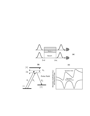
FIG. 1.: (a) Schematic of the setup to create and observe transparent anomalous dispersion; (b) atomic transition scheme for double-peaked Raman amplification; (c) refractive index and gain coefficient as a function of probe beam frequency.

Consider now the detection of a signal corresponding to a light pulse as indicated in Figure 1(a). We assign a time window $T$ centered about a pre-arranged time $t_{0}$ at the detector and monitor the photocurrent produced by the detector. We assume there is a background level of irradiation that causes a constant average photocurrent $i_{0}$ when no light pulse is received; there will be a nonvanishing $i_{0}$ whenever the medium exhibits gain. We assume further that an increased photocurrent $i_{1}(t)$ is registered when a light pulse is received, and assert that a signal has been received when the integrated photocurrent $\int dti_{1}(t)$ rises above the background level by a certain prescribed factor. The time at which this preset level of confidence is reached is then defined to be the time of arrival of this signal as recorded by an ideal detector.

The observable corresponding to this definition of the arrival time is

$$\hat{S}(L,t)=C\int_{t_{0}-T/2}^{t}dt_{1}\hat{E}^{(-)}(L,t_{1})\hat{E}^{(+)}(L,t_{1})\ ,$$ (2)

where $\hat{E}^{(+)}(L,t_{1})$ and $\hat{E}^{(-)}(L,t_{1})$ are respectively the positive- and negative-frequency parts of the electric field operator at the exit point $(z=L)$ of the medium and $T/2$ is half the time window assigned to the pulse, typically a few times the pulse width. $C$ is a constant to be specified later. The expectation value $\langle\hat{S}(L,t)\rangle$ is proportional to the number of photons that have arrived at the detector at the time $t$. If $\langle\hat{S}_{1}(L,t)\rangle$ and $\langle\hat{S}_{0}(L,t)\rangle$ are respectively the expectation values of $\hat{S}(L,t)$ with and without an input pulse, then the photocurrent difference for an ideal detector is $\langle\hat{S}_{1}(L,t)\rangle-\langle\hat{S}_{0}(L,t)\rangle$. On the other hand, the second-order variance of the integrated photon number, $\langle\Delta^{2}\hat{S}(L,t)\rangle$, gives the noise power due to quantum fluctuations. Hence it is appropriate to define an optical signal-to-noise ratio [10]

$$SNR(L,t)={(\langle\hat{S}_{1}(L,t)\rangle-\langle\hat{S}_{0}(L,t)\rangle)^{2}\over\langle\Delta^{2}\hat{S}(L,t)\rangle}\ .$$ (3)

As discussed above, we define the arrival time $t_{s}$ of a signal as the time at which $SNR(L,t)$ reaches a prescribed threshold level.

The positive-frequency part of the electric field operator can be written as

$$\hat{E}^{(+)}(z,t)=e^{-i\omega_{o}(t-z/c)}\int_{-\infty}^{\infty}dkK(\omega)\hat{a}(\omega)e^{-i\omega(t-z/v_{g})}\ ,$$ (4)

where $\omega_{o}$ is the central frequency of the pulse, $K(\omega)\propto\omega^{1/2}$, and $[\hat{a}(\omega),\hat{a}^{{\dagger}}(\omega^{\prime})]=\delta(\omega-\omega^{\prime})$. Eq. (4) assumes plane-wave propagation in the $z$ direction and that the group-velocity approximation is valid. $K(\omega)$ may for our purposes be taken to be constant since the frequency range of the two gain lines are far smaller than the central frequency $\omega_{o}$. It is then convenient to define the constant $C$ in Eq. (2) to be $1/(2\pi|K(\omega_{o})|^{2})$.

In the experiment of interest the anomalously dispersive medium is a phase-insensitive linear amplifier for which [11]

$$\hat{a}_{\rm out}(\omega)=g(\omega)\hat{a}_{\rm in}(\omega)+\sqrt{|g(\omega)|^{2}-1}\hat{b}_{\rm in}^{{\dagger}}(\omega)\ ,$$ (5)

where $\hat{a}_{\rm in}$ and $\hat{a}_{\rm out}$ refer respectively to the input ($z=0$) and output ($z=L$) ports of the amplifier and the operator $\hat{b}(\omega)$ is a bosonic operator ($[\hat{b}(\omega),\hat{b}^{{\dagger}}(\omega^{\prime})]=\delta(\omega-\omega^{\prime})$) that commutes with all operators $\hat{a}_{\rm in}(\omega)$ and $\hat{a}_{\rm in}^{{\dagger}}(\omega)$ and whose appearance in Eq. (5) is required among other things to preserve the commutation relations for the field operators $\hat{a}_{\rm out}$ and $\hat{a}^{{\dagger}}_{\rm out}$. $|g(\omega)|^{2}$ is the power gain factor characterizing the amplifier.

Now we derive a rather general expression for the optical signal-to-noise ratio. Consider first the case of propagation over the distance $L$ in a vacuum ($g(\omega)=1$). We assume that the initial state $|\psi\rangle$ of the field is a coherent state such that $\hat{a}(\omega)|\psi\rangle=\alpha(\omega)|\psi\rangle$ for all $\omega$, where $\alpha(\omega)$ is a c-number. For such a state we may write $\hat{E}^{(+)}(0,t)|\psi\rangle=\alpha(t)|\psi\rangle$, where $\alpha(t)\equiv\pi^{-1/4}(N_{p}/\tau_{p})^{1/2}\exp(-(t-T_{c})^{2}/2\tau_{p}^{2})$, $N_{p}$ is the average number of photons in the initial pulse of duration $\tau_{p}$, and $T_{c}$ is the time corresponding to the pulse peak. We obtain after a straightforward calculation the result

$$SNR(L,t)=\langle\hat{S}_{1}(0,t-L/c)\rangle_{\rm vac}=SNR(0,t-L/c)\ .$$ (6)

This expresses the expected result that the pulse propagates at the velocity $c$ with no excess noise arising from propagation.

Next we treat the case of pulse propagation over the distance $L$ in the anomalously dispersive medium, using Eq. (5) with $g(\omega)\neq 1$ and assuming again an initially coherent field. We obtain in this case

$$\langle\hat{S}_{1}(L,t)\rangle-\langle\hat{S}_{0}(L,t)\rangle=|g(0)|^{2}\langle\hat{S}_{1}(0,t-L/v_{g})\rangle_{\rm vac}$$ (7)

where $\langle\hat{S}_{0}(L,t)\rangle=(1/2\pi)\int_{T_{c}-T/2}^{t}dt_{1}\int d\omega[|g(\omega)|^{2}-1]$ is the photon number in the absence of any pulse input to the medium and $T_{c}=t_{0}-L/v_{g}$. The fact that $\langle\hat{S}_{0}(L,t)\rangle>0$ is due to amplified spontaneous emission (ASE) [10]; in the experiment of interest the ASE is a spontaneous Raman process.

Before proceeding further with the calculation of the optical signal-to-noise ratio, we note here that the gain factor

$$|g(0)|^{2}=e^{4\pi M\gamma/(\Delta\nu^{2}+\gamma^{2})\cdot L/\lambda}\ ,$$ (8)

and that the effective signal $\langle\hat{S}_{1}(L,t)\rangle-\langle\hat{S}_{0}(L,t)\rangle$ is proportional to the input signal $\langle\hat{S}_{1}(0,t-L/v_{g})\rangle_{\rm vac}$ with time delay $L/v_{g}$ determined by the group velocity $v_{g}$. In the anomalously dispersive medium $v_{g}=c/(n+\nu dn/d\nu)$ and can be $>c$ or even negative, resulting in a time delay

$${L\over v_{g}}={n_{g}L\over c}=\left[1-\nu_{o}M\cdot{\Delta\nu^{2}-\gamma^{2}\over(\Delta\nu^{2}+\gamma^{2})^{2}}\right]{L\over c}\ ,$$ (9)

which is shorter than the time delay the pulse would experience upon propagation through the same length in vacuum, or can become negative. In other words, the effective signal intensity can be reached sooner than in the case of propagation in vacuum.

In order to determine with confidence when a signal is received, however, one must evaluate the SNR. Again using the commutation relations for the field operators, we obtain for the fluctuating noise background

$$\langle\Delta^{2}\hat{S}(L,t)\rangle \equiv \langle\hat{S}^{2}(L,t)\rangle-\langle\hat{S}(L,t)\rangle^{2}$$ (10)

$$= |g(0)|^{2}\langle\hat{S}_{1}(0,t-L/v_{g})\rangle_{\rm vac}$$ (11)

$$+ 2{\rm Re}[|g(0)|^{2}\int_{t_{0}-T/2}^{t}dt_{1}\int_{t_{0}-T/2}^{t}dt_{2}$$ (12)

$$\times \alpha^{*}(t_{1}-L/v_{g})\alpha(t_{2}-L/v_{g})F(t_{1}-t_{2})]$$ (13)

$$+ \int_{t_{0}-T/2}^{t}dt_{1}\int_{t_{0}-T/2}^{t}dt_{2}|F(t_{1}-t_{2})|^{2}\ .$$ (14)

Here

$$F(t)=\int_{-\infty}^{\infty}d\omega[|g(\omega)|^{2}-1]e^{-i\omega t}$$ (15)

is a two-time correlation function for the amplified spontaneous emission noise. The three terms in Eq. (14) can be attributed to amplified shot noise, beat noise, and ASE self-beat noise, respectively [12]. The first two terms dominate in the presence of a strong input signal pulse, while the last term dominates if the input signal is small and the gain is large. In the case of a strong input signal and large gain, the second term gives the largest contribution to the noise and scales almost linearly with the signal strength $\langle\hat{S}\rangle$, the signal gain $|g(0)|^{2}$, and the peak gain $|g(\Delta\nu)|^{2}=\exp(4\pi ML/\gamma\lambda)$. This large noise term effectively reduces the signal-to-noise ratio of the advanced light pulse, causing the effective signal arrival time to be retarded by a time delay that is far larger than the pulse advancement.

Finally, using Eqs. (7) and (14), we compute $SNR^{(\rm out)}(L,t)$ for the propagation through the anomalously dispersive medium. In Figure 2 we plot the results of such computations for $SNR^{(\rm out)}(L,t)$ as a function of time on the output signal. For reference we also show $SNR$ for the identical pulse propagating over the same length in vacuum. It is evident from the results shown that the pulse propagating in vacuum maintains a higher SNR. In other words, for the experiments of interest here [7],[9], the actual arrival time of the signal is delayed, even though the pulse itself is advanced compared with propagation over the same distance in vacuum.

FIG. 2.: Signal-to-noise ratios for light pulses propagating through the gain-assisted anomalous dispersion medium $SNR(L,t)$, and through the same distance in a vacuum $SNR(0,t-L/c)$. Parameters used in the figure are adopted from the experiments reported in References [7] and [9].

By requiring that at some time $t^{\prime}$ the SNR of the output pulse be equal to that of the input pulse [Eq. (6)] at a time $t$, i.e.,

$$SNR^{({\rm out})}(L,t^{\prime})=SNR^{({\rm in})}(0,t)\ ,$$ (16)

we obtain a time difference $\delta t=t^{\prime}-t$ that marks the propagation time of the light signal, and $L/\delta t$ gives the signal velocity. In Figure 3 we plot $\delta t$ as a function of gain for $(t-T_{c})/\tau_{p}=-1,-2,$ and $-3$. This corresponds to cases where the signal point is set at 1,2, and 3 times the pulse width on the leading edge of the pulse. We also plot for reference the pulse advance $L/v_{g}$. It is evident that the retardation in the SNR far exceeds the pulse advancement. In other words, the quantum noise added in the process of advancing a signal effectively impedes the detection of the useful signal defined by the signal-to-noise ratio.

FIG. 3.: Delay $\delta t=t^{\prime}-t$ due to reduced signal-to-noise ratio as a function of the gain coefficient. Curves (a), (b), and (c) are for $t/\tau_{p}=-1,-2,$ and $-3$, respectively.

In this letter we have presented what in our opinion is a realistic definition, based on photodetections, of the velocity of the signal carried by a light pulse. We analyzed this signal velocity for the recently demonstrated superluminal light pulse propagation, and found that while the pulse and the effective signal are both advanced via propagation at a group velocity higher than $c$, or even negative, the signal velocity defined here is still bounded by $c$. The physical mechanism that limits the signal velocity is quantum fluctuation. Namely, because the transparent, anomalously dispersive medium is realized using closely-placed gain lines, the various amplified quantum fluctuations introduce additional noise that effectively reduces the SNR in the detection of the signals carried by the light pulse. This is related to the “no cloning” theorem [13],[14], which was attributed to the quantum fluctuations in an amplifier, and which is a direct consequence of the superposition principle in quantum theory.

Finally we note that it is perhaps possible to find other definitions of a “signal” velocity for a light pulse, different from that we presented here. But such a definition should in our opinion satisfy two basic criteria. First, it must be directly related to a known and practical way of detecting a signal. Second, it should refer to the fastest practical way of communicating information. While it may be hard to prove that any definition meets the second criterion, it can be hoped that the recent interest in quantum information theory might lead to a generally accepted notion of the signal velocity of light.

REFERENCES

- [1] G. Diener, Phys. Lett. A223, 327 (1996).
- [2] L. Brillouin, Wave Propagation and Group Velocity (Academic, New York, 1960).
- [3] R. Y. Chiao, in Amazing Light: A Volume Dedicated to Charles Hard Townes on His 80th Birthday, edited by R. Y. Chiao (Springer-Verlag, New York, 1996), p. 91.
- [4] In general it is not possible to define a time-of-arrival operator in quantum mechanics. See J. Oppenheim, B. Reznik, and W. G. Unruh, Phys. Rev. A59, 1804 (1999), and references therein.
- [5] Y. Aharonov, B. Reznik, and A. Stern, Phys. Rev. Lett. 81, 2190 (1998).
- [6] B. Segev, P. W. Milonni, J. F. Babb, and R. Y. Chiao, Phys. Rev. A62, 022114 (2000).
- [7] L. J. Wang, A. Kuzmich, and A. Dogariu, Nature 406, 277 (2000).
- [8] Experiments by S. Chu and S. Wong [Phys. Rev. Lett. 48, 738 (1982)] showed that can be , , or . The pulses in these experiments were strongly attenuated, and numerical simulations by B. Segard and B. Macke [Phys. Lett. 109A, 213 (1985)] indicate that they were also strongly distorted. See also A. Katz and R. R. Alfano, Phys. Rev. Lett. 49, 1292 (1982), and S. Chu and S. Wong, ibid., 1293.
- [9] A. Dogariu, A. Kuzmich, and L. J. Wang, Phys. Rev. A (to be published).
- [10] E. Desurvire, Erbium-Doped Fiber Amplifiers: Principles and Applications (Wiley, New York, 1994), Chapter 2.
- [11] H. A. Haus and J. A. Mullen, Phys. Rev. 128, 2407 (1962). See also C. M. Caves, Phys. Rev. D26, 1817 (1982).
- [12] Y. Yamamoto, IEEE J. Quantum Electron. 16, 1073 (1980).
- [13] W. K. Wooters and W. H. Zurek, Nature 299, 802 (1982).
- [14] P. W. Milonni and M. L. Hardies, Phys. Lett. A 92, 321 (1982); L. Mandel, Nature 304, 188 (1983).