Analytic solution for a class of turbulence problems

Abstract

An exact analytical method for determining the Lagrangian velocity correlation and the diffusion coefficient for particles moving in a stochastic velocity field is derived. It applies to  divergence-free 2-dimensional Gaussian stochastic fields which are stationary, homogeneous and have factorized Eulerian correlations.

Test particle motion in stochastic velocity fields is a generic problem in various topics of fluid and plasma turbulence or solid state physics [1]. The main difficulty in determining the resulting time dependent (running) diffusion coefficients and mean square displacements consists in calculating the Lagrangian velocity correlation function (LVC). This is a very complex quantity which requires the knowledge of the statistical properties of the stochastic trajectories determined by the random velocity field. The vast majority of existing works employ under various guises the Corrsin approximation [2]. The physical parameter which characterizes such process of diffusion by continuous movements is the Kubo number $K$ (defined below) which measures particle’s capacity of exploring the space structure of the stochastic velocity field before the latter changes. In the weak turbulence case $K\ll 1,$ particle motion is of Brownian type and the results are well established. In the strong turbulence case ($K>1),$ this structure of the velocity field has an important influence on the LVC and on the scaling of the diffusion coefficient in $K$. This influence is most effective in the special case of  2-dimensional divergence-free stochastic velocity fields and consists in a dynamical trapping of the trajectories in the structure of the field. The existing analytical methods completely fail in describing this process [3] and the studies usually rely on direct numerical simulations of particle trajectories [4], on asymptotic methods such as the renormalization group techniques [1] or on qualitative estimates [5]. In recent works [6] a rather different statistical approach (the decorrelation trajectory method) was proposed for determining the LVC for given Eulerian correlation of the velocity field. The case of collisional particles was treated in [7]. We prove here that, in the special case of 2-dimensional divergence-free velocity fields, under the assumptions mentioned below, this method yields the exact analytical expression of the Lagrangian velocity correlation valid for arbitrary value of the Kubo number. The assumptions concern the statistical properties of the stochastic velocity field and are rather natural for a large class of physical processes. It is considered to be a stationary and homogeneous Gaussian (normal) stochastic field, either static or time dependent with statistically independent space and time variations such that the Eulerian correlation function has a factorized structure as in Eq.(4) below.

Particle motion in a 2-dimensional stochastic velocity field is described by the nonlinear Langevin equation:

$$\frac{d{\bf x}(t)}{dt}={\bf v}({\bf x}(t),t),\qquad{\bf x}(0)={\bf 0}$$ (1)

where ${\bf x}(t)$ represents the trajectory in Cartesian coordinates ${\bf x}\equiv(x_{1},x_{2}).$ The stochastic velocity field ${\bf v}({\bf x},t)$ is  divergence-free: ${\bf\nabla\cdot v}({\bf x},t)=0$ and thus its two components $v_{1}$ an $v_{2}$ can be determined from a stochastic scalar field, the stream function (or potential) $\phi({\bf x},t)$, as:

$${\bf v}({\bf x},t)={\bf\nabla}\times\phi({\bf x},t){\bf e}_{z}=\left(\frac{\partial}{\partial x_{2}},\quad-\frac{\partial}{\partial x_{1}}\right)\phi({\bf x},t)$$ (2)

where ${\bf e}_{z}$ is the versor along the $z$ axis. The stochastic stream function $\phi({\bf x},t)$ is considered to be Gaussian, stationary and homogeneous. Since the velocity components are derivatives of $\phi({\bf x},t)$, they are Gaussian, stationary and homogeneous as well. We assume that they have zero averages:

$$\left\langle\phi({\bf x},t)\right\rangle=0,\quad\left\langle{\bf v}({\bf x},t)\right\rangle={\bf 0.}$$ (3)

The Eulerian two-point correlation function (EC) of $\phi({\bf x},t)$ is assumed to be of the form:

$$E({\bf x},t)\equiv\left\langle\phi({\bf 0},0)\,\phi({\bf x},t)\right\rangle=\beta^{2}{\cal E}({\bf x})\,h(t)$$ (4)

where $\beta$ measures  the amplitude of the stream function fluctuations and $\left\langle{}\right\rangle$ denotes the statistical average over the realizations of $\phi({\bf x},t).$ ${\cal E}({\bf x)}$ is a dimensionless function having a maximum at ${\bf x}={\bf 0}$, where its value is ${\cal E}{\bf(0})=1$, and which tends to zero as $\left|{\bf x}\right|\rightarrow\infty$. It actually depends on the dimensionless variable ${\bf x}/\lambda$, where $\lambda$ is the correlation length. $h(t)$ is a dimensionless, decreasing function of time varying from $h(0)=1$ to $h(\infty)=0$. It depends on the dimensionless ratio $t/\tau_{c}$, where $\tau_{c}$ is the correlation time. The Kubo number is defined as the ratio of the average distance covered by the particles during $\tau_{c}$ to $\lambda$ : $K=V\,\tau_{c}/\lambda$  where $V=\beta/\lambda$ measures the amplitude of the fluctuating velocity. Using the definition (2) of the velocity, the two-point Eulerian correlations of the velocity components and  the potential-velocity correlations  are obtained from $E({\bf x},t)$ as:

$$E_{11} = -\frac{\partial^{2}}{\partial x_{2}^{2}}E,\quad E_{22}=-\frac{\partial^{2}}{\partial x_{1}^{2}}E,\quad E_{12}=\frac{\partial^{2}}{\partial x_{1}\partial x_{2}}E,$$ (5)

$$E_{1\phi} = -E_{\phi 1}=-\frac{\partial}{\partial x_{2}}E,\quad E_{2\phi}=-E_{\phi 2}=\frac{\partial}{\partial x_{1}}E$$ (6)

where $E_{ij}({\bf x},t)\equiv\left\langle v_{i}({\bf 0},0)\,v_{j}({\bf x},t)\right\rangle$  and $E_{\phi i}\equiv\left\langle\phi({\bf 0},0)\,\,v_{i}({\bf x},t)\right\rangle.$

Starting from this statistical description of the stochastic stream function, we will determine the Lagrangian velocity correlation (LVC), defined by:

$$L_{ij}(t)\equiv\left\langle v_{i}({\bf x}(0),0)\,v_{j}({\bf x}(t),t)\right\rangle.$$ (7)

The mean square displacement and the running diffusion coefficient are determined by this function:

$$\left\langle x_{i}^{2}(t)\right\rangle=2\int_{0}^{t}d\tau\;L_{ii}(\tau)\;(t-\tau),$$ (8)

$$D_{i}(t)=\int_{0}^{t}d\tau\;L_{ii}(\tau).$$ (9)

For small Kubo numbers (quasilinear regime), the results are well established: the diffusion coefficient is $D_{QL}=(\lambda^{2}/\tau_{c})K^{2}.$ At large $K$ the time variation of the stochastic potential is slow and the trajectories can follow approximately the contour lines of $\phi({\bf x},t).$ This produces a trapping effect : the trajectories are confined for long periods in small regions. A typical trajectory shows an alternation of large displacements and trapping events. The latter appear when the particles are close to the maxima or minima of the stream function and consists of trajectory winding on almost closed small size paths. The large displacements are produced when the trajectories are at small absolute values of the stream function.

The main idea in our method is to study the Langevin equation (1) in subensembles (S) of the realizations of the stochastic field which are determined by given values of the stream function and of the velocity in the starting point of the trajectories:

$$\phi({\bf 0},0)=\phi^{0},\quad{\bf v}({\bf 0},0)={\bf v}^{0}.$$ (10)

The LVC for the whole set of realizations can is obtained by summing up the contributions of all subensembles (10):

$$L_{ij}(t)=\int\int d\phi^{0}\,d{\bf v}^{0}\,P_{1}(\phi^{0})\,P_{1}({\bf v}^{0})\,L_{ij}^{s}(t)$$ (11)

where $L_{ij}^{s}(t)$ is the LVC in (S) and $\,P_{1}(\phi^{0})\,$, $P_{1}({\bf v}^{0})\,$ are the Gaussian (normal) probability densities for the initial stream function and respectively for the initial velocity. As shown below, there are two important advantages determined by this procedure: (i) the LVC can be determined from one-point subensemble averages and (ii) the invariance of the stream function along the trajectory can be used for obtaining the average of the Lagrangian velocity and the LVC in (S).

The stream function and the velocity reduced in the subensemble (S) are still Gaussian stochastic fields but non-stationary and non-homogeneous and with space-time dependent average values:

$$\Phi^{S}({\bf x},t)\equiv\left\langle\phi({\bf x},t)\right\rangle_{S}=\phi^{0}\frac{E({\bf x},t)}{\beta^{2}}+v_{j}^{0}\frac{E_{j\phi}({\bf x},t)}{V^{2}},$$ (12)

$$V_{i}^{S}({\bf x},t)\equiv\left\langle v_{i}({\bf x},t)\right\rangle_{S}=\phi^{0}\frac{E_{\phi i}({\bf x},t)}{\beta^{2}}+v_{j}^{0}\frac{E_{ji}({\bf x},t)}{V^{2}}$$ (13)

where $\left\langle{}\right\rangle_{S}$ represents the average over the realizations in the subensemble (S). These averages are determined using conditional probability distribution; they are equal in ${\bf x}={\bf 0}$ and $t=0$ to the parameters determining (S): $\Phi^{S}({\bf 0},0)=\phi^{0},\;V_{i}^{S}({\bf 0},0)=v_{i}^{0}$ and decay to zero as ${\bf x}\rightarrow\infty$ and/or $t\rightarrow\infty$. A relation similar to (2) can easily be deduced:

$${\bf V}^{S}({\bf x},t)=\left(\frac{\partial}{\partial x_{2}},\quad-\frac{\partial}{\partial x_{1}}\right)\Phi^{S}({\bf x},t)$$ (14)

which shows that the average velocity in the subensemble (S) is  divergence-free: ${\bf\nabla\cdot V}^{S}({\bf x},t)=0.$ We have thus identified in the zero-average  stochastic velocity field a set of average velocities (labeled by $\phi^{0},$ ${\bf v}^{0})$ which contain the statistical characteristics of the velocity field (the correlation and the constraint imposed in the problem, i.e. the zero divergence condition). The LVC in (S) is:

$$L_{ij}^{S}(t)\equiv\left\langle v_{i}({\bf 0},0)\,v_{j}({\bf x(t)},t)\right\rangle_{S}=v_{i}^{0}\left\langle v_{j}({\bf x(t)},t)\right\rangle_{S}$$ (15)

and thus the problem reduces to the determination of the average Lagrangian velocity in each subensemble.

We consider first the static case $\phi({\bf x})$ ($\tau_{c}\rightarrow\infty,$ $K\rightarrow\infty,$ and the EC of the stream function $E({\bf x})$ is independent of time). The stream function is an invariant of the motion ($\phi({\bf x}(t))=\phi^{0}$ in each realization in (S)) and:

$$\left\langle\phi({\bf x}(t))\right\rangle_{S}=\phi^{0}$$ (16)

at any time. A deterministic trajectory ${\bf X}(t;S)$ can be defined in each subensemble (S) such that the average of the Eulerian stream function in (S) (Eq.(12)) calculated along this trajectory equals the average Lagrangian stream function (16):

$$\Phi^{S}({\bf X}(t;S))=\left\langle\phi({\bf x}(t))\right\rangle_{S}=\phi^{0}.$$ (17)

Since the Eulerian average potential (12) has the value $\phi^{0}$ in ${\bf x=0}$, the trajectory ${\bf X}(t;S)$ can be determined from the following Hamiltonian system of equations with $\Phi^{S}({\bf X})$ as Hamiltonian function:

$$\frac{d{\bf X}(t;S)}{dt}=\left(\frac{\partial}{\partial X_{2}},\quad-\frac{\partial}{\partial X_{1}}\right)\Phi^{S}({\bf X}(t;S))$$ (18)

and with the initial condition ${\bf X(}0;S)={\bf 0.}$ The trajectory in each realization in (S) can be referred to this deterministic (realization-independent) trajectory, ${\bf x}(t)={\bf X}(t;S)+\delta{\bf x}(t).$ Using the definition of the velocity (2) and expressing the space derivatives as derivatives with respect to the deterministic part of the trajectory in each realization and then averaging in the subensemble (S), the average Lagrangian velocity in (S) is obtained as:

$$\left\langle{\bf v}({\bf x}(t))\right\rangle_{S}={\bf V}^{S}\left({\bf X}(t;S)\right)$$ (19)

where Eq.(14) was used. Thus, the average Lagrangian velocity in the subensemble (S) is just the corresponding Eulerian quantity calculated along the deterministic trajectory ${\bf X}(t;S).$ Since the latter is determined by solving Eq.(18), where the r.h.s. is the average Lagrangian velocity, it follows that ${\bf X}(t;S)$ is  precisely the average trajectory in (S) :

$${\bf X}(t;S)=\left\langle{\bf x}(t)\right\rangle_{S}.$$ (20)

Similar results are obtained in the time-dependent case $\phi({\bf x},t)$ (finite $\tau_{c}$ and $K)$ if the space and time dependences are statistically independent in the sense that the EC of $\phi({\bf x},t)$ is given by Eq.(4). The stream function is not a true invariant of the motion. However the velocity is still perpendicular to ${\bf\nabla}\phi({\bf x}(t),t)$ at any moment and only the explicit time-dependence contributes to the variation of $\phi$ along the trajectory:

$$\frac{d\phi({\bf x}(t),t)}{dt}=\frac{\partial\phi({\bf x}(t),t)}{\partial t}.$$ (21)

Due to the factorized EC (4) considered here, the average Eulerian stream function and velocity (12), (13) can be written as:

$$\Phi^{S}({\bf x},t)=\Phi^{S}({\bf x})\,h(t),$$ (22)

$${\bf V}^{S}({\bf x},t)={\bf V}^{S}({\bf x})\,h(t)$$ (23)

where $\Phi^{S}({\bf x})$ and ${\bf V}^{S}({\bf x})$ are the corresponding quantities in the static case. We define in (S) a deterministic trajectory $\overline{{\bf X}}(t;S)$ as the solution of the time dependent Hamiltonian system with $\Phi^{S}(\overline{{\bf X}},t)$ as Hamiltonian function. Performing the change of variable $t\rightarrow\theta(t)=\int_{0}^{t}d\tau\,h(\tau),$ the time dependent Hamiltonian system reduces to Eq.(18) and thus the trajectory $\overline{{\bf X}}(t;S)$ can be written as:

$$\overline{{\bf X}}(t;S)={\bf X}(\theta(t);S)$$ (24)

where ${\bf X}(\theta;S)$ is the deterministic trajectory obtained in the static case. On the other hand, the average Lagrangian potential corresponding to Eq.(22) can be written as $\left\langle\phi({\bf x}(t),t)\right\rangle_{S}=G(t)\,h(t)$ where the factor $h(t)$ ”propagates” unchanged from the Eulerian average to the Lagrangian one, and $G(t)$ is the contribution of the space dependence. Taking the time derivative of this equation one obtains using Eq.(21):

$\displaystyle\frac{d}{dt}\left\langle\phi({\bf x}(t),t)\right\rangle_{S}=\mathrel{\mathop{\lim}\limits_{\delta t\rightarrow 0}}\frac{\left\langle\phi({\bf x}(t),t+\delta t)\right\rangle_{S}-\left\langle\phi({\bf x}(t),t)\right\rangle_{S}}{\delta t}.$

It follows that $d\left\langle\phi({\bf x}(t),t)\right\rangle_{S}/dt=G(t)dh/dt$ and thus $G(t)=\phi^{0}$ and the average Lagrangian stream function in (S) is:

$$\left\langle\phi({\bf x}(t),t)\right\rangle_{S}=\phi^{0}\,h(t).$$ (25)

Using Eq.(25) and (22) and the definition of    $\overline{{\bf X}}(t;S)$, one finds that the average Eulerian stream function calculated along the deterministic trajectory ${\bf\ }\overline{{\bf X}}(t;S)$ equals, as in the static case, the average Lagrangian stream function:

$$\Phi^{S}\left(\overline{{\bf X}}(t;S)\right)\,h(t)=\left\langle\phi({\bf x}(t),t)\right\rangle_{S}=\phi^{0}\,h(t)$$ (26)

Following the same arguments as in the static case, the average Lagrangian velocity in (S) is determined as:

$$\left\langle{\bf v}({\bf x}(t),t)\right\rangle_{S}={\bf V}^{S}\left(\overline{{\bf X}}(t;S)\right)\,h(t)$$ (27)

and the deterministic trajectory $\overline{{\bf X}}(t;S)$ is the average trajectory in (S):

$$\overline{{\bf X}}(t;S)=\left\langle{\bf x}(t)\right\rangle_{S}.$$ (28)

We have thus obtained the subensemble averages of the Lagrangian stream function and velocity. These averages of random functions of random arguments appear to be equal to the average functions evaluated at the average argument. We note that this surprisingly simple result which is usually wrong for stochastic functions is exact for the special case studied here. This property is essentially due to the very strong constraint imposed by the invariance of the stream function along the trajectories.

The LVC (7) and the running diffusion coefficient (9), are determined using Eqs. (11) and (15) as:

$$L_{ij}(t)=\delta_{ij}V^{2}\,F^{\prime}\left(K\theta(t)\right)\,h(t),$$ (29)

$$D(t)=\frac{\lambda^{2}}{\tau_{c}}\,K\,F\left(K\theta(t)\right)$$ (30)

where $F^{\prime}(\tau)$ is the derivative of the function $F(\tau)$ which is defined by:

$$F(\tau)\equiv\frac{1}{\sqrt{2\pi}}\int\int_{0}^{\infty}dpdu\,u^{3}\exp\left(-\frac{u^{2}(1+p^{2})}{2}\right)X(\tau;u,p).$$ (31)

$X(\tau;u,p)$ is the component of the average trajectory (normalized by $\lambda)$ along ${\bf v}^{0}$ and the dimensionless parameters $u\equiv\left|{\bf v}^{0}\right|/V,$ $p\equiv\phi^{0}/u\beta$ determine the subensemble (S). It is the solution of Eq.(18). The function $\theta$ in Eqs.(29), (30) is defined by:

$$\theta(t)=\int_{0}^{t}h(t_{1})\,dt_{1}.$$ (32)

We note that Eqs.(29)-(32) represent the exact solution for the diffusion problem studied here (both for static and time-dependent case). Two functions are involved in the expressions for the LVC and $D(t).$ One is the time dependence $h(t)$ of the EC of the stream function. This accounts for the explicit time decorrelation and remains unchanged when passing from Eulerian to Lagrangian quantities. The other is the function $F(\tau)$ which results from the space dependence of the EC of the stream function (i.e. from the Lagrangian nonlinearity). It is obtained as an integral over the subensembles (S) of the average displacements along the initial velocity ${\bf v}^{0}.$

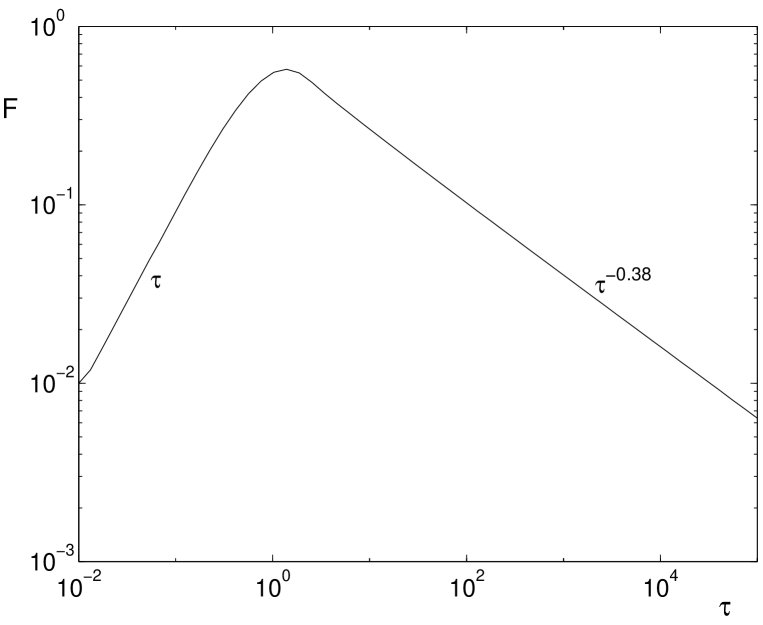
FIG. 1.: The function $F(\tau)$ defined in Eq.(31)

The trajectories obtained from Eq.(18) lie on closed paths (except for $\phi^{0}=0$ which correspond to a straight line along ${\bf v}^{0}$). The size of these paths is large for small $\left|\phi^{0}\right|$ and it decreases as $\left|\phi^{0}\right|$ increases. At small time $\tau,$ $X(\tau;u,p)\cong u\tau$ and $F(\tau)\cong\tau.$ At large time $\tau,$ the trajectory ${\bf X}(\tau;u,p)$ turns periodically along the corresponding path. The period grows with the size of the path. Thus, for a given time $\tau,$ the trajectories corresponding to small paths (large $\left|\phi^{0}\right|)$ rotate many times while those along large enough paths (small $\left|\phi^{0}\right|)$ are still opened. Consequently, when calculating the integrals in Eq.(31), the contribution of the small paths (large $\left|\phi^{0}\right|)$  is progressively eliminated as $\tau$ increases due to incoherent mixing. As $\tau$ increases, smaller and smaller intervals of $\phi^{0}$ around $\phi^{0}=0$ effectively contribute to the function $F(\tau)$ which consequently decays to zero as $\tau\rightarrow\infty.$ Thus, the function $F$ accounts for the dynamical trapping of the trajectories. The characteristic features of this self-consistent trapping process observed in the numerical simulations are recovered in the structure of this function. It shows that only a part of the trajectories (which are not yet trapped) effectively contribute to the value of the diffusion coefficient at that moment. These are the particles that move on the large size contour lines of the stochastic stream function which correspond to $\phi\cong 0.$ The trapping process is evidenced at large time and determines the decay of $F$ as $F(\tau)\sim\tau^{-\alpha}.$ The function $F(\tau)$ obtained for ${\cal E}({\bf x})=1/(1+{\bf x}^{2}/2\lambda^{2})$ is presented in Fig.1 where the two regimes are observed. The value of $\alpha$ for this case is $\alpha=0.38.$ The modification of ${\cal E}({\bf x})$ determines a variation of $\alpha$ around this value.

In a static stream function ($K,\tau_{c}\rightarrow\infty,$ $h(t)=1)$ the particles move along the ”frozen” contour lines of $\phi({\bf x})$ and the process is subdiffusive. This can easily be recovered in the general result (29)-(32). The average trajectories in the subensembles (S) are periodic functions of time and the diffusion coefficient (30) is $D(t)=\beta\,F\left(Vt/\lambda\right).$ It goes to zero when $t\rightarrow\infty$ as $D(t)=\beta\left(Vt/\lambda\right)^{-\alpha}$ and the mean square displacement is $\left\langle x^{2}(t)\right\rangle\sim t^{1-\alpha}.$

In the time dependent case, the time variation of the stream function determines a decorrelation effect which leads to a diffusive process. This is reflected in the average trajectories in the subensembles (S) (determined by Eqs.(28), (24)) which are not anymore periodic functions of time but all of them saturate as $t\rightarrow\infty$ (possibly after performing many rotations around the corresponding paths). Consequently, the decay of the function $F$ saturates at $F(K\,\theta_{\infty})$ where $\theta_{\infty}$ is a constant of order 1 obtained as the limit $t\rightarrow\infty$ of Eq.(32) and the asymptotic diffusion coefficient is:

$$D=\frac{\lambda^{2}}{\tau_{c}}K\,F\left(K\,\theta_{\infty}\right).$$ (33)

In the limit of small $K,$ the quasilinear result is recovered from Eq.(33) and at large $K$ when trapping is important $D\approx(\lambda^{2}/\tau_{c})K^{1-\alpha}.$

In conclusion, we have presented here an exact solution for the turbulent diffusion problem for a class of velocity fields. We have obtained analytical expressions for the LVC and $D(t)$ which are valid for arbitrary values of the Kubo number and describes the complicated process of dynamic trajectory trapping in the structure of the stochastic field. The basic idea of the method consists of determining the LVC by means of a set of average Lagrangian velocities estimated in subensembles of realizations of the stochastic field which are defined taking into account the invariants of the motion. It can be extended, at least as a new type of approximation, to other types of stochastic velocity fields.

This work has benefited of the NATO Linkage Grant CRG.LG 971484 which is acknowledged.

REFERENCES

- [1] J. P. Bouchaud and A. George, Phys. Reports 195, 128 (1990).
- [2] W. D. McComb, The Physics of Fluid Turbulence (Clarendon, Oxford, 1990).
- [3] R. H. Kraichnan, Phys. Fluids 19, 22 (1970).
- [4] J.-D. Reuss and J. H. Misguich, Phys. Rev. E 54, 1857 (1996); J.-D. Reuss, M. Vlad and J. H. Misguich, Phys. Lett. A 241, 94 (1998).
- [5] M. B. Isichenko, Plasma Phys. Contr. Fusion 33, 809 (1991).
- [6] M. Vlad, F. Spineanu, J. H. Misguich and R. Balescu, Phys. Rev. E 58, 7359 (1998).
- [7] M. Vlad, F. Spineanu, J. H. Misguich and R. Balescu, Phys. Rev. E 61, 3023 (2000).