2 Institute of Nuclear Research of the Hungarian Academy of Sciences, Bem tér 18/C, H–4026 Debrecen, Hungary
3 Department of Mathematical and Computational Physics, St. Petersburg State University, 198904 St. Petersburg, Petrodvoretz, Ulyanovskaya Str. 1, Russia
4 Department of Experimental Physics, University of Debrecen, Bem tér 18/A, H–4026 Debrecen, Hungary
Resonant-state solution of the Faddeev-Merkuriev integral equations for three-body systems with Coulomb-like potentials
Abstract
A novel method for calculating resonances in three-body Coulombic systems is presented. The Faddeev-Merkuriev integral equations are solved by applying the Coulomb-Sturmian separable expansion method. To show the power of the method we calculate resonances of the three- and the systems.
1 Introduction
For three-body systems the Faddeev equations are the fundamental equations. After one iteration they possess connected kernels, consequently they are effectively Fredholm integral equations of second kind. Thus the Fredholm alternative applies: at certain energy either the homogeneous or the inhomogeneous equations have solutions. Three-body bound states correspond to the solutions of the homogeneous Faddeev equations at real energies, resonances, as usual in quantum mechanics, are related to their complex-energy solutions.
The Faddeev equations were derived for short-range interactions and if we simply plug-in a Coulomb-like potential they become singular. The necessary modifications have been formulated in the Faddeev-Merkuriev theory [1] on a mathematically sound and elegant way via integral equations with connected (compact) kernels and configuration space differential equations with asymptotic boundary conditions.
Recently, one of us has developed a novel method for treating the three-body Coulomb problem via solving the set of Faddeev-Noble and Lippmann-Schwinger integral equations in Coulomb–Sturmian-space representation. The method was elaborated first for bound-state problems [2] with repulsive Coulomb plus nuclear potential, then it was extended for calculating scattering at energies below the breakup threshold [3]. Also atomic bound-state problems with attractive Coulomb interactions were considered [4]. In these calculations an excellent agreement with the results of other well established methods were found and the efficiency and the accuracy of the method were demonstrated.
More recently we have extended the method for calculating resonances in three-body systems with short-range plus repulsive Coulomb interactions by solving the Faddeev-Noble integral equations [5]. Here we solve the Faddeev-Merkuriev integral equations. This way we can handle all kind of Coulomb-like potentials, not only repulsive but also attractive ones. For illustrating the power of this method we show our previous three- results and, as novel feature, we calculate resonances in the () system.
2 Faddeev-Merkuriev integral equations
The Hamiltonian of a three-body Coulombic system reads
| (1) |
where is the three-body kinetic energy operator, stands for the possible three-body potential and denotes the Coulomb-like interaction in the subsystem . We use throughout the usual configuration-space Jacobi coordinates and . Thus only depends on (), while depends on both and coordinates ().
The physical role of a Coulomb-like potential is twofold. Its long-distance part modifies the asymptotic motion, while its short-range part strongly correlates the two-body subsystems. Merkuriev proposed to split the potentials into short-range and long-range parts in the three-body configuration space via a cut-off function ,
| (2) |
and
| (3) |
The function is defined such that it separates the asymptotic two-body sector from the rest of the three-body configuration space. On the region of the splitting function asymptotically tends to and on the complementary asymptotic region of the configuration space it tends to . Rigorously, is defined as a part of the three-body configuration space where the condition
| (4) |
is satisfied. So, in the short-range part coincides with the original Coulomb-like potential and in the complementary region vanishes, whereas the opposite holds true for . Note that for repulsive Coulomb interactions one can also adopt Noble’s approach [6], where the splitting is performed in the two-body configuration space. This approach can be considered as the limit of Merkuriev’s splitting. Then coincides with the whole Coulomb interaction and with the short-range nuclear potential.
In the Faddeev procedure we split the wave function into three components
| (5) |
where the components are defined by
| (6) |
Here is the resolvent of the long-ranged Hamiltonian
| (7) |
, and is the complex energy parameter. The wave-function components satisfy the homogeneous Faddeev-Merkuriev integral equations
| (8) |
for , where is the resolvent of the channel long-ranged Hamiltonian
| (9) |
. Merkuriev has proved that Eqs. (8) possess compact kernels for positive energies, and this property remains valid also for complex energies , .
3 Solution method
We solve these integral equations by using the Coulomb–Sturmian separable expansion approach. The Coulomb-Sturmian (CS) functions are defined by
| (10) |
with and being the radial and orbital angular momentum quantum numbers, respectively, and is the size parameter of the basis. The CS functions form a biorthonormal discrete basis in the radial two-body Hilbert space; the biorthogonal partner defined by . Since the three-body Hilbert space is a direct product of two-body Hilbert spaces an appropriate basis can be defined as the angular momentum coupled direct product of the two-body bases (the possible other quantum numbers are implicitly assumed)
| (11) |
With this basis the completeness relation takes the form
| (12) |
Note that in the three-body Hilbert space, three equivalent bases belonging to fragmentation , and are possible.
In Ref. [2] a novel approximation scheme has been proposed to the Faddeev-type integral equations
| (13) |
i.e. the short-range potential in the three-body Hilbert space is taken to have a separable form, viz.
| (14) |
where . The validity of the approximation relies on the square integrable property of the term , . Thus this approximation is justified also for complex energies as long as this property remains valid. In Eq. (14) the ket and bra states are defined for different fragmentation, depending on the environment of the potential operators in the equations. Now, with this approximation, the solution of the homogeneous Faddeev-Merkuriev equations turns into solution of matrix equations for the component vector
| (15) |
where . A unique solution exists if and only if
| (16) |
The Green’s operator is a solution of the auxiliary three-body problem with the Hamiltonian . To determine it uniquely one should start again from Faddeev-type integral equations, which does not seem to lead any further, or from the triad of Lippmann-Schwinger equations [7]. The triad of Lippmann-Schwinger equations, although they do not possess compact kernels, also define the solution in an unique way. They are, in fact, related to the adjoint representation of the Faddeev operator [8]. The Hamiltonian , however, has a peculiar property that it supports bound state only in the subsystem , and thus it has only one kind of asymptotic channel, the channel. For such a system one single Lippmann-Schwinger equation is sufficient for an unique solution [9].
The appropriate equation takes the form
| (17) |
where is the resolvent of the channel-distorted long-range Hamiltonian,
| (18) |
and . The auxiliary potential depends on the coordinate and has the asymptotic form as . In fact, is an effective Coulomb interaction between the center of mass of the subsystem (with charge ) and the third particle (with charge ). Its role is to compensate the Coulomb tail of the potentials in .
It is important to realize that in this approach to get the solution only the matrix elements are needed, i.e. only the representation of the Green’s operator on a compact subset of the Hilbert space are required. So, although Eq. (17) does not possess a compact kernel on the whole three-body Hilbert space its matrix form is effectively a compact equation on the subspace spanned by finite number of CS functions. Thus we can perform an approximation, similar to Eq. (14), on the potential in Eq. (17), with bases of the same fragmentation applied on both sides of the operator. Now the integral equation reduces to an analogous set of linear algebraic equation with the operators replaced by their matrix representations. The solution is given by
| (19) |
The most crucial point in this procedure is the calculation of the matrix elements , since the potential matrix elements and can always be calculated numerically by making use of the transformation of Jacobi coordinates. The Green’s operator is a resolvent of the sum of two commuting Hamiltonians, , where and , which act in different two-body Hilbert spaces. Thus, using the convolution theorem the three-body Green’s operator equates to a convolution integral of two-body Green’s operators, i.e.
| (20) |
where and . The contour should be taken counterclockwise around the continuous spectrum of so that is analytic in the domain encircled by .
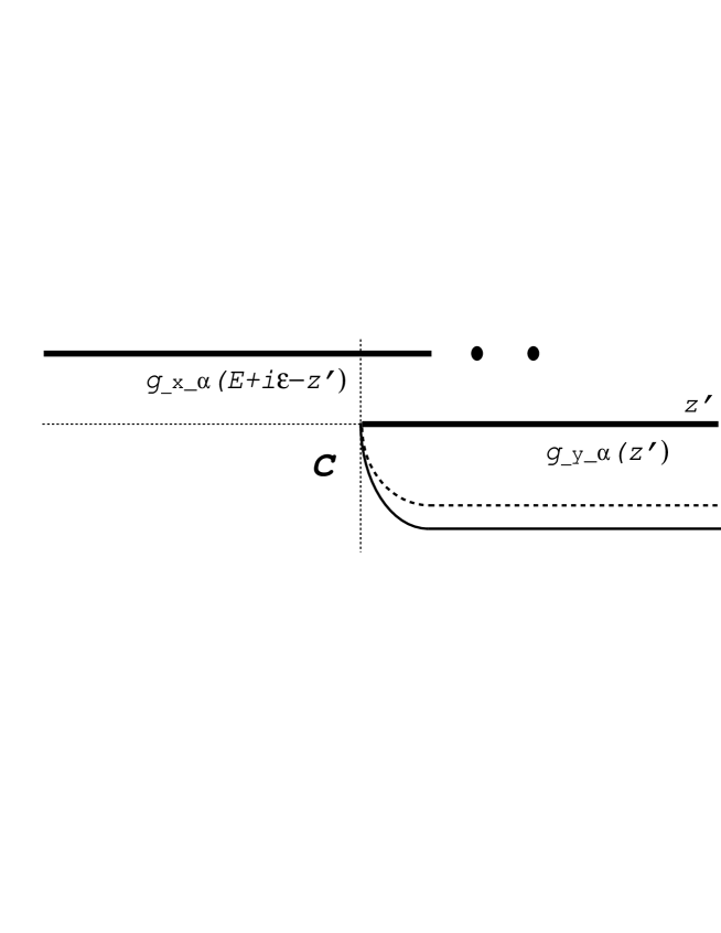
To examine the structure of the integrand let us shift the spectrum of by taking with positive . By doing so, the two spectra become well separated and the spectrum of can be encircled. Next the contour is deformed analytically in such a way that the upper part descends to the unphysical Riemann sheet of , while the lower part of can be detoured away from the cut [see Fig. 1]. The contour still encircles the branch cut singularity of , but in the limit it now avoids the singularities of . Moreover, by continuing to negative values of , in order that we can calculate resonances, the branch cut and pole singularities of move onto the second Riemann sheet of and, at the same time, the branch cut of moves onto the second Riemann sheet of . Thus, the mathematical conditions for the contour integral representation of in Eq. (20) can be fulfilled also for complex energies with negative imaginary part. In this respect there is only a gradual difference between the bound- and resonant-state calculations. Now, the matrix elements can be cast in the form
| (21) |
where the corresponding CS matrix elements of the two-body Green’s operators in the integrand are known analytically for all complex energies [10], and thus the convolution integral can be performed also in practice.
4 Numerical illustration
4.1 Resonances in a model three-alpha system
To show the power of this method we examine the convergence of the results for three-body resonant-state energies. For this purpose we take first the same model that has been presented by us before in Ref. [5]. This is an Ali–Bodmer-type model for the charged three- system interacting via -wave short-range interaction. To improve its properties we add a phenomenological three-body potential. Adopting Noble’s splitting we have
| (22) |
with MeV, MeV, fm, fm, and
| (23) |
We use units such that MeV, MeV fm. The mass of the -particle is chosen as , where denotes the mass of the nucleon. The three body potential is taken to have Gaussian form
| (24) |
where , MeV and fm. Here stands for the position vector of -th particle in the center of mass frame of the three- system. Since we consider here three identical particles we can reduce the necessary Faddeev components to one. We select states with total angular momentum . In Table 1 we show the convergence of the energy of the ground state and of the first resonant state with respect to , the number of CS functions employed in the expansion. The selected resonance is the experimentally well-known sharp state which has a great relevance in nuclear synthesis.
4.2 The system
In this system all the two-body interactions are of pure Coulomb type, two of them are attractive, therefore we have to use the genuine Merkuriev approach. Since the two electrons are identical particles we can reduce the number of Faddeev components to two. Furthermore, we can define the cutoff function such that . In this case the corresponding Faddeev component vanishes identically. So, finally we have to deal with one Faddeev component only. In the subsystem we take the Merkuriev’s cut with the functional form
| (25) |
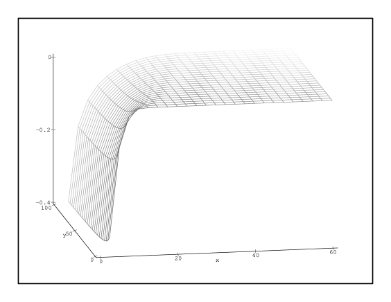
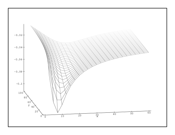
and with the actual parameters are , and . Fig. 2 and 3 show the short and long range parts of , respectively. In Table 2 we present the convergence of the energy of a resonant state with respect to and the number of angular momentum channels used in the bipolar expansion.
5 Conclusions
In this article we have presented a new method for calculating resonances in three-body Coulombic systems. The homogeneous Faddeev-Merkuriev integral equations were solved for complex energies. For this, being an integral equation approach, no boundary conditions are needed. We solve the integral equations by using the Coulomb-Sturmian separable expansion technique. The method works equally for three-body systems with repulsive and attractive Coulomb interactions.
Acknowledgments
This work has been supported by OTKA under Contracts No. T026233 and No. T029003 and by RFBR Grant No. 98-02-18190.
| 16 | -7.283744 | 0.3854244 -i 0.000011 |
|---|---|---|
| 17 | -7.283779 | 0.3851242 -i 0.000011 |
| 18 | -7.283801 | 0.3849323 -i 0.000012 |
| 19 | -7.283815 | 0.3848056 -i 0.000012 |
| 20 | -7.283824 | 0.3847236 -i 0.000012 |
| 21 | -7.283829 | 0.3846683 -i 0.000012 |
| 22 | -7.283833 | 0.3846308 -i 0.000012 |
| 23 | -7.283836 | 0.3846053 -i 0.000012 |
| 24 | -7.283837 | 0.3845873 -i 0.000013 |
| 25 | -7.283838 | 0.3845748 -i 0.000013 |
| 26 | -7.283839 | 0.3845658 -i 0.000013 |
| 27 | -7.283840 | 0.3845593 -i 0.000013 |
| 28 | -7.283840 | 0.3845546 -i 0.000013 |
| 29 | -7.283640 | 0.3845512 -i 0.000013 |
| 6 | -0.146977 -i 0.000905 | -0.146989 -i 0.000903 | -0.146991 -i 0.000902 |
|---|---|---|---|
| 7 | -0.147947 -i 0.000912 | -0.147957 -i 0.000910 | -0.147959 -i 0.000910 |
| 8 | -0.148356 -i 0.000910 | -0.148365 -i 0.000908 | -0.148367 -i 0.000908 |
| 9 | -0.148529 -i 0.000893 | -0.148538 -i 0.000892 | -0.148539 -i 0.000891 |
| 10 | -0.148608 -i 0.000882 | -0.148617 -i 0.000880 | -0.148618 -i 0.000880 |
| 11 | -0.148650 -i 0.000871 | -0.148659 -i 0.000870 | -0.148660 -i 0.000869 |
| 12 | -0.148669 -i 0.000871 | -0.148678 -i 0.000869 | -0.148680 -i 0.000869 |
| 13 | -0.148679 -i 0.000869 | -0.148688 -i 0.000868 | -0.148689 -i 0.000867 |
| 14 | -0.148683 -i 0.000870 | -0.148691 -i 0.000868 | -0.148693 -i 0.000868 |
| 15 | -0.148684 -i 0.000869 | -0.148693 -i 0.000867 | -0.148694 -i 0.000867 |
| 16 | -0.148685 -i 0.000869 | -0.148694 -i 0.000867 | -0.148695 -i 0.000867 |
| 17 | -0.148686 -i 0.000868 | -0.148695 -i 0.000867 | -0.148696 -i 0.000866 |
| 18 | -0.148686 -i 0.000869 | -0.148695 -i 0.000867 | -0.148696 -i 0.000866 |
| 19 | -0.148686 -i 0.000868 | -0.148695 -i 0.000867 | -0.148696 -i 0.000866 |
| 20 | -0.148686 -i 0.000868 | -0.148695 -i 0.000867 | -0.148696 -i 0.000866 |
References
- [1] Faddeev L. D. and Merkuriev S. P.: Quantum Scattering Theory for Several Particle Systems, (Kluver, Dordrech), (1993).
- [2] Papp Z. and Plessas W.: Phys. Rev. C 54, 50 (1996).
- [3] Papp Z.: Phys. Rev. C 55, 1080 (1997).
- [4] Papp Z.: Few-Body Systems, 24, 263 (1998).
- [5] Papp Z. Filikhin I. N. and Yakovlev S. L.: Few-Body Systems, 29, xxx (2000).
- [6] Noble J. V.: Phys. Rev. 161, 945 (1967).
- [7] Glöckle W.: Nucl. Phys. A 141, 620 (1970).
- [8] Yakovlev S. L.: Theor. Math. Phys. 102, 323 (1995); 107, 513 (1996).
- [9] Sandhas W.: Few-Body Nuclear Physics, (IAEA Vienna), 3 (1978).
- [10] Papp Z.: J. Phys. A 20, 153 (1987); Phys. Rev. C 38, 2457 (1988); Phys. Rev. A 46, 4437 (1992); Comp. Phys. Comm. 70, 426 (1992); ibid 70, 435 (1992); Kónya B., Lévai G. and Papp Z.: J. Math. Phys. 38, 4832 (1997).