SLAC-AP-134
LCC-0043
December 2000
Dipole Mode Detuning in theInjector Linacs of the NLC ***Work supported by Department of Energy contract DE–AC03–76SF00515.
Karl L.F. Bane and Zenghai Li
Stanford Linear Accelerator Center, Stanford University,
Stanford, CA 94309
Abstract
The injector linacs of the JLC/NLC project include the prelinac, the drive linac, the booster, and the booster. The first three will be S-band machines, the last one, an L-band machine. We have demonstrated that by using detuning alone in the accelerator structure design of these linacs we will have acceptable tolerances for emittance growth due to both injection jitter and structure misalignments, for both the nominal (2.8 ns) and alternate (1.4 ns) bunch spacings. For the L-band structure (a structure with phase advance) we take a uniform distribution in synchronous dipole mode frequencies, with central frequency GHz and width . For the S-band case our optimized structure ( a structure) has a trapezoidal dipole frequency distribution with GHz, , and tilt parameter . The central frequency and phase advance were chosen to put bunches early in the train on the zero crossing of the wake and, at the same time, keep the gradient optimized. We have shown that for random manufacturing errors with rms 5 m, (equivalent to error in synchronous frequency), the injection jitter tolerances are still acceptable. We have also shown that the structure alignment tolerances are loose, and that the cell-to-cell misalignment tolerance is m. Note that in this report we have considered only the effects of modes in the first dipole passband.
Dipole Mode Detuning in theInjector Linacs of the NLC
1 Introduction
A major consideration in the design of the accelerator structures in the injector linacs of the JLC/NLC[1][2] is to keep the wakefield effects within tolerances for both the nominal (2.8 ns) and the alternate (1.4 ns) bunch spacings. One important wakefield effect in the injector linacs is likely to be multi-bunch beam break-up (BBU). With this effect a jitter in the injection conditions of a bunch train, due to the dipole modes of the accelerator structures, is amplified in the linac. By the end of the linac bunches in the train are driven to large amplitudes and/or the projected emittance of the train becomes large, both effects which can hurt machine performance. Another important multi-bunch wakefield effect that needs to be considered is static emittance growth caused by structure misalignments.
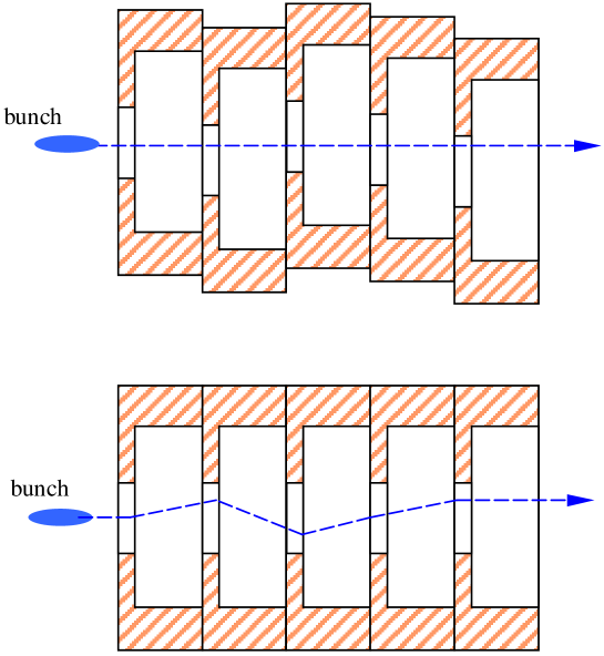
To minimize the multi-bunch wakefield effects in the injector linacs we need to minimize the sum wake in the accelerator structures. The dipole wake amplitude of the structures—and therefore also the sum wake amplitude—scales as frequency to the -3 power. Therefore, compared to the main (X–band) linac, the injector linac wakes tend to be smaller by a factor and , respectively, for the S– and L–band linacs. We shall see, however, that—in the S-band case—this reduction, by itself, is not sufficient. Two ways of reducing the sum wake further are to detune the first pass-band dipole modes and to damp them. Detuning can be achieved by gradually varying the dimensions of the cells in a structure. Weak damping can be achieved by letting the fields couple to manifolds running parallel to the structure (as is done in the main JLC/NLC linac[3]); stronger damping by, for example, introducing lossy material in the cells of the structure.
In the injector linacs the dipole mode frequencies are much lower than in the main linac, and the number of dipole mode oscillations between bunches is much smaller (see Table 1). Therefore, significantly reducing the wake envelope at one bunch spacing behind the driving bunch by detuning alone becomes more difficult. In addition, for a given , the effective damping is 4 (or 8) times less effective than for X-band.
| Scaling | ns | ns | ||||
|---|---|---|---|---|---|---|
| Band | Freq. | Wake | ||||
| X | 1 | 1 | 42.0 | 132 | 21.0 | 66 |
| C | 1/2 | 1/8 | 21.0 | 66 | 10.5 | 33 |
| S | 1/4 | 1/64 | 10.5 | 33 | 5.3 | 16 |
| L | 1/8 | 1/512 | 5.3 | 16 | 2.6 | 8 |
In this report our goal is to design the accelerator structures for the injector linacs using simple detuning alone, i.e. including no damping, to take care of the long-range wakefields. We focus mostly on the S-band injector linacs. We begin by discussing analytical approaches to estimating the effects of BBU and structure misalignments. We then discuss wakefield compensation using detuning. We optimize structure dimensions for structures with and per cell phase advance, and show that the latter is preferable. And finally we obtain tolerances to wakefield effects for all the injector linacs using both analytical formulas and numerical tracking. Note that in this report we are only concerned with the effects of modes in the first dipole passband, which have kick factors much larger than those in the higher passbands. The effects of the higher passband modes, however, will need to be addressed in the future.
2 Emittance Growth
2.1 Beam Break-up (BBU)
In the case of single-bunch beam break-up in a linac the amplification of injection jitter can be characterized by a strength parameter dependent on the longitudinal position within the bunch. When the strength parameter is sufficiently small the growth in amplitude at the end of the linac is given by the first power of this parameter[4]. For the multi-bunch case we can derive an analogous strength parameter, one dependent on bunch number . When this strength parameter is sufficiently small we expect that again the growth in amplitude at the end of the linac is given by the first power of the parameter. (But even when the strength parameter is not sufficiently small it can be a useful parameter for characterizing the strength of BBU.) For the multi-bunch case the strength parameter becomes (see Appendix A)
| (1) |
with the single bunch population, the machine length, the initial value of the beta function averaged over a lattice cell, the initial energy, the final energy, and the number of bunches in a train. The sum wake is given by
| (2) |
with the transverse wakefield and the time interval between bunches in a train. The wakefield, in turn, is given by a sum over the dipole modes in the accelerator structures:
| (3) |
with the number of modes, , , and are, respectively, the frequency, the kick factor, and the quality factor of the mode. The function in Eq. 1 is one depending on the energy gradient and focusing profile in the linac. For acceleration assuming the beta function varies as ,
| (4) |
If , for all , is not large, the linear approximation applies, and this parameter directly gives the (normalized) growth in amplitude of bunch . If is not large the projected normalized emittance growth of the bunch train becomes (assuming, for simplicity, that, in phase space, the beam ellipse is initially upright):
| (5) |
with the initial bunch offset, the rms of the strength parameter (the square root of the second moment: the average is not subtracted), and the initial beam size. Note that the quantity in the multi-bunch case takes the place of the bunch wake (the convolution of the wake with the bunch distribution) in the single bunch instability problem. As jitter tolerance parameter, , we can take that ratio that yields a tolerable emittance growth, .
2.2 Misalignments
If the structures in the linac are (statically) misaligned with respect to a straight line, the beam at the end of the linac will have an increased projected emittance. If we have an ensemble of misaligned linacs then, to first order, the distribution in emittance growth at the end of these linacs is given by an exponential distribution , with[5] 222This equation is a slightly generalized form of an equation given in Ref. [5].
| (6) |
with the structure length, the rms of the structure misalignments, is the rms of the sum wake with respect to the average, the number of structures; the function is given by (again assuming ):
| (7) |
Eq. 6 is valid assuming the so-called betratron term in the equation of motion is small compared to the misalignment term.
We can define a misalignment tolerance by
| (8) |
with the tolerance in emittance growth. What is the meaning of ? For an ensemble of machines, each with a different collection of random misalignment errors but with the same rms , then the distribution of final emittances will be given by the exponential function with expectation value . Note that if we, for example, want to have 95% confidence to achieve this emittance growth, we need to align the machine to a tolerance level of .
Besides the tolerance to structure misalignments, we are also interested in the tolerance to cell-to-cell misalignments due to fabrication errors. A structure is built as a collection of cups, one for each cell, that are brazed together, and there will be some error, small compared to the cell dimensions, in the straightness of each structure. To generate a wake (for a beam on-axis) in a structure with cell-to-cell misalignments we use a perturbation approach that assumes that, to first order, the mode frequencies remain unchanged (from those in the straight structure), and only new kick factors are needed[6] (The method is described in more detail in Appendix B). Note that for particle tracking through structures with internal misalignments, contributions from both this (orbit independent) wake force and the normal (orbit dependent) wake force need to be included.
Machine properties for the injector linacs used in this report are given in Table 2[2]. The rf frequencies of all linacs are sub–harmonics of the main linac frequency, 11.424 GHz. The prelinac, drive linac, booster linac all operate at S–band (2.856 GHz), and the booster linac at L–band (1.428 GHz). Note that and are only a rough fitting of the real machine –function to the dependence . In Table 3 beam properties for the injector linacs, for the nominal bunch train configuration (95 bunches spaced at ns), are given. For the alternate configuration (190 bunches spaced at ns) is reduced by .
| Name | Band | [GeV] | [GeV] | [m] | [m] | |
|---|---|---|---|---|---|---|
| Prelinac | S | 1.98 | 10.0 | 558 | 8.6 | 1/2 |
| Drive | S | .08 | 6.00 | 508 | 2.4 | 1/2 |
| Booster | S | .08 | 2.00 | 163 | 3.4 | 1/4 |
| Booster | L | .25 | 2.00 | 184 | 1.5 | 1 |
| Name | [mm] | [%] | [m] | |
|---|---|---|---|---|
| Prelinac | 1.20 | 0.5 | 1. | |
| Drive | 1.45 | 2.5 | 1. | |
| Booster | 1.45 | 2.5 | 1. | |
| Booster | 1.60 | 9.0 | 3.5 |
3 Wakefield Compensation
For effective detuning, one generally requires that the wake amplitude drop quickly, in the time interval between the first two bunches, and then remain low until the tail of the bunch train has passed. In the main (X-band) linac of the NLC, Gaussian detuning is used to generate a fast Gaussian fall-off in the wakefield; in particular, at the position of the second bunch the wake is reduced by roughly 2 orders of magnitude from its initial value. The short time behavior of the wake can be analyzed by the so-called “uncoupled” model. According to this model (see, for example, Ref. [8])
| (9) |
where is the number of cells in the structure, and and are, respectively, the frequency and kick factor at the synchronous point, for a periodic structure with dimensions of cell . Therefore, one can predict the short time behavior of the wake without solving for the modes of the system. (In the following we will omit the unwieldly subscript ; whether the synchronous or mode parameters are meant will be evident from context.)
For Gaussian detuning the initial fall-off of the wake is given by
| (10) |
with the average kick factor, the average (first band) synchronous, dipole mode frequency, and the sigma parameter in the Gaussian distribution. Suppose we want a relative amplitude reduction to 0.05 at the position of the second bunch. Considering the alternate (1.4 ns) bunch spacing, and taking GHz (S-band), we find that the required . To achieve a smooth Gaussian drop–off of the wake requires that we take at least as the full–width of our frequency distribution, a number which is clearly too large.
If we limit the total frequency spread to an acceptable and keep the parameter fixed, our Gaussian distribution becomes similar to a uniform distribution. For the case of a uniform distribution with full width the wake becomes
| (11) |
Again considering S-band with the alternate (1.4 ns) bunch spacing, and taking GHz, we obtain an amplitude reduction to 0.37 at the position of the second bunch, which is still too large. If we want to substantially reduce the wake further we need to shift the average dipole frequency , so that the term in Eq. 11 becomes small, and the wake at the second bunch is near a zero crossing. That is,
| (12) |
with the bunch spacing. With an even integer the bunch train will be near the integer resonance, otherwise it will be near the half-integer resonance. With our parameters , and Condition 12 is achieved by changing by (or by a much larger amount in the positive direction). However, GHz is the average dipole mode frequency for the somewhat optimized structure, and a change of results in a net loss of 7% in accelerating gradient, and, presumably, a 7% increase in the required lengths of the S–band injector linacs. One final possibility for reducing the wake at one bunch spacing is to introduce heavy damping. But for this case, just to reduce the wake at one bunch spacing by , a quality factor of 16 would be needed (see Table 1), and such a quality factor is not easy to achieve without a significant loss in fundamental mode shunt impedance.
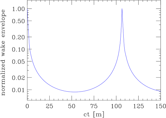
The wakefield for a uniform distribution, as given by Eq. 11, not only gives the initial drop-off of the wake, but also the longer term behavior. (However, here the mode parameters, not the synchronous parameters, are needed. Therefore, to see whether such a mode distribution can actually be achieved the circuit equations need to be solved.) We see that for a uniform distribution the wakefield resurges to a maximum again, at . Therefore, must be sufficiently small to avoid this resurgence occurring before the end of the bunch train; i.e. it must be significantly less than (which is about 10% in our case). The envelope of Eq. 11 for , GHz, and is shown in Fig. 1.
Another possibility for pushing the resurgence in the wake to larger is to use two structure types, which can effectively double the number of modes available for detuning. This idea has been studied; it has been rejected in that it requires extremely tight alignment tolerances between pairs of such structures.
3.1 Phase Advance Per Cell
Except for the region of the initial drop-off, we need to solve for the eigenmodes of the system to know the behavior of the wake or the sum wake for a detuned structure. To numerically obtain these modes we use a computer program that solves the double-band circuit model described in Ref. [8]. We consider structures of the disk–loaded type, with constant period and with rounded irises of fixed thickness. The iris radii and cavity radii are adjusted to give the correct fundamental mode frequency and the desired dipole mode spectrum. Therefore, the dimensions of a particular cell can be specified by one free parameter, which we take to be the synchronous frequency of the first dipole mode pass band, (more precisely, the synchronous frequency of the periodic structure with cell dimensions of cell ). The computer program generates coupled mode frequencies and kick factors , with the number of cells in a structure. It assumes the modes are trapped at the ends of the structure. Only the modes of the first band (approximately the first modes) are found accurately by the two-band model. And since, in addition, the strengths of the first band modes are much larger than those of the second band (in the S-band case the synchronous mode kick factors are larger by a factor ), we will use only the first band modes to obtain the wake, and then the sum wake.
For our S-band structures, we will consider a uniform frequency distribution, with a central frequency chosen so that at one bunch spacing, for the alternate configuration ( ns), the wake is very close to a zero crossing. The strength of interaction with the modes, given by the kick factors , will be stronger near the downstream end of the structure, where the iris radii become smaller. To counteract this asymmetry we will allow the top of the frequency distribution to be slanted at an angle, and therefore, our distribution becomes trapezoidal in shape. We parameterize this slant by
| (13) |
where is the synchronous frequency distribution, and and represent, respectively, the lowest and highest frequencies in the distribution. Note that . With , , and the relative width of the distribution , we have 3 parameters that we will vary to reduce the wakefield effects—specifically by minimizing on the sum wake—for both bunch train configurations.
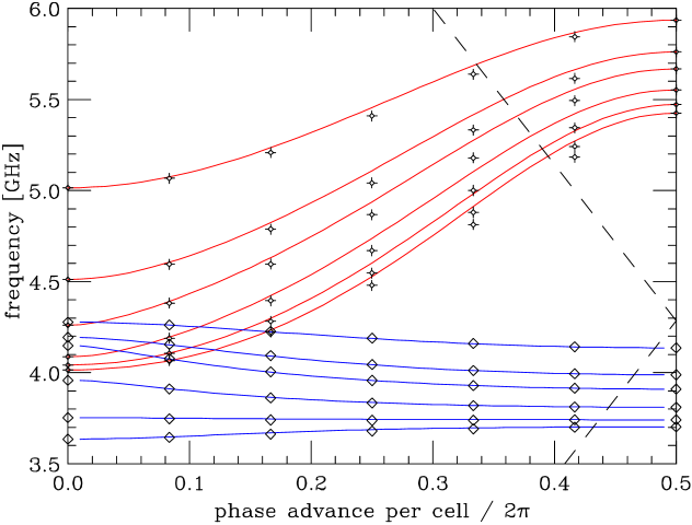
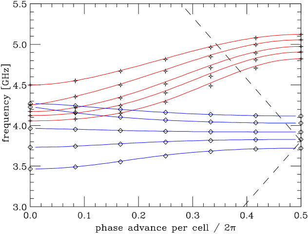
Each S-band structure operates at a fundamental mode frequency of 2.856 GHz, and consists of 114 cells with a cell period of 3.5 cm (where the phase advance per cell ), an iris thickness of 0.584 cm, and cavity radius cm. The of the modes due to wall losses (copper) . Given our implementation of the SLED-I pulse compression system[9], to optimize the rf efficiency the average (synchronous) dipole mode frequency needs to be 4.012 GHz. Fig. 2 shows the dispersion curves of the first two dipole bands for representative constant impedance, S-band structures, with varying from 1.30 cm to 2.00 cm. The results of a finite element, Maxwell Equations solving program, OMEGA2[10], are given by the plotting symbols. The end points of the curves are used to fix the parameters in the circuit program. The two-band circuit results for these constant impedance structures are indicated by the curves in the figure. We note good agreement in the first band results and not so good agreement in those of the second band. For a detuned structure, to obtain the local circuit parameters, we interpolate from these representative dispersion curves.
We have 3 parameters to vary in our input (uncoupled) frequency distribution: the (relative) shift in average frequency from the nominal 4.012 GHz, , the (relative) width of the distribution , and the flat-top tilt parameter . Varying these parameters we calculate , , and the peak value of , , for the coupled results, for both bunch train configurations. These parameters serve as indicators, respectively, of emittance growth due to BBU (injection jitter), emittance growth due to misalignments, and the maximum beam excursion due to BBU. From our numerical simulations we find that a fairly optimized case consists of , , and .
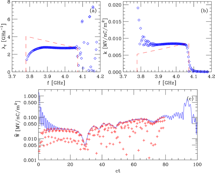
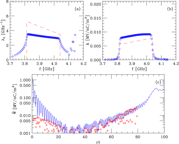
In Fig. 3 we display, for the optimized case, the frequency distribution (a), the kick factors (b), and the envelope of the wake (c). The dashed curves in (a) and (b) give the uncoupled (input) values. The plotting symbols in (c) give at the bunch positions for the alternate (1.4 ns) bunch train configuration. From (b) we note that there are a few modes, trapped near the beginning of the structure, which have kick factors significantly larger than the rest. This is a consequence of the fact that, for all cells of this structure, the dispersion curves are backward waves. From (c) we see that, due to these few strong modes, the wake envelope does not nearly reach the low, flat bottom that it does for the idealized, uniform frequency distribution (see Fig. 1). We note, however, that the short-range drop-off is similar to the idealized form (see Fig. 1), for about 20 m. In addition we note that, by setting the second bunch near the zero crossing, many following bunches also have wakes with amplitudes significantly below the wake envelope. Finally, in Fig. 4 we present the sum wake for both bunch train configurations. For this case, for both bunch train configurations, MV/nC/m2. Note that if we set back to 0, then, for the 1.4 ns bunch spacing option, becomes a factor of 20 larger.
3.2 Phase Advance Per Cell
If we would like to regain some of the 7% in accelerating gradient that we lost by shifting , we can move to a structure where the group velocity at the synchronous point is less than for the structure (for the same ). One solution is to go to a structure with a synchronous point. Note that in such a structure the cell length is 3.94 cm and that there are 102 cells per structure. Note also that for the same group velocity for the fundamental mode a higher phase advance implies larger values of iris radius , which will also improve the short-range wakefield tolerances. The dispersion curves are shown in Fig. 5. Note that, in this case, our distribution will have for the cell geometries near the beginning of the structure, for the cell geometries near the end of the structure, while the synchronous phase is near pi phase advance. Consequently modes touching either end of the structure will only weakly interact with the beam (see, eg Ref. [8]), allowing us to have a smoother impedance function, and therefore a more uniformly suppressed wakefield envelope. This was not the case for structure, where the dispersion curves for all cells have a negative slope (between 0 and phase advance) (see Fig. 2); it is also not the case for a structure, where the slopes would all be positive.
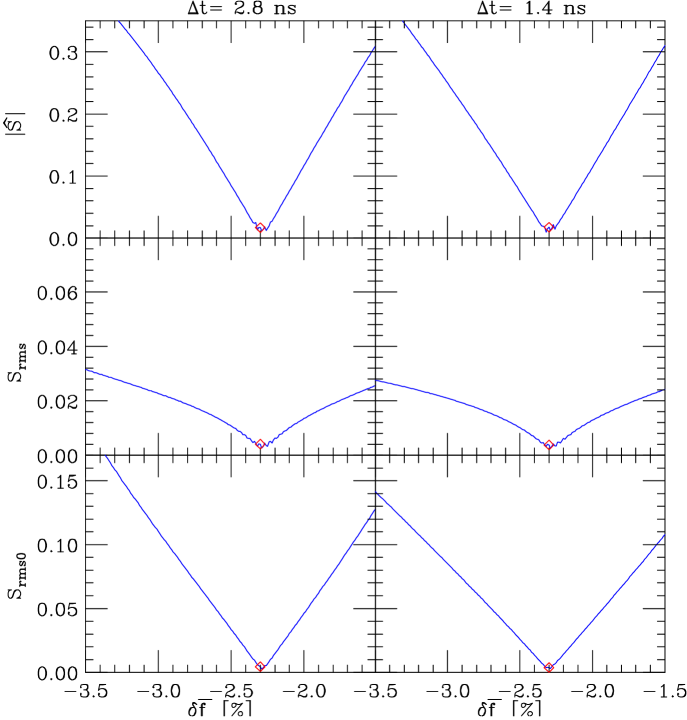
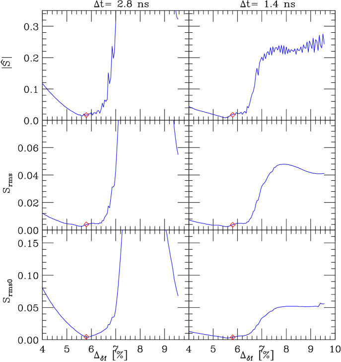
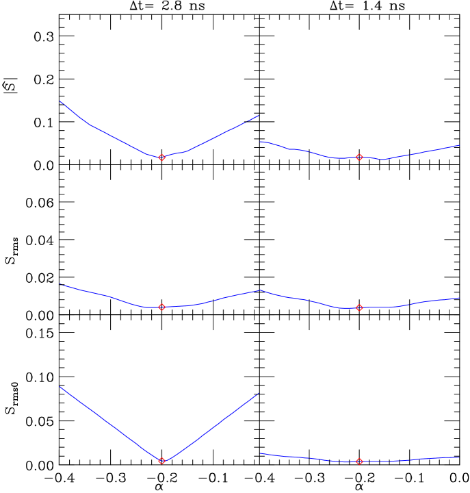
Again optimizing on the sum wake, we find that for a fairly optimized case , , and . The change of the indicators , and as we deviate from this point, for both bunch train configurations, is shown in Figs. 6-8. In Fig. 6 we show the dependence. We see that, for both bunch train configurations the results are very sensitive to . In Fig. 7 we give the dependence. We can clearly see the effect of the resurgence in the wake when . And finally, in Fig. 10 we give the dependence. We note that the tilt in the distribution helps primarily in reducing the sensitivity to BBU for the nominal (2.8 ns) bunch train configuration.
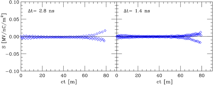
In Fig. 9 we display, for the optimized case, the frequency distribution (a), the kick factors (b), and the envelope of the wake (c). From (b) we note that in this case is a relatively smooth function, as was expected from our earlier discussion. From (c) we see that the wake envelope reaches a broader, flatter bottom than for the structure, again as we expected. Again we note that many of the earlier bunches have wakes with amplitudes significantly below the wake envelope. Finally, in Fig. 9 we show the sum wake for both bunch train configurations. The rms of these sum wakes are much smaller than for the structure: MV/nC/m2.
3.3 Frequency Errors
How sensitive are our results to manufacturing errors? We will begin to explore this question by looking at the dependence of the sum wake on errors in the synchronous frequencies of the cells of the structure. Note that the synchronous frequency of a cell is not equally sensitive to each of the cell dimensions. Basically there are 4 dimensions: the iris radius , the cavity radius , the iris thickness , and the period length . The synchronous frequency is insensitive to and , and for the average S-band cell we find that and . Or, a micron change in results in ; a micron change in results in . As for attainable accuracy, let us assume that each synchronous frequency can be obtained to a relative accuracy of , or to about .5 MHz.
As for systematic frequency errors we note from Fig. 6 that we are especially sensitive to changes in average frequency. For example, to double from its minimum, requires a relative frequency change of only . If each cell frequency has an accuracy of , and there are about 100 cells, the accuracy in the centroid frequency should be . Therefore, the effect of this type of systematic error should be negligible.
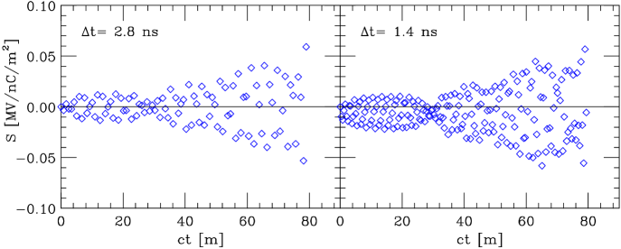
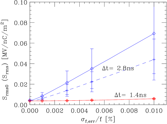
As for random manufacturing errors, let us distinguish two types: “systematic random” and “purely random” errors. By “systematic random” we mean errors, random in one structure, that are repeated in all structures of the prelinac subsystem. “Purely random” errors are, in addition, random from structure to structure. In Fig. 11 we give the resulting and , for both bunch train configurations, when a random error component is added to the (input) synchronous frequencies of the optimal distribution. With a frequency spacing of , an rms frequency error of is a relatively small perturbation. We see that for the alternate (1.4 ns) bunch spacing the effect of such a perturbation is indeed very small, whereas for the nominal (2.8 ns) bunch spacing the effect is large. The reason is that with the 1.4 ns bunch spacing the beam sits near a half-integer resonance, whereas for the 2.8 ns spacing it sits near the integer resonance. (Resonant multi-bunch wakefield effects are discussed in Appendix C.) Note, however, that if we consider the case of “purely random” machining errors, with a relative accuracy in synchronous frequencies of , and considering we have , 127, 41 structures in, respectively, the prelinac, the drive linac, and the booster, then, with a reduction in sensitivity, the appropriate abscissas in the figure become .8, .9, and . At these points, for the 2.8 ns spacing, we see that is only a factor , , times larger than the zero error result. Finally, as for the “systematic random” errors, it is difficult to judge how large they might be in the real structure; however, they are likely an order of magnitude less than the purely random errors, and should therefore not yield a sum wake much larger than that due to the purely random manufacturing errors.
If we make a weak damping, approximate calculation, by redoing the calculation but now with , we find no appreciable effect on the resonance behavior for the ns case with frequency errors. For strong damping, taking , however, we do find a suppression of the resonance effect.
3.4 Booster
For the booster (the L–band machine) each accelerator structure consists of 72 cells and the synchronous phase advance is taken to be . The synchronous dipole mode distribution is taken to be uniform, with GHz and . We take . Note that in this case ; for the second bunch to sit on the zero crossing of the wakefield would require a shift in frequency of or . For the L-band structure not much can be gained by changing the frequency spectrum. We do gain, however, a factor of 8 reduction in wake in going from S- to L-band, which, as we shall see, suffices.
4 Tolerances
For our designed structures we perform the tolerance calculations presented in Section 2. To check the analytical estimates, tracking, using the computer program LIAR[11], was also performed. The numerical simulations were simplified in that one macro-particle was used to represent each bunch, and the bunch train was taken to be mono–energetic. The analytical BBU results and those of LIAR, at the end of the four injector linacs, are compared in Table 4. Results are given for bunch spacings of 1.4 and 2.8 ns. Under the heading “Analytical” are given the rms of the sum wake , the rms of the growth factor , the maximum (within the bunch train) of the growth factor , and the tolerance for , i.e. that ratio that results in 10% emittance growth. Under the heading “Numerical” we give the LIAR results: the maximum (within the bunch train) growth in normalized phase space and the tolerance for 10% emittance growth, both referenced to the centroid of the first bunch in the train.
| Analytical | Numerical | ||||||
| Name | |||||||
| Prelinac | .004 | .007 | .025 | 70 | .020 | 85 | |
| Drive | .004 | .017 | .066 | 25 | .047 | 35 | |
| 2.8ns | Booster | .004 | .009 | .036 | 50 | .026 | 65 |
| Booster | .12 | .119 | .227 | 3.8 | .153 | 5.5 | |
| Prelinac | .004 | .004 | .019 | 115 | .015 | 140 | |
| Drive | .004 | .011 | .049 | 45 | .035 | 60 | |
| 1.4ns | Booster | .004 | .006 | .027 | 80 | .019 | 105 |
| Booster | .30 | .205 | .379 | 2.2 | .257 | 3.0 | |
| Analytical | Numerical | |||
| Name | [mm] | |||
| Prelinac | .004 | 2.9 | 3.2 | |
| Drive | .004 | 100. | 120. | |
| 2.8ns | Booster | .004 | 140. | 170. |
| Booster | .022 | 590. | ||
| Prelinac | .004 | 4.6 | 4.8 | |
| Drive | .004 | 150. | 180. | |
| 1.4ns | Booster | .004 | 210. | 260. |
| Booster | .040 | 450. | ||
We note from Table 4 that for the S-band machines, and are both small compared to 1, and that the injection jitter tolerance for 10% emittance growth is very large. For the L-band machine, the booster, the tolerances are tighter but still acceptable. We note also that the analytical agrees well with the numerical , as do the two versions of .
In Table 5 we present misalignment results. Given are and the tolerance for structure misalignments, , both as given analytically and by LIAR. As discussed before, the meaning of is the rms misalignment that (for an ensemble of machines) results, on average, in a final emittance growth equal to a tolerance , which in this case we set to 10%. From Table 5 we see that the analytical and numerical results agree well, and that the misalignment tolerances are all very loose. The tightest tolerance is for the prelinac with nominal (2.8 ns) bunch spacing, where the tolerance is still an acceptable 3 mm.
The effect of machining errors will tighten these tolerances for the S-band machines with the nominal (2.8 ns) bunch spacing, due to the beam being near the integer resonance. If machining adds a purely random error component that is equivalent to frequency error, we saw earlier that (for the 2.8 ns bunch spacing case only) this will tighten the injection jitter tolerances by about a factor for the prelinac and drive linac, and about a factor of for the booster. But even with this, the tolerances are still very loose. The misalignment tolerances are affected less by machining errors. The prelinac tolerance, with 2.8 ns bunch spacing, will become mm; for 95% confidence in achieving , the tolerance becomes mm.
Finally, what is the random, cell-to-cell misalignment tolerance? Performing the perturbation calculation described in Appendix B, and calculating for 1000 different random structures, we find that MV/nC/m2 for ns, and MV/nC/m2 for ns. We again see the effect of the integer resonance on the 2.8 ns option result. (To verify that this is the case, we performed one run but with the bunch spacing changed so that the beam sits near the next half-integer resonance (11.5); the result was that dropped by a factor of 6.) For the prelinac the cell-to-cell misalignment tolerance becomes 40 m for the nominal (2.8 ns) bunch configuration and 600 m for the alternate (1.4 ns) configuration.
5 Conclusion
We have demonstrated that by using detuning alone, the four injector linacs can be built to sufficiently suppress the multi-bunch wakefield effects, for both the nominal (2.8 ns) and alternate (1.4 ns) bunch spacings. We have studied the sensitivity to multi-bunch beam break-up (BBU) and to structure misalignments through analytical estimates and numerical tracking, and shown that the tolerances to injection jitter, in the former case, and to structure misalignments, in the latter case, are not difficult to achieve. We have also studied the effect of manufacturing errors on these tolerances, and have shown that if the errors are purely random, with an equivalent rms frequency error of , then the other tolerances are still acceptable. Finally, we have shown that the cell-to-cell misalignment tolerance is m.
For the L–band machine—the Booster—we have shown that a uniform detuning of the dipole modes, with central frequency GHz and a total frequency spread , suffices. For the S–band linacs—the Prelinac, the Drive Linac, and the Booster—we have shown that the 1.4 ns bunch spacing option forces us to reduce the central frequency by 2.3% from the nominal 4.012 GHz. Doing this we lose 7% in effective gradient, which, however, can be regained by increasing the phase advance per cell from to . Our final, optimized distribution is trapezoidal in shape with GHz, %, and tilt parameter .
We have demonstrated in this report that the integer resonance, which we cannot avoid given the two bunch train alternatives, can make us more sensitive to manufacturing errors. Also, we have shown that the analytical, single-bunch beam break-up theory, when slightly modified, can be useful in predicting the behavior of multi-bunch beam break-up also. Given the rather loose tolerances demonstrated here makes us think that the S-band machines can be replaced with C-band ones that still have reasonable tolerances, an option which may result in savings in cost, though this needs further study. Finally, we should reiterate that in this report we were concerned with the effects of the modes in the first dipole passband only. With the wakefield of the first band modes greatly suppressed by detuning, the effects of the higher bands may no longer be insignificant. This problem will need to be addressed in the future.
Acknowledgments
The author thanks the regular attendees of the Tuesday JLC/NLC linac meetings at SLAC for helpful comments and discussions on this topic, and in particular T. Raubenheimer, our leader, and V. Dolgashev for carefully reading parts of this manuscript.
References
- [1] NLC ZDR Design Report, SLAC Report 474, 589 (1996).
- [2] See the JLC/NLC Accelerator Physics at SLAC web site at: www-project.slac.stanford.edu/lc/local/AccelPhysics/Accel_Physics_index.htm.
- [3] R. M. Jones, et al, “Equivalent Circuit Analysis of the SLAC Damped Detuned Structures,” Proc. of EPAC96, Sitges, Spain, 1996, p. 1292.
- [4] A. Chao, “Physics of Collective Instabilities in High-Energy Accelerators”, John Wiley & Sons, New York (1993).
- [5] K. Bane, et al, “Issues in Multi-Bunch Emittance Preservation in the NLC,” Proc. of EPAC94, London, England, 1994, p. 1114.
- [6] R. M. Jones, et al, “Emittance Dilution and Beam Breakup in the JLC/NLC,” Proc. of PAC99, New York, NY, 1999, p. 3474.
- [7] V. Dolgashev, et al, “Scattering Analysis of the NLC Accelerating Structure,” Proc. of PAC99, New York, NY., 1999, p. 2822.
- [8] K. Bane and R. Gluckstern, Part. Accel., 42, 123 (1994).
- [9] Z. Li, et al, “Parameter Optimization for the Low Frequency Linacs in the NLC,” Proc. of PAC99, New York, NY, 1999, p. 3486.
- [10] X. Zhan, “Parallel Electromagnetic Field Solvers ,” PhD Thesis, Stanford University, 1997.
- [11] R. Assmann, et al, LIAR Reference Manual, SLAC/AP-103, April 1997.
- [12] R. Helm and G. Loew, Linear Accelerators, North Holland, Amsterdam, 1970, Chapter B.1.4.
- [13] E. U. Condon, J. Appl. Phys. 12, 129 (1941).
- [14] P. Morton and K. Neil, UCRL-18103, LBL, 1968, p. 365.
- [15] K.L.F. Bane, et al, in “Physics of High Energy Accelerators,” AIP Conf. Proc. 127, 876 (1985).
- [16] K. Bane and B. Zotter, Proc. of the 11th Int. Conf. on High Energy Acellerators, CERN (Birkhäuser Verlag, Basel, 1980), p. 581.
- [17] D. Schulte, presentation given in an NLC Linac meeting, summer 1999.
Appendix A: Analytical Formula for Weak Multi-Bunch BBU
In Ref. [4] an analytical formula for single-bunch beam break-up in a smooth focusing linac, for the case without energy spread in the beam, is derived, the so-called Chao-Richter-Yao (CRY) model for beam break-up. Suppose the beam is initially offset from the accelerator axis. The beam break-up downstream is characterized by a strength parameter , where represents position within the bunch, and position along the linac. When is small compared to 1, the growth in betatron amplitude in the linac is proportional to this parameter. When applied to the special case of a uniform longitudinal charge distribution, and a linearly growing wakefield, the result of the calculation becomes especially simple. In this case the growth in orbit amplitude is given as an asymptotic power series in , and the series can be summed to give a closed form, asymptotic solution for single-bunch BBU. The derivation of an analytic formula for multi-bunch BBU is almost a trivial modification of the CRY formalism. We will here reproduce the important features of the single-bunch derivation of Ref. [4] (with slightly modified notation), and then show how it can be modified to obtain a result applicable to multi-bunch BBU. Note that we are interested in estimating the effect of relatively weak multi-bunch BBU, caused by the somewhat complicated wakefields of detuned structures. The more studied multi-bunch BBU problem, i.e. the effect on a bunch train of a single strong mode, the so-called “cumulative beam break-up instability” (see, e.g. Ref. [12]), is a somewhat different problem to which our results are not meant to apply.
Let us consider the case of single-bunch beam break-up, where a beam is initially offset by distance in a linac with acceleration and smooth focusing. We assume that there is no energy spread within the beam. The equation of motion is
| (A1) |
with the bunch offset, a function of position within the bunch , and position along the linac ; with the beam energy, the betatron wave number, the total bunch charge, the longitudinal charge distribution, and the short-range dipole wakefield. Our convention is that negative values of are toward the front of the bunch. Let us, for the moment, limit ourselves to the problem of no acceleration and a constant. A. Chao in Ref. [4] expands the solution to the equation of motion for this problem in a perturbation series
| (A2) |
with the first term given by free betatron oscillation []. He then shows that the solution for the higher terms at position , after many betatron oscillations, is given by
| (A3) |
with
| (A4) | |||||
and . An observable is meant to be the real part of Eq. A2. The effects of adiabatic acceleration, i.e. sufficiently slow acceleration so that the energy doubling distance is large compared to the betatron wave length, and not constant, can be added by simply replacing in Eq. A3 by , where angle brackets indicate averaging along the linac from to .333Note that the terms in Eq. A3, related to free betatron oscillation, also need to be modified in well-known ways to reflect the dependence of on . It is the other terms, however, which characterize BBU, in which we are interested. For example, if the lattice is such that then , where subscripts “0” and “” signify, respectively, initial and final parameters, and
| (A5) |
Chao then shows that for certain simple combinations of bunch shape and wake function shape the integrals in Eq. A4 can be performed analytically, and the result becomes an asymptotic series in powers of a strength parameter. For example, for the case of a uniform charge distribution of length (with the front of the bunch at ), and a wake that varies as , the strength parameter is
| (A6) |
If is small compared to 1, the growth is well approximated by . If is large, the sum over all terms can be performed to give a closed form, asymptotic expression.
For multi-bunch BBU we are mainly concerned with the interaction of the different bunches in the train, and will ignore wakefield forces within bunches. The derivation is nearly identical to that for the single-bunch BBU. However, in the equation of motion, Eq. A1, the independent variable is no longer a continuous variable, but rather takes on discrete values , where is a bunch index and is the bunch spacing. Also, now represents the long-range wakefield. Let us assume that there are , equally populated bunches in a train; i.e. , with the particles per bunch. The solution is again expanded in a perturbation series. In the solution, Eq. A3, the , which are smooth functions of , are replaced by
| (A7) |
(with ), which is a function of a discrete parameter, the bunch index . Note that , with the sum wake.
Generally the sums in Eq. A7 cannot be given in closed form, and therefore a closed, asymptotic expression for multi-bunch BBU cannot be given. We can still, however, numerically compute the individual terms equivalent to Eq. A3 for the single bunch case. For example, the first order term in amplitude growth is given by
| (A8) |
If this term is small compared to 1 for all , then BBU is well characterized by . If it is not small, though not extremely large, the next higher terms can be computed and their contribution added. For very large, this approach may not be very useful.
From our derivation we see that there is nothing that fundamentally distinguishes our BBU solution from a single-bunch BBU solution. If we consider again the single-bunch calculation, for the case of a uniform charge distribution of length , we see that we need to perform the integrations for in Eq. A4. If we do the integrations numerically, by dividing the integrals into discrete steps and then performing quadrature by rectangular rule, we end up with Eq. A7 with . The solution is the same as our multi-bunch solution. What distinguishes the multi-bunch from the single-bunch problem is that the wakefield for the multi-bunch case is not normally monotonic and does not vary smoothly with longitudinal position. For such a case it may be more difficult to decide how many terms are needed for the sum to converge.
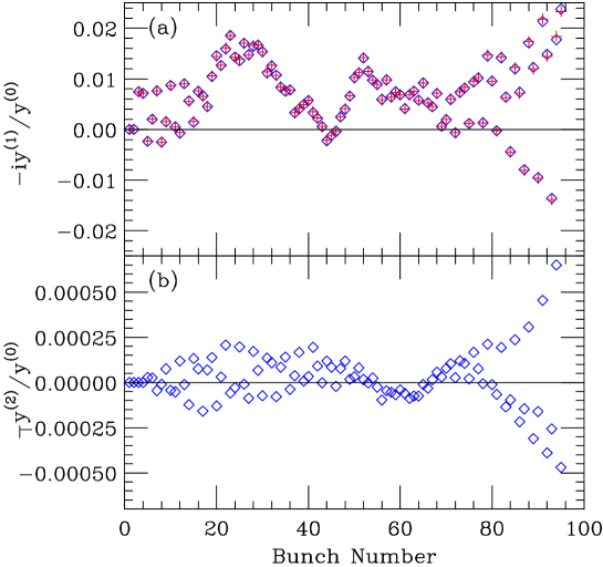
In Fig. 12 we give a numerical example: the NLC prelinac with the optimized S-band structure, but with systematic frequency errors, with the nominal (2.8 ns) bunch spacing (see the main text). The diamonds give the first order (a) and the second order (b) perturbation terms. The crosses in (a) give the results of a smooth focusing simulation program (taking ), where the free betatron term has been removed. We see that the agreement is very good; i.e. the first order term is a good approximation to the simulation results. In (b) we note that the next order term is much smaller. For this example we find that even if we increase the current by an order of magnitude the 1st order term alone remains a good approximation.
Appendix B: The Wakefield Due to Cell-to-Cell Misalignments
We assume a structure is composed of many cells that are misaligned transversely by amounts that are very small compared to the cell dimensions. For such a case we assume that the mode frequencies are the same as in the ideal structure, and only the mode kick factors are affected. To first order we assume that for each mode, the kick factor for the beam on-axis in the imperfect structure is the same as for the case with the beam following the negative of the misalignment path in the error-free structure. In Fig. 13 we sketch a portion of such a misaligned structure (top) and the model used for the kick factor calculation (bottom). The sketch is meant to represent a disk-loaded structure that has been built up from a collection of cups. Note that the relative size of the misalignements is exaggerated from what is expected, in order to more clearly show the principle. Given this model, the method of calculation of the kick factors can be derived using the so-called “Condon Method”[13],[14] (see also [15]). Note that this application to cell-to-cell misalignments in an accelerator structure is presented in Ref. [6]. The results of this perturbation method have been shown to be consistent with those using a 3-dimensional scattering matrix analysis[7]. We will only sketch the derivation below.
Consider a closed cavity with perfectly conducting walls. For such a cavity the Condon method expands the vector and scalar potentials, in the Coulomb gauge, as a sum over the empty cavity modes. As function of position and time the vector potential in the cavity is given as
| (B1) |
where
| (B2) |
with the frequency of mode , and on the metallic surface ( is a unit vector normal to the surface). Using the Coulomb gauge implies that . The are given by
| (B3) |
with the normalization
| (B4) |
with the current density. Note that the integrations are performed over the volume of the cavity .
The scalar potential is given as
| (B5) |
where
| (B6) |
with the frequencies associated with , and with on the metallic surface. The are given by
| (B7) |
with the charge distribution in the cavity. Note that one fundamental difference between the behavior of and is that when there are no charges in the cavity the vector potential can still oscillate whereas the scalar potential must be identically equal to 0.
Let us consider an ultra-relativistic driving charge that passes through the cavity parallel to the axis, and (for simplicity) a test charge following at a distance behind on the same path. Both enter the cavity at position and leave at position . The transverse wakefield at the test charge is then
| (B8) | |||||
where the integrals are along the path of the particle trajectory. The parameter is a parameter for transverse offset (the transverse wake is usually given in units of V/C per longitudinal meter per transverse meter); for a cylindrically-symmetric structure it is usually taken to be the offset, from the axis, of the driving bunch trajectory. For we can drop the scalar potential term (it must be zero when there is no charge in the cavity), and the result can be written in the form[15]
| (B9) |
with
| (B10) |
Note that the arbitrary constants associated with the parameter in the numerator and the denominator of Eq. B9 cancel. Note also that—to the same arbitrary constant— is the square of the voltage lost by the driving particle to mode and is the energy stored in mode .
Consider now the case of a cylindrically-symmetric, multi-cell accelerating cavity, and let us limit our concern to the effect of the dipole modes of such a structure. We will allow the charges to move on an arbitrary, zig-zag path in the plane that is close to the axis, and for which the slope is everywhere small (so that ). For dipole modes in a cylindrically-symmetric, multi-cell accelerator structure, it can shown that the synchronous component of (the only component that, on average, is important) can be written in the form (see e.g. Ref. [16]). Then Eq. B9 becomes
Note that this equation can be written in the form:
| (B12) |
with a kind of kick factor and the phase of excitation of mode . Note that in the special case where the particles move parallel to the axis, at offset , , the normal kick factors for the structure, and . For this case it can be shown that Eq. B12 is valid for all [15]. Finally, note that, for the general case, Eq. B12 can obviously not be extrapolated down to , since it implies that , which we believe is nonphysical, implying that a particle can kick itself transversely. To obtain the proper equation valid down to we would need to include the scalar potential term that was dropped in going from Eq. B8 to Eq. B9.
Our derivation, presented here, is technically applicable only to structures for which all modes are trapped. The modes will be trapped at least at the ends of the structure, if the connecting beam tubes have sufficiently small radii and the dipole modes do not couple to the fundamental mode couplers in the end cells. For detuned structures, like those in the injector linacs discussed in this report, most modes are trapped internally within a structure, and those that do extend to the ends couple only weakly to the beam; for such structures the results here can also be applied, even if the conditions on the beam tube radii and the fundamental mode coupler do not hold. We believe that even for the damped, detuned structures of the main linac of the JLC/NLC, which are similar, though they have manifolds to add weak damping to the wakefield, a result very similar to that presented here applies.
To estimate the wakefield associated with very small, random cell-to-cell misalignments in accelerator structures we assume that we can use the mode eigenfrequencies and eigenvectors of the error-free structure. We obtain these from the circuit program. Then to find the kick factors we replace in the first integral in Eq. Appendix B: The Wakefield Due to Cell-to-Cell Misalignments by the zig-zag path representing the negative of the cell misalignments, a path we generate using a random number generator. The normalization factor is set to the rms of the misalignments. How can we justify using this method for finding the wake at the spacing of the bunch positions? For example, for the S-band structure, the alternate bunch spacing is only 42 cm whereas the whole structure length m. Therefore, in principle, Eq. Appendix B: The Wakefield Due to Cell-to-Cell Misalignments is not valid until the 11th bunch spacing. We believe, however, that the scalar potential fields will not extend more than one or two cells behind the driving charge (the cell length is 4.375 cm), and therefore this method will be a good approximation at all bunch positions behind the driving charge. This belief should be tested in the future by repeating the calculation, but now also including the contribution from scalar potential terms.
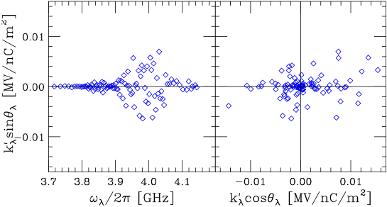
In Fig. 14 we give a numerical example. Shown, for the optimized S-band structure (see the main text), are the kick factors and the phases of the modes as calculated by the method described in this section. Note that is not necessarily small.
Appendix C: Resonant Multi-Bunch Wakefield Effects
It is easy to understand how resonances can arise in a linac with bunch trains. Consider the case of the interaction of the beam with one single structure mode. The leading bunch enters the structure offset from the axis and excites the mode. If the bunch train is sitting on an integer resonance, i.e. if , with the mode frequency, the bunch spacing, and an integer, then when the 2nd bunch arrives it will excite the mode at the same phase and also obtain a kick due to the wakefield of the first bunch. The bunch will also excite the mode in the same phase and obtain times the kick from the wakefield that the second bunch experienced (for simplicity we assume the mode is infinity). On the half-integer resonance, i.e. when , the bunch will also receive kicks from the wakefield left by the earlier bunches, but in this case the kicks will alternate in direction, and no resonance builds up. For a transverse wakefield effect, such as we are interested in, however, this simple description of the resonant interaction needs to be modified slightly. For this case the wake varies as , and neither the integer nor the half-integer resonance condition will excite any wakefield for the following bunches. In this case resonant growth is achieved at a slight deviation from the condition , as is shown below.
In the following, for simplicity, we will use the “uncoupled” model (which is described in Chapter 3 of the main text) to investigate resonant effects in the sum wake for a structure with modes with a uniform frequency distribution. The point of using the uncoupled model is that it allows us to study the effect of an idealized, uniform frequency distribution. As we have seen in the main text, an ideal (input) frequency distribution becomes distorted by the cell-to-cell coupling of an accelerator structure. As example we will use the parameters of a simplified version (all kick factors are equal) of the optimized S-band structure described in the main text; for bunch structure we consider the nominal bunch spacing ( ns). The results for the real structure, with coupled modes, will be slightly different yet qualitatively the same. Note that we are also aware of a different analysis of resonant multi-bunch wakefield effect[17].
Consider first the case of a structure with only one dipole mode, with frequency , and a kick factor that we will normalize (for simplicity) to . Suppose there are bunches in the bunch train. The sum wake at the bunch is given by
| (C1) | |||||
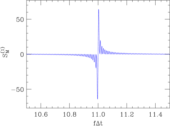
As with the nominal (2.8 ns) bunch spacing in the S-band prelinacs, let us, for an example, consider bunches and the region near the 11th harmonic. In Fig. 15 we plot vs the sum wake for the th (the last) bunch, , near the 11th integer resonance. It can be shown that, if is not small, the largest resonance peaks (the extrema of the curve) are at
| (C2) |
with values . Note that at the exact integer and half-integer resonant spacings the sum wake is zero.
Now let us consider a uniform distribution of mode frequencies. For simplicity we will let all the kick factors be equal, and be normalized to . The sum wake, according to the uncoupled model, becomes
| (C3) |
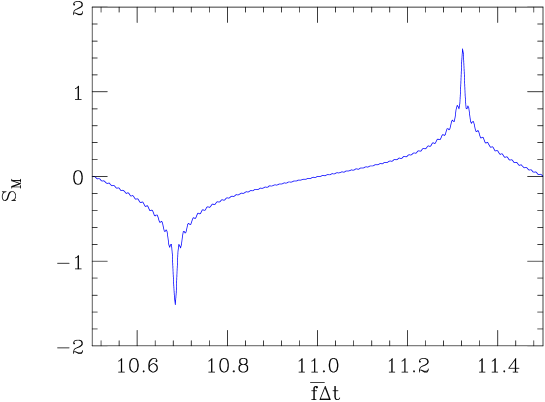
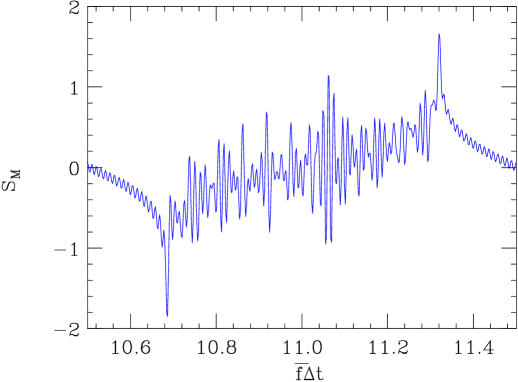
with the number of cells (also the number of modes), the central frequency, and the total (relative) width of the frequency distribution. As an example, let us consider the optimized S-band structure, with and . The sum wake at the last (the th) bunch position, , is plotted as function of in Fig. 16. Note that the uniform frequency distribution appears to suppress the integer resonance. The extrema of the curve (the “horns”) that are seen at are resonances due to the edges of the frequency distribution, with the condition . Note, however, that the sizes of even these spikes are small compared to those of the single mode case.
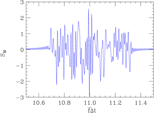
Suppose we add frequency errors to our model. We can do this by, in each term in the sum of Eq. C3, multiplying the frequency by the factor , with the rms (relative) frequency error and a random number with rms 1. Doing this, considering a uniform distribution in frequency errors with rms , Fig. 16 becomes Fig. 17. Note that this perturbation is small compared to the frequency spacing , so it does not really change the frequency distribution significantly. Nevertheless, because of resonance-like behavior we can see a large effect on throughout the range between the horns of Fig. 16 (). To model cell-to-cell misalignments, we multiply each term in the sum of Eq. C3 by the random factor . The results, for a uniform distribution of errors with rms 1, are shown in Fig. 18. Again resonance-like behavior is seen throughout the range between the horns of Fig. 16.
We can understand these results in the following manner: Only when there are no errors does using a uniform frequency distribution suppress the resonance in the region near the integer resonance. But otherwise, using a uniform frequency distribution basically only reduces the size of the resonances, at the expense of extending the range in bunch spacings where they can be excited. Instead of being localized in the region near the integer resonance (), resonance-like behavior can now be excited anywhere between the limits
| (C4) |
Note that this implies that if , then the resonance-like behavior cannot be avoided no matter what bunch spacing (fractional part) is chosen. For example, for the X-band linac in the NLC, where the total width of the dipole frequency distribution (of the dominant first band modes) is 10%, even for the alternate (1.4 ns) bunch spacing, where the integer part of is 21, the resonance region cannot be avoided.