Perturbative treatment of intercenter coupling in Redfield theory

Abstract

The quantum dynamics of coupled subsystems connected to a thermal bath is studied. In some of the earlier work the effect of intercenter coupling on the dissipative part was neglected. This is equivalent to a zeroth-order perturbative expansion of the damping term with respect to the intercenter coupling. It is shown numerically for two coupled harmonic oscillators that this treatment can lead to artifacts and a completely wrong description, for example, of a charge transfer processes even for very weak intercenter coupling. Here we perform a first-order treatment and show that these artifacts disappear. In addition, we demonstrate that the thermodynamic equilibrium population is almost reached even for strong intercenter coupling strength.

PACS: 82.30.Fi, 82.20.Wt, 82.20.Xr

I Introduction

Quantum dynamics of complex molecules or molecules in a dissipative environment has attracted a lot of attention during the last years. One special kind of this problem is the electron transfer dynamics in or between molecules especially in solution [1, 2, 3]. The bath-related relaxation can be described in a variety of ways. Among others these are the path integral methods [4, 5], the semi-group methods [6, 7, 8], and the reduced density matrix (RDM) theory [9]. The latter one has been especially successful in Redfield’s formulation [10, 11] and is the topic of the present investigation. As usual, the master equation for the RDM is derived from the equation of the full system, i.e. relevant system plus bath, by tracing out the bath degrees of freedom. The main limitations of Redfield theory are the second-order perturbation treatment in system-bath coupling and the neglect of memory effects (Markov approximation). In addition Redfield suggested the use of the secular approximation. In this approximation it is assumed that every element of the RDM in eigenstate representation (ER) is coupled only to those elements that oscillate at the same frequency. In the present study we do not perform this additional approximation which could distort the correct time evolution in transfer problems[12, 13].

To be rigorous in applying Redfield theory, the operators describing the time evolution have to be expressed in ER of the relevant system as has been done in the original papers [10, 11]. For electron transfer this was performed in part of the literature (see for example [14, 15, 16, 17]) while in another part of the literature [18, 19, 20, 21, 22, 23] diabatic (local) representations (DRs) have been used, which significantly reduces the numerical effort in many cases. In NMR literature [11, 24, 25] most people seem to use the ER while in quantum optics most people use DRs [26, 27]. Only recently the ER is used in quantum optics [28, 29, 30]. Here we focus on electron transfer systems, but the conclusions should also be applicable to problems in other areas.

While in ER the damping term is evaluated exactly, in DR the influence of the coupling between the local subsystems on dissipation is neglected. As a consequence the relaxation terms do not lead to the proper thermal equilibrium of the coupled system [31, 6, 32]. Only the thermal equilibrium of each separate subsystem is reached which can be quite different from the thermal equilibrium of the coupled system. It will be shown here that even for a very small intercenter coupling a completely wrong asymptotic value can be obtained.

Although possibly leading to the wrong thermal equilibrium the local DR has advantages. For large problems it may be difficult to calculate the eigenstates of the system. These are not necessary in the DR. There one only needs the eigenstates of the subsystems. The quantum master equation can be implemented more efficiently in DR in many cases [18, 33, 34, 35]. Moreover, almost all physical and chemical properties of transfer systems are expressed in the DR. For example, to determine the transfer rate one often calculates the population of the diabatic states and obtains the rate from their time evolution. To do so one has to switch back and forth between DR and ER all the time if the time evolution is determined in ER.

Using the semi-group methodology and a simple model of two fermion sites, DR and ER have been compared already [6]. We are interested in a more complicated system, i.e. a curve-crossing problem. The fact that we use a different relaxation mechanism should effect the findings only very little. Here we not only compare DR and ER but show how the relaxation term in DR can be written more precisely for small intercenter coupling.

The paper is organized as follows. The next section gives an introduction to the Redfield theory and, using the DR, presents a zeroth-order (DR0) and a first-order (DR1) perturbation expansion in the intercenter coupling. In the third section numerical examples are shown for two coupled harmonic oscillators. The DR and ER results are compared to each other and also to the improved local relaxation term derived here. The last section gives a short summary. Atomic units are used unless otherwise stated.

II Intercenter perturbation expansion within the Redfield equation

In the RDM theory the full system is divided into a relevant system part and a heat bath. Therefore the total Hamiltonian consists of three terms – the system part $H_{\rm S}$, the bath part $H_{\rm B}$, and the system-bath interaction $H_{\rm SB}$:

$$H=H_{\rm S}+H_{\rm B}+H_{\rm SB}.$$ (1)

The RDM $\rho$ is obtained from the density matrix of the full system by tracing out the degrees of freedom of the environment. This reduction together with a second-order perturbative treatment of $H_{\rm SB}$ and the Markov approximation leads to the Redfield equation [10, 11, 9, 36]:

$$\dot{\rho}=-i[H_{\rm S},\rho]+{\cal R}\rho={\cal L}\rho.$$ (2)

In this equation ${\cal R}$ denotes the Redfield tensor. If one assumes bilinear system-bath coupling with system part $K$ and bath part $\Phi$

$$H_{\rm SB}=K\Phi$$ (3)

one can take advantage of the following decomposition [37, 36]:

$$\dot{\rho}=-i\left[H_{\rm S},\rho\right]+\{[\Lambda\rho,K]+[K,\rho\Lambda^{\dagger}]\}.$$ (4)

Here $K$ and $\Lambda$ together hold the same information as the Redfield tensor ${\cal R}$. The $\Lambda$ operator can be written in the form

$$\Lambda=\int\limits_{0}^{\infty}d\tau\langle\Phi(\tau)\Phi(0)\rangle K^{\rm{I}}(-\tau)$$ (5)

where $K^{\rm{I}}(-\tau)=e^{-iHt}Ke^{iHt}$ is the operator $K$ in the interaction representation. Assuming a quantum bath consisting of harmonic oscillators the time correlation function of the bath operator is given as [15]

$$C(\tau)=\langle\Phi(\tau)\Phi(0)\rangle=\int\limits_{0}^{\infty}d\omega J(\omega)n(\omega)(e^{i\omega t}+e^{\beta\omega}e^{-i\omega t})~{}.$$ (6)

Here $J(\omega)$ denotes the spectral density of the bath [15], $n(\omega)=(e^{\beta\omega}-1)^{-1}$ the Bose-Einstein distribution, and $\beta=1/(k_{\rm B}T)$ the inverse temperature.

The Hamiltonian $H_{\rm S}$ of the system we are interested in can be separated according to

$$H_{\rm S}=H_{0}+V$$ (7)

where $H_{0}$ is the sum of all uncoupled subsystem Hamiltonians $H_{0,n}$

$$H_{0}=\sum_{n}H_{0,n}$$ (8)

and $V$ the coupling among them which is assumed to be small. Two canonical bases can be constructed for such a Hamiltonian. One consists of eigenfunctions of $H_{0}$. It is often called a local basis because these basis functions of the diabatic potential energy surfaces (PESs) are located at specific subsystems (centers). Latin indices such as $|n\rangle$ are used below to denote these DR basis states. The other basis diagonalizes the system Hamiltonian $H_{\rm S}$. So it consists of eigenstates of $H_{\rm S}$ and is called adiabatic basis. For these ER basis functions we use Greek indices such as $|\nu\rangle$. As discussed in the introduction Redfield theory is defined in ER but for transfer problems DRs have some conceptual and numerical advantages.

Here we first calculate the dissipation in the DR for small intercenter coupling $V$. In this basis the matrix elements of $\Lambda$ are given by

$$\langle n|\Lambda|m\rangle=\int\limits_{0}^{\infty}d\omega J(\omega)n(\omega)\int\limits_{0}^{\infty}d\tau(e^{i\omega\tau}+e^{\beta\omega}e^{-i\omega\tau})\langle n|K^{\rm I}(-\tau)|m\rangle~{}.$$ (9)

To evaluate the matrix element of $K$ one has to use perturbation theory in $V$ because the diabatic states $|n\rangle$ are not eigenstates of $H_{\rm S}$ but of $H_{0}$. Some details of the determination of $\langle n|\Lambda|m\rangle$ are given in the appendix. Using the expression for the correlation function in frequency space

$$C(\omega)=2\pi[1+n(\omega)][J(\omega)-J(-\omega)]~{},$$ (10)

and denoting the transition frequency between diabatic states $|m\rangle$ and $|n\rangle$ by $\omega_{mn}$ the final result can be written as

$$\langle n|\Lambda|m\rangle = \frac{1}{2}C(\omega_{mn})\langle n|K|m\rangle$$ (13)

$$-\frac{1}{2}\sum_{j}\langle n|K|j\rangle\frac{\langle j|V|m\rangle}{\omega_{jm}}\left[C(\omega_{mn})-C(\omega_{jn})\right]$$

$$-\frac{1}{2}\sum_{i}\langle i|K|m\rangle\frac{\langle n|V|i\rangle}{\omega_{ni}}\left[C(\omega_{mn})-C(\omega_{mi})\right]~{}.$$

This first-order result DR1 can be split into a zeroth-order contribution DR0 independent of $V$ and a first-order contribution proportional to $V$. Taking the DR0 term

$$\langle n|\Lambda|m\rangle = \frac{1}{2}C(\omega_{mn})\langle n|K|m\rangle$$ (14)

only is equivalent to a complete neglect of the influence of the intercenter coupling $V$ on dissipation. This assumption has been used earlier [18, 19, 20, 21, 22, 23] and is sometimes called the diabatic damping approximation [38]. In this approximation only the states $|n\rangle$ and $|m\rangle$ contribute to the matrix element $\langle n|\Lambda|m\rangle$. In DR1 all states contribute to each of these matrix elements. As a consequence the spectral density of the bath is not only probed at the transitions of the uncoupled subsystems as in DR0 but at many more frequencies.

The ER result for the matrix elements of $\Lambda$ can easily be deduced from the DR result by replacing the diabatic states by adiabatic ones and setting $V=0$ in Eq. (13):

$$\langle\nu|\Lambda|\mu{}\rangle = \frac{1}{2}C(\omega_{\mu{}\nu})\langle\nu|K|\mu{}\rangle~{}.$$ (15)

This result is of course correct for arbitrary intercenter coupling strength.

III Electron transfer in a two-center system

In the following we direct our attention to electron transfer in an example system consisting of two charge localization centers considered to be excited electronic states. The PESs of the localization centers are assumed to be harmonic and are sketched in Fig. 1. For this example the Hamiltonian of the uncoupled system is given by

$$H_{0}=\sum_{n}\left[U_{n}+\left(a_{n}^{\dagger}a_{n}+\frac{1}{2}\right)\omega_{n}\right]$$ (16)

and the coupling by

$$V=\sum_{m,n}\sum_{M,N}(1-\delta_{mn})v_{mn}|mM\rangle\langle nN|~{}.$$ (17)

The first index in each vector denotes the diabatic PES while the second labels the vibrational level. $a_{n}$ and $a_{n}^{\dagger}$ are the boson operators for the normal modes at center $n$ and $\omega_{n}$ are the eigenfrequencies of the oscillators. Bilinear system-bath coupling is assumed and the system part is given by the coordinate operator $q$

$$K=q=\sum\limits_{m}\sum_{MN}\left(2\omega_{m}{\cal M}\right)^{-1/2}\left(a_{m}^{\dagger}+a_{m}\right)|mM\rangle\langle mN|~{}$$ (18)

The mass of the system is denoted by ${\cal M}$.

In the local DR the system part of the system-bath coupling reads

$$\langle mM|K|nN\rangle=\left(2\omega_{m}{\cal M}\right)^{-1/2}\delta_{mn}\left(\delta_{M+1,N}\sqrt{M+1}+\delta_{M-1,N}\sqrt{M}\right)~{}.$$ (19)

In the DR0 expansion (14) the system can emit or absorb only at intra-subsystem transition frequencies $\omega_{MN}$. The spectral density of the bath $J(\omega)$ is effectively reduced to discrete values $J(\omega)=\sum_{m}\gamma_{m}\delta(\omega-\omega_{m})$. The advantage of this approach is the scaling behavior of the CPU time with the number ${\cal N}$ of basis functions which results from the simple structure of the $\Lambda$ matrix (14). As shown numerically [35, 34] it scales like ${\cal N}^{2.3}$. This is far better than the ${\cal N}^{3}$ scaling of the DR1 approximation (13). In DR1 the spectral density is probed at many more frequencies. One needs the full frequency dependence of $J(\omega)$ which we take to be of Ohmic form with exponential cut-off

$$J(\omega)=\eta\Theta(\omega)\omega e^{-\omega/\omega_{c}}.$$ (20)

Here $\Theta$ denotes the step function and $\omega_{c}$ the cut-off frequency. In this study all system oscillators have the same frequency $\omega_{1}$ (see Table I) and the cut-off frequency $\omega_{c}$ is set equal to $\omega_{1}$. The normalization prefactor $\eta$ is determined such that the spectral densities in DR and ER coincide at $\omega_{1}$. Eq. (20) together with Eq. (10) yields the full correlation function.

If the system Hamiltonian $H_{\rm S}$ is diagonalized and the resulting ER basis is used to calculate the elements of the operators in Eq. (4), there will be no longer any convenient structure in $K$ or $\Lambda$, so that the full matrix-matrix multiplications are inevitable. For this reason the CPU time scales as ${\cal N}^{3}$, where ${\cal N}$ is the number of eigenstates of $H_{\rm S}$. There appears to be a minimal number ${\cal N}_{0}$ below which the diagonalization of $H_{\rm S}$ fails or the completeness relation for $|\nu\rangle$ is violated. Nevertheless, the benefit of this choice is the exact treatment of the intercenter coupling. It is straightforward to obtain the matrices for $\rho$ and $K$ (see for example Ref. [14]).

An initial wave packet at center $|n\rangle$ is prepared by a $\delta$-pulse excitation from the ground state $|{\rm g}\rangle$ of the system

$$\rho_{1M1N}(t=0)=\langle 1M|{\rm g}0\rangle\langle{\rm g}0|1N\rangle~{}.$$ (21)

The pulse is chosen such that mainly the fourth and fifth vibrational level of the first (left) diabatic PES is populated. The motion of the initial wave packet along the coordinate $q$ models the transfer between the centers. The parameters for our calculation are taken from the work of Kühn et al. [20] and are shown in Table I. Temperature is chosen as $T=295$ K and the reduced mass of the system ${\cal M}$ is set to 20 proton masses. The RDM is propagated in time and the occupation probabilities for each localization center are calculated by means of the partial trace:

$$P_{m}=\sum\limits_{M}\rho_{mMmM}.$$ (22)

For the case of propagating in ER the RDM is transformed back to the DR in order to apply Eq. (22).

In the following we compare the population dynamics in the two-center electron transfer system using three different intercenter coupling strengths $V$ and four different configurations of the two harmonic PESs. The diabatic PESs and eigenenergies are shown in Fig. 1. Beginning our analysis with the weak coupling case $v=v_{12}=v_{21}=0.1\omega_{1}$ it is expected that a perturbation expansion in $V$ yields almost exact results. This is the reasoning why the DR0 term, which is easy to implement, has been used in earlier work [18, 19, 20, 21, 22, 23].

In configuration (a) the eigenenergies of the two diabatic PESs are in resonance. For example, the first vibrational eigenenergy of the first center equals the third vibrational eigenenergy of the second center. It is important to note that in this configuration no vibrational level of the first center is below the crossing point of the two PESs. The calculations using ER and DR0 as well as DR1 give almost identical results, see Fig. 2a. For long times DR0 deviates a tiny bit. Redfield theory in ER is known to give the correct long-time limit (up to the Lamb shift).

Configuration (b) differs from the first one by shifting the first PES up by $\omega_{1}/2$. As shown in Fig. 2b the ER and DR1 results again agree perfectly. On the other hand, the DR0 results are a little bit off already at early times and the equilibrium value departs from the correct value much more than in the first, on-resonance configuration.

Shifting the PESs further apart than in (a) yields configuration (c). The energy levels are again on-resonance but this time two vibrational levels of the first center are below the curve-crossing point, i.e. there is a barrier for low-energy parts of the wave packet. As shown in Fig. 2c DR1 and the ER results agree perfectly once more. The DR0 results are terribly off. The long-time population of the first center which should vanish for the present configuration stays finite.

If we increase the energy of the first PES by $\omega_{1}/2$ to obtain configuration (d) DR0 fails again while DR1 gives correct results in comparison to the ER, see Fig. 2d.

To understand the large difference between DR0 and DR1 we have a closer look at the final result for the matrix elements of $\Lambda$, Eqs. (13) and (14). The DR0 contribution (14) is independent of the intercenter coupling $V$. The system part of the system-bath interaction $K$ allows only for relaxation within each center. So there is no mechanism in the dissipative part which transfers population from one center to the other. This transfer has to be done by the coherent part of the master equation. But the coherent part cannot transfer components of the wave packet with energy below the crossing point of the PESs. As tunneling is mainly suppressed, those components of the wave packet cannot leave their center anymore although the corresponding PES might be quite high in energy. This results in the failure of DR0 for the configurations with barrier: Parts of the wave packet get trapped in the two lowest levels of the left center. From Eq. (13) one can explain why in the on-resonance case the DR0 results are in better agreement with the correct results. In this configuration some of the DR1 terms are very small and so the DR1 correction is smaller.

Now we discuss the medium coupling strength $v=0.5\omega_{1}$ (see Fig. 3). The results for configurations (a) and (b), i.e. without barrier, look quite similar. In both cases the ER and DR1 results agree very well for short and long times. At intermediate times there is a small difference. The DR0 results already deviate at short times and for long times there is too much population in the left (higher) center. For configurations (c) and (d), i.e. with barrier, again the ER and DR1 results coincide for small and long times. DR0 is off already after rather short times and the long-time limit is again wrong.

For the strong coupling $v=\omega_{1}$ (see Fig. 4) the behavior of the results is quite similar to the medium coupling. For configurations (a) and (b) the difference at intermediate times is a little larger, so is the deviation of the long-time DR0 limit. For configurations (c) and (d) with barrier there is also a discrepancy for DR1 already at short times and the correct long-time limit is not reached exactly. But the disagreement is surprisingly small for the strong coupling. Overall DR1 still looks quite reasonable while the DR0 results are completely off.

IV Summary

In addition to the approximations done in Redfield theory, i.e. second-order perturbation expansion in the system-bath coupling and Markov approximation, we have applied perturbation theory in the intercenter coupling. It has been shown for two coupled harmonic surfaces that the zeroth-order approximation DR0 which is equivalent to the diabatic damping approximation [38] can yield wrong population dynamics even for very small intercenter coupling. These artifacts disappear using the first-order theory DR1.

The scaling of DR1 is like ${\cal N}^{3}$ not as ${\cal N}^{2.3}$ for DR0. This is of course a serious drawback of DR1. For configurations without barrier it seems to be possible to use DR0 for weak to medium intercenter coupling. This of course depends on the accuracy required especially for the long-time limit. In all other cases one should either use the exact ER or DR1. Although the first-order results are not exact for medium and strong intercenter coupling these calculations have at least two advantages. First of all, one does not need to calculate the eigenstates and energies of the full system Hamiltonian $H_{\rm S}$. For small systems like two coupled harmonic surfaces using one reaction coordinate this calculation is of course easy. But if one wants to study larger systems like molecular wires [6, 14] and/or multi-mode models [22, 23, 33] this is no longer a trivial task. The second advantage is related to the fact that in all transfer problems one is mainly interested in properties which are defined in a local basis, e. g. the population in each subsystem in any moment in time. If one uses the ER one has always to transform back to the DR in order to calculate these properties. So for large-scale problems using a DR together with the first-order perturbation in $V$ should be advantageous.

In a sense the present study is an extension of the investigation performed by Davis et al. [6]. They compared ER and DR for a two-site problem. Here we looked at a more general multilevel system and also calculated the first-order perturbation. In their model they do not have a reaction coordinate and therefore no barrier. Their findings correspond more to cases (a) and (b) in the previous section. Besides the agreement in the case of small intercenter coupling they also found good agreement in the high-temperature limit. Using our model this statement could not be confirmed for a general configuration, although there might be configurations where it is true.

In Ref. [30] the authors followed a strategy different from the present work. They also studied two coupled harmonic oscillators modeling two coupled microcavities, but only one cavity was coupled to the thermal bath directly. This should not effect the questions studied here. With a transformation to uncoupled oscillators they effectively reduced the intercenter coupling to zero. The result [30] is then exact for arbitrary $V$. The disadvantage of this strategy is that it is not easy to extend to larger systems. The advantage of the presently developed first-order expansion in $V$ is its general applicability to problems of any size.

The purpose of this appendix is to show some more details for the evaluation of $\langle n|\Lambda|m\rangle$. To calculate

$$\langle n|K^{\rm I}(-t)|m\rangle = \sum_{i,j}\langle n|e^{-iHt}|i\rangle\langle i|K|j\rangle\langle j|e^{iHt}|m\rangle$$ (23)

the operator identity [39]

$$e^{-i(H_{0}+V)t}=e^{-iH_{0}t}\left(1-i\int\limits_{0}^{t}dt^{\prime}e^{it^{\prime}H_{0}}Ve^{-it^{\prime}(H_{0}+V)}\right)~{},$$ (24)

which can easily be proven by multiplying both sides by $e^{iH_{0}t}$ and differentiating with respect to $t$, is used iteratively. It yields

$$\langle n|e^{-iHt}|i\rangle = \langle n|e^{-iH_{0}t}[1-i\int\limits_{0}^{t}dt^{\prime}e^{it^{\prime}H_{0}}Ve^{-it^{\prime}H_{0}}]|i\rangle+{\cal O}(V^{2})$$ (25)

$$= e^{-iE_{i}t}\delta_{ni}-ie^{-iE_{n}t}\langle n|V|i\rangle\int\limits_{0}^{t}dt^{\prime}e^{i(E_{n}-E_{i})t^{\prime}}+{\cal O}(V^{2})$$ (26)

$$= e^{-iE_{i}t}\delta_{ni}-\frac{\langle n|V|i\rangle}{E_{n}-E_{i}}(e^{-iE_{i}t}-e^{-iE_{n}t})+{\cal O}(V^{2})$$ (27)

assuming that $E_{n}\neq E_{i}$. Here and in the following we only give the general expressions for the matrix elements. If a singularity can appear due to coinciding frequencies the appropriate expression can be obtained by taking the proper limit.

Thus the matrix element (23) is given by

$$\langle n|K^{\rm I}(-t)|m\rangle = e^{i\omega_{mn}t}\langle n|K|m\rangle$$ (30)

$$-\sum_{j}\langle n|K|j\rangle\frac{\langle j|V|m\rangle}{\omega_{jm}}(e^{i\omega_{mn}t}-e^{i\omega_{jn}t})$$

$$-\sum_{i}\langle i|K|m\rangle\frac{\langle n|V|i\rangle}{\omega_{ni}}(e^{i\omega_{mi}t}-e^{i\omega_{mn}t})+{\cal O}(V^{2})$$

This result is inserted into Eq. (9). One has to evaluate integrals of the kind

$$\int\limits_{0}^{\infty}dte^{-\epsilon t}e^{-i\omega_{mn}t}=\frac{-i}{\omega-\omega_{nm}-i\epsilon}$$ (31)

which contain a convergence parameter $\epsilon$. Using the well known identity

$$\lim_{\epsilon\to 0}\frac{1}{x\pm{}i\epsilon}=\frac{P}{x}\mp\pi\delta(x)$$ (32)

one gets for the first term of the matrix element of $\Lambda$

$$\langle n|\Lambda|m\rangle = \frac{\pi}{1-e^{-\beta\omega_{mn}}}[J(\omega_{mn})-J(-\omega_{mn})]\langle n|K|m\rangle+({\rm Lamb}~{}{\rm shift})+\ldots$$ (33)

The Lamb shift is the imaginary part of the matrix element of $\Lambda$ and leads to an energy shift in the quantum master equation. This term is a small correction [40, 41] and is neglected in Redfield theory. The other terms of the matrix elements are calculated in the same fashion yielding

$$\langle n|\Lambda|m\rangle = \frac{\pi}{1-e^{-\beta\omega_{mn}}}[J(\omega_{mn})-J(-\omega_{mn})]\langle n|K|m\rangle$$ (38)

$$-\sum_{j}\langle n|K|j\rangle\frac{\langle j|V|m\rangle}{\omega_{jm}}\left\{\frac{\pi}{1-e^{-\beta\omega_{mn}}}[J(\omega_{mn})-J(-\omega_{mn})]\right.$$

$$\left.-\frac{\pi}{1-e^{-\beta\omega_{jn}}}[J(\omega_{jn})-J(-\omega_{jn})]\right\}$$

$$-\sum_{i}\langle i|K|m\rangle\frac{\langle n|V|i\rangle}{\omega_{ni}}\left\{\frac{\pi}{1-e^{-\beta\omega_{mn}}}[J(\omega_{mn})-J(-\omega_{mn})]\right.$$

$$\left.-\frac{\pi}{1-e^{-\beta\omega_{mi}}}[J(\omega_{mi})-J(-\omega_{mi})]\right\}$$

TABLE I.: Parameters used for the ground state oscillator and the two excited state oscillators.

Center $|n\rangle$	Configuration	$U_{n}$, eV	$Q_{n}$, ${\rm\AA{}}$	$\omega_{n}$, eV
$|{\rm g}\rangle$		0.00	0.000	0.1
$|1\rangle$		0.25	0.125	0.1
$|2\rangle$	a	0.05	0.238	0.1
$|2\rangle$	b	0.00	0.238	0.1
$|2\rangle$	c	0.05	0.363	0.1
$|2\rangle$	d	0.00	0.363	0.1

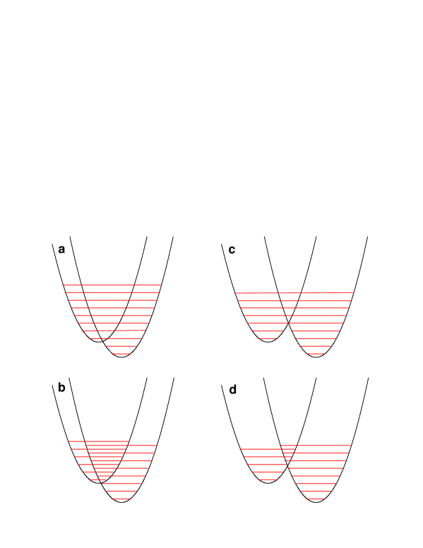
FIG. 1.: The four different configurations of the two diabatic harmonic potentials $|1\rangle$ and $|2\rangle$ as discussed in the text. Also included in the figures are the energy levels.

FIG. 2.: Time evolution for small intercenter coupling and for the four different configurations. The results in ER are shown by the solid line while the results in diabatic basis are shown by dotted (zeroth-order) and dashed (first-order) lines. The results for ER and DR1 are indistinguishable for small intercenter coupling. Note the logarithmic time scale.

FIG. 3.: Time evolution for medium intercenter coupling.

FIG. 4.: Time evolution for strong intercenter coupling.

REFERENCES

- [1] M. Bixon and J. Jortner, Adv. Chem. Phys. 106&107, (1999), special issue on electron transfer.
- [2] M. Newton, Chem. Rev. 91, 767 (1991).
- [3] P. F. Barbara, T. J. Meyer, and M. A. Ratner, J. Phys. Chem. 100, 13148 (1996).
- [4] U. Weiss, Quantum Dissipative Systems, 2nd ed. (World Scientific, Singapore, 1999).
- [5] N. Makri, J. Phys. Chem. A 102, 4414 (1998).
- [6] W. B. Davis, M. R. Wasielewski, R. Kosloff, and M. A. Ratner, J. Phys. Chem. A 102, 9360 (1998).
- [7] R. Kosloff, M. A. Ratner, and W. W. Davis, J. Chem. Phys. 106, 7036 (1997).
- [8] D. Kohen, C. C. Marston, and D. J. Tannor, J. Chem. Phys. 107, 5236 (1997).
- [9] K. Blum, Density Matrix Theory and Applications, 2nd ed. (Plenum Press, New York, 1996).
- [10] A. G. Redfield, IBM J. Res. Dev. 1, 19 (1957).
- [11] A. G. Redfield, Adv. Magn. Reson. 1, 1 (1965).
- [12] I. Barvik, V. Čápek, and P. Heřman, J. Lumin. 83-84, 105 (1999).
- [13] I. Barvik and J. Macek, J. Chin. Chem. Soc. 47, 647 (2000).
- [14] A. K. Felts, W. T. Pollard, and R. A. Friesner, J. Phys. Chem. 99, 2029 (1995).
- [15] W. T. Pollard, A. K. Felts, and R. A. Friesner, Adv. Chem. Phys. 93, 77 (1996).
- [16] J. M. Jean, J. Chem. Phys. 104, 5638 (1996).
- [17] J. M. Jean, J. Phys. Chem. A 102, 7549 (1998).
- [18] V. May and M. Schreiber, Phys. Rev. A 45, 2868 (1992).
- [19] V. May, O. Kühn, and M. Schreiber, J. Phys. Chem. 97, 12591 (1993).
- [20] O. Kühn, V. May, and M. Schreiber, J. Chem. Phys. 101, 10404 (1994).
- [21] C. Fuchs and M. Schreiber, J. Chem. Phys. 105, 1023 (1996).
- [22] B. Wolfseder and W. Domcke, Chem. Phys. Lett. 235, 370 (1995).
- [23] B. Wolfseder and W. Domcke, Chem. Phys. Lett. 259, 113 (1996).
- [24] J. Jeener, A. Vlassenbroek, and P. Broekaert, J. Chem. Phys. 103, 1309 (1995).
- [25] M. Cuperlovic, G. H. Meresi, W. E. Palke, and J. T. Gerig, J. Magn. Reson. 142, 11 (2000).
- [26] C. Cohen-Tannoudji, J. Dupont-Roc, and G. Grynberg, Atom-Photon Interactions (Wiley, New York, 1992).
- [27] B. W. Shore and P. L. Knight, J. Mod. Opt. 40, 1195 (1993).
- [28] J. D. Cresser, J. Mod. Opt. 39, 2187 (1992).
- [29] M. Murao and F. Shibata, Physica A 217, 348 (1995).
- [30] H. Zoubi, M. Orenstien, and A. Ron, Phys. Rev. A 62, 033801 (2000).
- [31] R. A. Harris and R. Silbey, J. Chem. Phys. 83, 1069 (1985).
- [32] D. Segal, A. Nitzan, W. B. Davis, M. R. Wasielewski, and M. A. Ratner, J. Phys. Chem. B 104, 3817 (2000).
- [33] B. Wolfseder, L. Seidner, W. Domcke, G. Stock, M. Seel, S. Engleitner, and W. Zinth, Chem. Phys. 233, 323 (1998).
- [34] M. Schreiber, I. Kondov, and U. Kleinekathöfer, J. Mol. Liq. 86, 77 (2000).
- [35] I. Kondov, U. Kleinekathöfer, and M. Schreiber, J. Chem. Phys. (in press) (2001).
- [36] V. May and O. Kühn, Charge and Energy Transfer in Molecular Systems (Wiley-VCH, Berlin, 2000).
- [37] W. T. Pollard and R. A. Friesner, J. Chem. Phys. 100, 5054 (1994).
- [38] D. Egorova and W. Domcke, private communication.
- [39] B. B. Laird, J. Budimir, and J. L. Skinner, J. Chem. Phys. 94, 4391 (1991).
- [40] V. Romero-Rochin and I. Oppenheim, Physica A 155, 52 (1989).
- [41] E. Geva, E. Rosenman, and D. J. Tannor, J. Chem. Phys. 113, 1380 (2000).