Atomic Energy Levels with QED
and Contribution of the Screened Self-Energy

Éric-Olivier Le Bigot, Paul Indelicato

Abstract

We present an introduction to the principles behind atomic energy level calculations with Quantum Electrodynamics (QED) and the two-time Green’s function method; this method allows one to calculate an effective Hamiltonian that contains all QED effects and that can be used to predict QED Lamb shifts of degenerate, quasidegenerate and isolated atomic levels.

Introduction

This contribution is concerned with the evaluation of atomic energy levels with QED. Such an evaluation yields stringent tests of QED in strong electric fields, whereas $g$ -factor experiments and calculations currently probe QED in situations where the magnetic field can be treated perturbatively

The nuclear Coulomb field experienced by the inner levels of highly-charged ions makes the electrons reach relativistic velocities. Such simple physical systems are thus particularly interesting for testing relativistic effects in quantum systems (for example, see Refs. [1, 2] for experimental results with lithiumlike ions). Theoretical predictions of energy levels in such systems obviously require the use of QED.

Experiments have reached an accuracy that shows that extremely accurate evaluations of QED effects are also needed in helium. Experiments performed during the last ten years in the spectroscopy of this atom have become two orders of magnitude more precise than the current theoretical calculations (see for instance Refs. [3, 4] and references therein).

Several experiments are now focusing on helium and heliumlike ions, and especially their $1s2p\,^{3}\!P_{J}$ fine structure [5, 6, 7, 8] such experiments have implications in metrology, as they could provide a measurement the fine structure constant and provide checks of theoretical higher-order effects. Very precise theoretical calculations of energy levels in heliumlike ions can be also important in the investigation of parity violation [9].

Predictions of energy levels are usually more difficult to obtain for states with one or more open shells (retardation in the interaction and exchange of electrons must be included, and there can be quasidegenerate levels). Only a few calculations of excited energy levels in heliumlike and lithiumlike ions have been performed up to now; the first results have been published quite recently [10, 11, 12]. In regards to QED shifts of quasidegenerate levels, they have only been obtained this year for the first time [11], with the help of the method that we present in this talk.

Theoretical methods

As is well known, relativistic electrons orbiting a nucleus are well treated with the Dirac equation, in which the nucleus can be considered as point-like or not. We thus treat the binding to the nucleus non-perturbatively by using “Bound-State QED” [13, 14] (the coupling constant of the nucleus-electron interaction is $Z\alpha$ , which is not small for highly-charged ions). In this formalism, however, QED effects are taken into account by treating the electron-electron interaction perturbatively (with coupling constant $\alpha$ ), and both the electron and photon fields are quantum fields (i.e., in second-quantized form); the only difference with the free-field case used in high-energy physics is that electronic creation and annihilation operators create and destroy atomic states instead of free particles.

A few methods allow one to extract energy levels from the Bound-State QED Hamiltonian: the two-time Green’s function method [15, 16, 17], the method being developed by Lindgren (based on Relativistic Many-Body Perturbation Theory merged with QED) [18, 19], the adiabatic $S$ -matrix formalism of Gell-Mann, Low and Sucher [20], and the evolution operator method [21, 22]. Some other methods yield atomic energy levels, but they include QED effects only partly or approximately (such as the multiconfiguration Dirac-Fock method [23], configuration interaction calculations [24] and relativistic many-body perturbation theory [25]).

However, only two methods can in principle be employed in order to calculate energy levels of quasidegenerate atomic states [e.g., the $(2s2p_{1/2})_{1}$ and the $(2s2p_{3/2})_{1}$ levels in heliumlike ions, which are experimentally important]: the two-time Green’s function method and the method being elaborated by Lindgren. We present in this talk a non-technical introduction to the first method. The two-time Green’s function method has also the advantage of yielding a simpler renormalization procedure than the Gell-Mann–Low–Sucher method in the case of degenerate levels [26, 27].

The two-time Green’s function method

All the methods that extract atomic energy levels from the Bound-State QED Hamiltonian study the propagation of electrons between two different times. The methods differ in the number of infinite times used:

(a) in the Gell-Mann–Low–Sucher method, the atomic state under consideration evolves from time $-\infty$ to time $+\infty$ with an adiabatic switching of the interaction; (b) in Lindgren’s formalism [18, 19], the evolution is from time $-\infty$ to time $0$ , which avoids problems associated with the two infinite times in the $S$ -matrix approach of Gell-Mann–Low–Sucher; (c) in the two-time Green’s function method, that we present here, the adiabatic switching is completely avoided by studying the propagation of electrons between two finite times. We note that adiabatic switching of the interactions is physically motivated in the study of collisions between particles that start very far from each other, but this switching is not so easily related to the physical description of the orbiting electrons of an atom.

The Green’s function

Refer to caption — FIG. 1.: The two-time Green’s function represents the probability amplitude for going from one position of the electrons to another position.

The effective Hamiltonian derived from QED by the two-time Green’s function method has matrix elements between the various degenerate and/or quasidegenerate states under study; the eigenvalues of this Hamiltonian are the atomic energy levels predicted by QED (to a given order). This effective Hamiltonian is however not associated to a Schrödinger equation of motion; our Hamiltonian is equivalent to the submatrix used in the perturbation theory of degenerate and quasidegenerate states; in this respect, the approach of the two-time Green’s function method differs from the spirit of the Bethe-Salpeter equation.

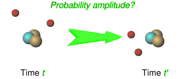
The QED Hamiltonian of the method is defined with the help of a Green’s function that represents the propagation of $N$ electrons between two different (finite) times ( $N$ is the number of electrons of the atom or ion that we want to study); this propagation is represented in Fig. 1.

Atomic energies are in the Green’s function

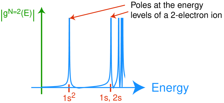
The energy levels of an $N$ -electron ion or atom can be recovered by studying the energy representation ${\mathcal{G}}^{N}(E)$ of the Green’s function, i.e., by doing a Fourier transform: this function has (simple) poles at the atomic energy levels [15, 16, 17]. Such a result is similar to the Källén-Lehmann representation [28]. As an example, Fig. 2 depicts the poles of the two-particle Green’s function.

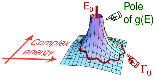
The two-time Green’s function method provides a way of mathematically extracting from the Green’s function the positions of the poles, i.e., the atomic energy levels [17]; the procedure handles degenerate and quasidegenerate atomic levels without any special difficulty [29]. One of the basic ideas behind the pole extraction is found in the following mathematical device, which uses any contour $\Gamma_{0}$ that encloses the pole in order to find its exact position: if the function $g(E)$ has a simple pole at $E=E_{0}$ , then we have from complex analysis

E_{0}=\frac{\displaystyle{\displaystyle\oint_{\Gamma_{0}}\!}d{E}\,E\times g(E)}{{\displaystyle\oint_{\Gamma_{0}}\!}d{E}\,g(E)};

(1)

the contour $\Gamma_{0}$ is only required to encircle the pole and to be positively oriented, as shown in Fig. 3. Since the Green’s function has simple poles at the atomic energy levels [17], Eq. (1) is a way of obtaining them.

When QED shifts of degenerate of quasidegenerate levels are calculated, the scalar Green’s function $g$ of Eq. (1) is simply replaced by a finite-size matrix defined on the space of levels under consideration [29].

Graphical calculations

Obviously, analytic properties of the Green’s function [27] are important in the evaluation of Eq. (1). We have developed a set of graphical techniques that allow one to obtain the Laurent series of the Green’s function ${\mathcal{G}}^{N}(E)$ by a systematic procedure. The idea behind these techniques consists in displaying the analytic structure of the Green’s function step by step; each step explicitly extracts one singularity, and we proceed until we have exhausted all the singularities of the Green’s function; at this point, contour integrals such as Eq. (1) can be calculated quite simply.

It is impossible to give here a full account of the method we use for deriving the effective, finite-size QED Hamiltonian. However, we can mention a particular feature of our calculational strategy: a very special “particle” appears in our algorithm; this particle is quite simple since it “disintegrates” immediately (zero life time) and cannot move (zero probability for going from one position to a different one). In mathematical terms, the coordinate-space propagator of this particle is a four-dimensional Delta function $\delta^{(4)}[(\vec{x},t);(\vec{x^{\prime}},t^{\prime})]$ that we represent by a special line in Feynman diagrams.

The screened self-energy

The experimental accuracy on transition energies is so high that second-order (i.e., two-photon) effects must be taken into account in order to compare experiments with theory. We thus have very recently calculated the contribution of the self-energy screening [30] to the QED effective hamiltonian; this contribution corresponds to the following physical processes:

Our result is part of the current theoretical effort developed with the aim of matching experimental precisions.

REFERENCES

[1] Beiersdorfer, P., Osterheld, A. L., Scofield, J. H., López-Urrutia, J. R. C., and Widmann, K., Phys. Rev. Lett. 80, 3022–3025 (1998).
[2] Schweppe, J., Belkacem, A., Blumenfeld, L., Claytor, N., Feynberg, B., Gould, H., Kostroun, V., Levy, L., Misawa, S., Mowat, R., and Prior, M., Phys. Rev. Lett. 66, 1434–1437 (1991).
[3] Drake, G. W. F. and Martin, W. C., Can. J. Phys. 76, 679–698 (1998).
[4] Drake, G. W. F. and Goldman, S. P., Can. J. Phys. 77, 835–845 (2000).
[5] Minardi, F., Bianchini, G., Pastor, P. C., Giusfredi, G., Pavone, F. S., and Inguscio, M., Phys. Rev. Lett. 82, 1112–1115 (1999).
[6] Storry, C. H., George, M. C., and Hessels, E. A., Phys. Rev. Lett. 84, 3274–3277 (2000).
[7] Castillega, J., Livingston, D., Sanders, A., and Shiner, D., Phys. Rev. Lett. 84, 4321–4324 (2000).
[8] Myers, E. G. and Tarbutt, M. R., Phys. Rev. A 61, 010501(R) (2000).
[9] Maul, M., Schäfer, A., Greiner, W., and Indelicato, P., Phys. Rev. A 53, 3915–3925 (1996).
[10] Artemyev, A. N., Beier, T., Plunien, G., Shabaev, V. M., Soff, G., and Yerokhin, V. A., Phys. Rev. A 60(1), 45 (1999).
[11] Artemyev, A. N., Beier, T., Plunien, G., Shabaev, V. M., Soff, G., and Yerokhin, V. A., Phys. Rev. A 62, 022116 (2000).
[12] Mohr, P. J. and Sapirstein, J., Phys. Rev. A 62, 052501 (2000).
[13] Furry, W. H., Phys. Rev. A 81, 115–124 (1951).
[14] Mohr, P. J., in Physics of Highly-ionized Atoms, edited by Marrus, R., Plenum, New York, 1989, pages 111–141.
[15] Shabaev, V. M. and Fokeeva, I. G., Phys. Rev. A 49, 4489–4501 (1994).
[16] Shabaev, V. M., Phys. Rev. A 50(6), 4521–4534 (1994).
[17] Shabaev, V. M., “Two-time Green function method in quantum electrodynamics of high- $Z$ few-electron atoms”, arXiv:physics/0009018, 2000.
[18] Lindgren, I., Mol. Phys. 98, 1159–1174 (2000).
[19] Lindgren, I., see contribution in this edition.
[20] Sucher, J., Phys. Rev. 107(5), 1448–1449 (1957).
[21] Vasil’ev, A. N. and Kitanin, A. L., Theor. Math. Phys. 24(2), 786–793 (1975).
[22] Zapryagaev, S. A., Manakov, N. L., and Pal’chikov, V. G., Theory of One- and Two-Electron Multicharged Ions, Energoatomizdat, Moscow, 1985, in Russian.
[23] Indelicato, P. and Desclaux, J. P., Phys. Rev. A 42, 5139–5149 (1990).
[24] Cheng, K. T. and Chen, M. H., Phys. Rev. A 61(4), 044503/1–4 (2000).
[25] Ynnerman, A., James, J., Lindgren, I., Persson, H., and Salomonson, S., Phys. Rev. A 50, 4671–4677 (1994).
[26] Braun, M. A. and Gurchumeliya, A. D., Theor. Math. Phys. 45(2), 975–982 (1980), Translated from Teoret. Mat. Fiz. 45, 199 (1980).
[27] Braun, M. A., Gurchumelia, A. D., and Safronova, U. I., Relativistic Atom Theory, Nauka, Moscow, 1984, in Russian.
[28] Peskin, M. E. and Schroeder, D. V., An introduction to quantum field theory, Addison-Wesley, Reading, Massachusetts, 1995.
[29] Shabaev, V. M., J. Phys. B 26, 4703–4718 (1993).
[30] Le Bigot, E.-O., Indelicato, P., and Shabaev, V. M., “Contribution of the screened self-energy to the Lamb shift of quasidegenerate states”, arXiv:physics/0011037, 2000.

Atomic Energy Levels with QED and Contribution of the Screened Self-Energy